High-order mixed finite elements for an energy-based model of the polarization process in ferroelectric materials

Abstract

An energy-based model of the ferroelectric polarization process is presented in the current contribution. In an energy-based setting, dielectric displacement and strain (or displacement) are the primary independent unknowns. As an internal variable, the remanent polarization vector is chosen. The model is then governed by two constitutive functions: the free energy function and the dissipation function. Choices for both functions are given. As the dissipation function for rate-independent response is non-differentiable, it is proposed to regularize the problem. Then, a variational equation can be posed, which is subsequently discretized using conforming finite elements for each quantity. We point out which kind of continuity is needed for each field (displacement, dielectric displacement and remanent polarization) is necessary to obtain a conforming method, and provide corresponding finite elements. The elements are chosen such that Gauss’ law of zero charges is satisfied exactly. The discretized variational equations are solved for all unknowns at once in a single Newton iteration. We present numerical examples gained in the open source software package Netgen/NGSolve.

1. Introduction

Piezoceramics are widely used as so-called smart materials for high-precision actuation and sensing. Due to the piezoelectric effect, mechanical strains give rise to dielectric displacements, whereas applied voltages introduce stresses. To quantify the piezoelectric effect, the polarization state of the smart material has to be known. In most applications, the polarization state is assumed as constant unidirectional. This initial polarization is obtained by applying a high electric field to the ferroelectric specimen. Polarization aligned with the electric field builds up, and a remanent polarization is maintained as this poling field is removed.

However, the remanent polarization state can change under sufficiently high electrical or mechanical loadings. Also, in applications such as some macro-fibre composites (MFCs), the poling electric field is not unidirectional, which will lead to non-standard polarization patterns (see e.g. Deraemaeker and Nasser (2010), where $d_{33}$ MFCs were considered). Therefore, the modeling of the polarization process in ferroelectric materials and the subsequent numerical simulation are an active field of research.

More precisely, macroscopic modeling of the ferroelectric behavior has been pursued for a long time, as a macroscopic mathematical model is prerequisite to any simulation using finite elements or other concepts. The model is required to catch the nonlinear material behavior especially under high electric fields and also depolarization under high pressures. Two inherently different approaches have been pursued successfully so far: microscopic-based and phenomenological models.

Microscopic-based models work on the level of microscopic cells or crystals, from which a macroscopic behavior is derived by averaging over a large number of unit cells. This approach has been discussed e.g. by Huber et al. (1999). Finite element methods based on microscopic models date back to Chen and Lynch (1998). With increasing computing power, methods using one finite element per grain have become feasible, we cite non-exhaustively Arockiarajan et al. (2009); Lange and Ricoeur (2015); Jayendiran et al. (2016); Lobanov and Semenov (2019).

Another approach, which is adopted in this work, relies on a phenomenological description of the macroscopic material behavior. Internal variables then resemble macroscopic quantities, such as the remanent polarization or remanent polarization strain. We differ between thermodynamically consistent and non-consistent models.

Early works by Hwang et al. (1995) or Hughes and Wen (1995) are based on a Preisach operator predicting polarization and polarization strain for individual grains (see the original reference concerning ferromagnetization by Preisach (1935)). These models are not necessarily thermodynamically consistent, parameters of the model are chosen such that hysteretic curves from measurements are emulated. More recently, Hegewald et al. (2008) proposed a model based on a Preisach operator, and the same group of authors proposed non-linear finite elements in Kaltenbacher et al. (2010).

A thermodynamically consistent model was first presented in the series of papers by the group around Maugin (Bassiouny et al., 1988a, 1988b; Bassiouny and Maugin 1989a, 1989b). Kamlah (2001) developed a theory for multi-axial loading based on several switching criteria defining the polarization and strain hystereses. A finite element implementation was proposed by Kamlah and Böhle (2001). More recently, Elhadrouz et al. (2005) proposed a model including two different switching criteria for ferroelectric and ferroelastic switching.

Another family of thermodynamically consistent models has been developed, where ferroelectric and ferroelastic switching are combined in only one switching function. McMeeking and Landis (2002) as well as Schröder and Romanowski (2005) proposed formulations where the remanent polarization strain depends one-to-one on the remanent polarization. Nevertheless, McMeeking and Landis (2002) have shown that their model is capable of mechanic depolarization in their numerical examples. Linnemann et al. (2009) added magnetostriction in their work. Another approach with an independent polarization strain has been proposed by Landis (2002). Also Klinkel (2006) uses remanent electric field and remanent strain independently in his model. Laxman et al. (2018) additionally modeled creep behavior in their approach.

Miehe et al. (2011) presented a variational framework for electro-magneto-mechanics. They introduced a concept of minimizing the work increment. They differ between approaches based on the free energy and electric enthalpy based approaches. Depending on this base, the free unknowns are either strain and dielectric displacement, or strain and electric field. While all of the models mentioned above are electric enthalpy based, only few energy-based models have been used so far. Sands and Guz (2013) describe a one-dimensional model based on the free energy. Semenov et al. (2010) provide a multi-directional energy based model using a vector potential for the dielectric displacement. They propose to discretize the vector potential in the finite element method, and provide consistent tangent moduli for the implementation. They observed very fast convergence of the Newton-Raphson iteration. Stark et al. (2016a, 2016b) combine a phenomenological and micro-mechanically motivated model in their work.

The authors of the present work have analyzed such an energy-based formulation in the framework of variational inequalities Pechstein et al. (2020). This concept has been used in the mathematical analysis of other nonlinear problems in mechanics, such as elasto-plasticity Han and Reddy (1999) or contact mechanics Sofonea and Matei (2011). In the present work, a finite element method for the energy-based formulation is proposed. The utilized finite elements for displacement, dielectric displacement and remanent polarization are described in detail. These elements are chosen such that Gauss’ law of zero charges inside the domain is satisfied exactly, what is usually not the case in electric enthalpy based methods. Numerical results for the problem of non-proportional loading and the homogenization of the polarization of a macro-fibre composite are presented.

The paper is organized as follows: First, the energy-based model in analogy to Miehe et al. (2011) is presented. Algorithmic representations for energy and dissipation are provided subsequently. A mathematical model of the time-discrete polarization problem is provided, which is non-differentiable due to the choice of dissipation function. Its regularization is addressed, and also the stability of the resulting variational equation. The next section is devoted to the finite element discretization, the choice of finite elements and the implementation in the open-source software package Netgen/NGSolve. The last section comprises numerical results.

2. Modeling dissipative material behavior

In the following, we assume to be in the standard setting of small-deformation mechanics in three space dimensions. The body of interest shall be denoted by $\mathrm{\Omega }$ , which is in total or in part made of ferroelectric material. We use $\mathbf{u}:\mathrm{\Omega }\times [0,T]\to {\mathbb{R}}^3$ to denote the displacement field, and use $\mathbf{S}=\frac{1}{2}(\nabla \mathbf{u}+(\nabla \mathbf{u}{)}^T)$ for the linearized strain tensor.

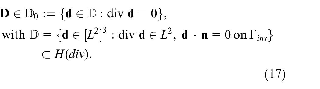
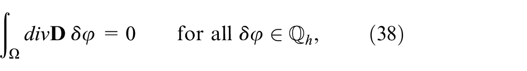
In an electrostatic regime on a simply connected domain, the electric field $\mathbf{E}$ can be shown to be a gradient field due to Faraday’s law. We use standard nomenclature from the literature, introducing the electric potential $\phi$ with $\mathbf{E}=-\nabla \phi$ . The dielectric displacement vector $\mathbf{D}$ satisfies Gauss’ law of zero charge in the material,

$$\mathrm{div}\mathbf{D}=0\mathrm{in}\mathrm{\Omega }.$$

(1)

Last, we use the remanent polarization ${\mathbf{P}}^i$ as an internal variable.

The reversible material response is characterized by the internal energy $\mathrm{\Psi }$ or its density $\psi$ , which shall depend on strain, dielectric displacement as well as remanent polarization vector,

$$\psi (\mathbf{x},t)=\hat{\psi }(\mathbf{S}(\mathbf{x},t),\mathbf{D}(\mathbf{x},t),{\mathbf{P}}^i(\mathbf{x},t)),$$

(2)

$$\mathrm{\Psi }(t)={\int }_{\mathrm{\Omega }}\psi (\mathbf{x},t)d\mathbf{x}.$$

(3)

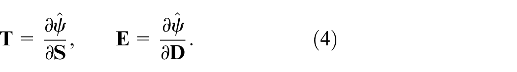
Total stress $\mathbf{T}$ and electric field $\mathbf{E}$ are conjugate to strain $\mathbf{S}$ and dielectric displacement $\mathbf{D}$ in the following sense,

$$\mathbf{T}=\frac{\partial \hat{\psi }}{\partial \mathbf{S}},\mathbf{E}=\frac{\partial \hat{\psi }}{\partial \mathbf{D}}.$$

(4)

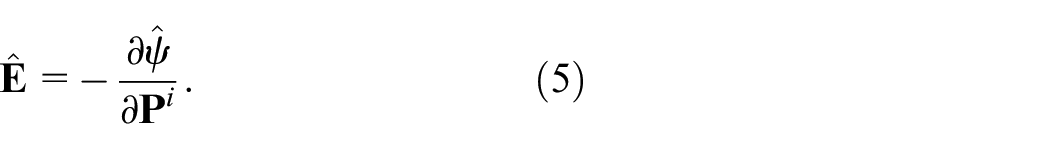
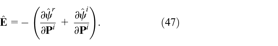
Conjugate to the remanent polarization is the (negative) electric driving force $\hat{\mathbf{E}}$ ,

$$\hat{\mathbf{E}}=-\frac{\partial \hat{\psi }}{\partial {\mathbf{P}}^i}.$$

(5)

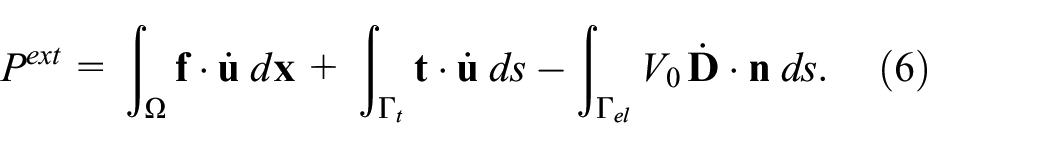
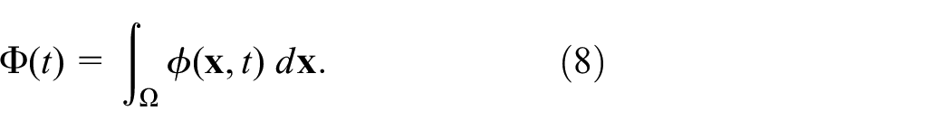
We denote by $P^{\mathrm{ext}}=\frac{d}{\mathrm{dt}}{W}^{\mathrm{ext}}$ the power added from external sources such as applied forces or electric fields. As in mixed methods the external work often differs from standard approaches, we provide an exemplary expression below. For a given volume load $\mathbf{f}$ in $\mathrm{\Omega }$ , a surface load $\mathbf{t}$ on ${\mathrm{\Gamma }}_t$ and an applied electric potential $V_0$ on ${\mathrm{\Gamma }}_{\mathrm{el}}$ , the power from external sources is given by

$$P^{\mathrm{ext}}={\int }_{\mathrm{\Omega }}\mathbf{f}·\stackrel{·}{\mathbf{u}}d\mathbf{x}+{\int }_{{\mathrm{\Gamma }}_t}\mathbf{t}·\stackrel{·}{\mathbf{u}}\mathrm{ds}-{\int }_{{\mathrm{\Gamma }}_{\mathrm{el}}}{V}_0\stackrel{·}{\mathbf{D}}·\mathbf{n}\mathrm{ds}.$$

(6)

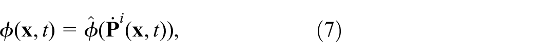
A reversible process is fully characterized by internal energy $\mathrm{\Psi }$ and external work $W^{\mathrm{ext}}$ , and there are no internal variables such as the remanent polarization present. In this contribution however, we are concerned with irreversible, dissipative processes. As stated by Miehe et al. (2011), the dissipative behavior can be described by the dissipation function $\mathrm{\Phi }$ , which depends only on the rate of the internal variable. In our case, the dissipation function is thus a function of the remanent polarization rate,

$$\varphi (\mathbf{x},t)=\hat{\varphi }({\stackrel{·}{\mathbf{P}}}^i(\mathbf{x},t)),$$

(7)

$$\mathrm{\Phi }(t)={\int }_{\mathrm{\Omega }}\varphi (\mathbf{x},t)d\mathbf{x}.$$

(8)

Depending on the dissipation function, rate-dependent or rate-independent material behavior is modeled. In the next section, we motivate our special choice of dissipation function, which leads to rate-independent behavior.

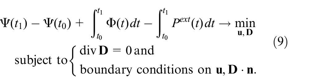
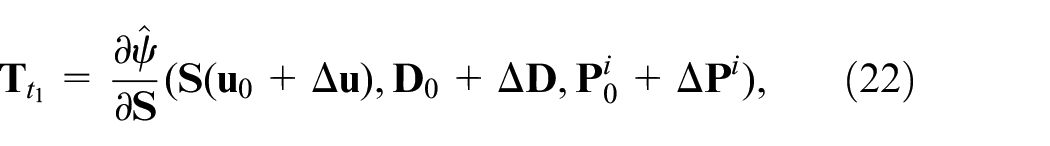
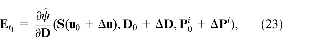
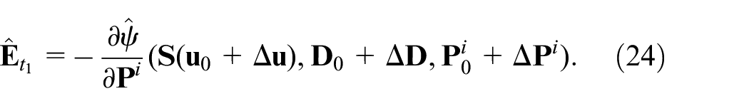
Using the notions introduced above, we cite the following incremental minimization problem for any time interval $(t_0,t_1)$ ,

$$\begin{array}{c}\mathrm{\Psi }(t_1)-\mathrm{\Psi }(t_0)+{\int }_{t_0}^{t_1}\mathrm{\Phi }(t)\mathrm{dt}-{\int }_{t_0}^{t_1}{P}^{\mathrm{ext}}(t)\mathrm{dt}\to \underset{\mathbf{u},\mathbf{D}}{min}\hfill \\ \mathrm{subject}\mathrm{to}\{\begin{array}{c}\mathrm{div}\mathbf{D}=0\mathrm{and}\hfill \\ \multicolumn{1}{c}{\mathrm{boundary}\mathrm{conditions}\mathrm{on}\mathbf{u},\mathbf{D}·\mathbf{n}.}\end{array}\hfill \end{array}$$

(9)

For a more detailed introduction, we refer to the extensive derivations originally provided by Miehe et al. (2011).

2.1. Choice of internal energy

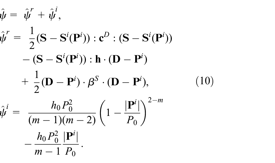
Different choices of the internal energy density have been proposed in the literature. In many contributions, the internal energy is decomposed into two additive terms: the first of these terms coincides with the energy in linear problems for fixed remanent polarization. It is quadratic in the reversible parts of dielectric displacement and strain, but material tensors ${\mathbf{c}}^D,\mathbf{h}$ and ${\beta }^S$ may depend on the remanent polarization. The second term depends then only on the remanent polarization, and contains the electric hysteresis shape parameters $h_0$ and m and the saturation polarization $P_0$ .

$$\begin{array}{c}\hat{\psi }={\hat{\psi }}^r+{\hat{\psi }}^i,\hfill \\ {\hat{\psi }}^r=\frac{1}{2}(\mathbf{S}-{\mathbf{S}}^i({\mathbf{P}}^i)):{\mathbf{c}}^D:(\mathbf{S}-{\mathbf{S}}^i({\mathbf{P}}^i))\hfill \\ -(\mathbf{S}-{\mathbf{S}}^i({\mathbf{P}}^i)):\mathbf{h}·(\mathbf{D}-{\mathbf{P}}^i)\hfill \\ +\frac{1}{2}(\mathbf{D}-{\mathbf{P}}^i)·{\beta }^S·(\mathbf{D}-{\mathbf{P}}^i),\hfill \\ {\hat{\psi }}^i=\frac{h_0{P}_0^2}{(m-1)(m-2)}{(1-\frac{|{\mathbf{P}}^i|}{P_0})}^{2-m}\hfill \\ -\frac{h_0{P}_0^2}{m-1}\frac{|{\mathbf{P}}^i|}{P_0}.\hfill \end{array}$$

(10)

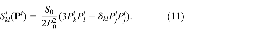
We use a one-to-one relationship between remanent polarization and polarization strain as suggested by McMeeking and Landis (2002),

$$S_{\mathrm{kl}}^i({\mathbf{P}}^i)=\frac{S_0}{2P_0^2}(3P_k^i{P}_l^i-{\delta }_{\mathrm{kl}}{P}_j^i{P}_j^i).$$

(11)

Note that this choice is volume preserving.

2.2. Choice of dissipation function

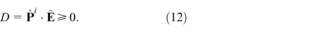
Apart from the free energy density $\hat{\psi }$ , the dissipation function $\hat{\varphi }$ has to be specified to obtain a valid model through the minimization problem (9). The dissipation function is closely related to the dissipation D. The dissipation describes the amount of energy dissipated into heat and is always non-negative, as stated by the Clausius-Duhem inequality

$$D={\stackrel{·}{\mathbf{P}}}^i·\hat{\mathbf{E}}\ge 0.$$

(12)

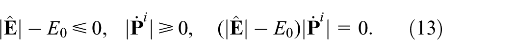
The choice of dissipation function $\hat{\varphi }$ is motivated by the principle of maximum dissipation. It is closely related to the switching condition, which states in its simplest form that the remanent polarization rate is non-trivial only if the driving electric field $\hat{\mathbf{E}}$ exceeds the coercive field $E_0$ ,

$$|\hat{\mathbf{E}}|-E_0\le 0,|{\stackrel{·}{\mathbf{P}}}^i|\ge 0,(|\hat{\mathbf{E}}|-E_0)|{\stackrel{·}{\mathbf{P}}}^i|=0.$$

(13)

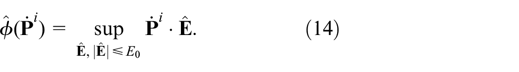
The dissipation function is chosen such that dissipation is maximized over all possible values for $\hat{\mathbf{E}}$ ,

$$\hat{\varphi }({\stackrel{·}{\mathbf{P}}}^i)=\underset{\hat{\mathbf{E}},|\hat{\mathbf{E}}|\le E_0}{sup}{\stackrel{·}{\mathbf{P}}}^i·\hat{\mathbf{E}}.$$

(14)

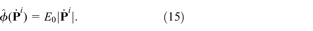
This supremum is of course taken for $\hat{\mathbf{E}}=E_0{\mathbf{e}}_P$ , with ${\mathbf{e}}_P={\mathbf{P}}^i/|{\mathbf{P}}^i|$ the unit vector in direction of remanent polarization, and for $\hat{\mathbf{E}}=0$ in case $|{\stackrel{·}{\mathbf{P}}}^i|=0$ . Thus, the dissipation function can be simplified to read

$$\hat{\varphi }({\stackrel{·}{\mathbf{P}}}^i)=E_0|{\stackrel{·}{\mathbf{P}}}^i|.$$

(15)

Note that this dissipation function is positively homogeneous (compare (20)). Such a dissipation function leads to rate-independent behavior, see Miehe et al. (2011).

3. Mathematical modeling

To get a well-defined problem in a mathematical sense, we introduce Hilbert spaces for the various quantities. Then, the time-discrete minimization problem (9) can be solved minimizing in the respective closed spaces. We use the standard $H^1$ Sobolev space of weakly differentiable functions with derivative in $L^2$ for the displacements. (Homogeneous) displacement boundary conditions on the boundary part ${\mathrm{\Gamma }}_{\mathrm{fix}}$ are included, such that we are searching for

$$\mathbf{u}\in \mathbb{V}:=\{\mathbf{v}\in H^1(\mathrm{\Omega }):\mathbf{v}=0\mathrm{on}{\mathrm{\Gamma }}_{\mathrm{fix}}\}.$$

(16)

The choice of the dielectric displacement space is less standard. We resort to the $H(\mathrm{div})$ space of $L^2$ vector fields with weak divergence. Gauss’ law (1) is then included explicitely. Additionally, insulation boundary conditions of vanishing surface charges $\mathbf{D}·\mathbf{n}=0$ are posed explicitely. This means that these surface charge boundary conditions are essential boundary conditions, while we have already seen in the power statement (6) that voltage boundary conditions on electrodes are natural. Summing up, we search for

$$\begin{array}{c}\mathbf{D}\in {\mathbb{D}}_0:=\{\mathbf{d}\in \mathbb{D}:\mathrm{div}\mathbf{d}=0\},\hfill \\ \mathrm{with}\mathbb{D}=\{\mathbf{d}\in [L^2{]}^3:\mathrm{div}\mathbf{d}\in L^2,\mathbf{d}·\mathbf{n}=0\mathrm{on}{\mathrm{\Gamma }}_{\mathrm{ins}}\}\hfill \\ \subset H(\mathrm{div}).\hfill \end{array}$$

(17)

The remanent polarization does not sport any smoothness, nor does it allow for boundary conditions. Therefore we choose the vector-valued Lebesgue space $[L^2{]}^3$ ,

$${\mathbf{P}}^i\in \mathbb{P}:=[L^2{]}^3.$$

(18)

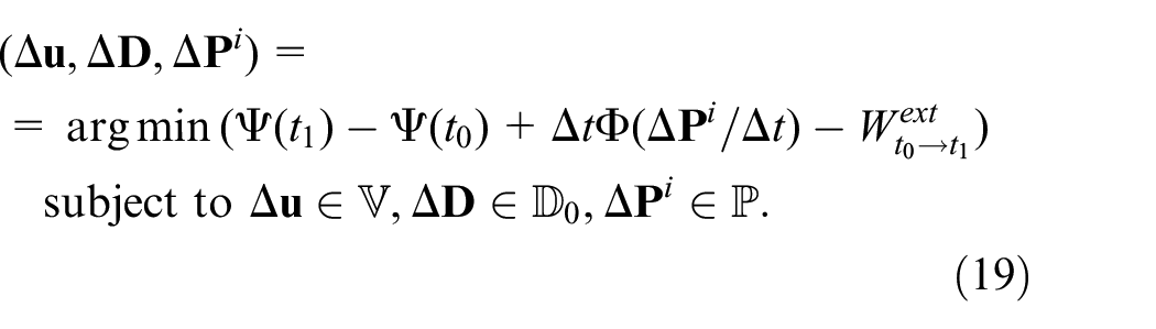
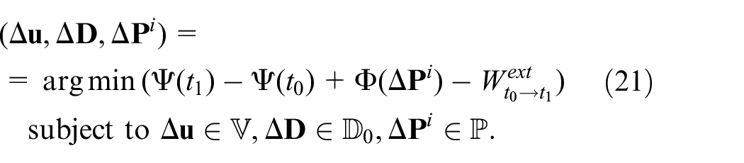
We will now formulate the incremental variational problem for some small but finite time increment $\mathrm{\Delta }t$ , starting from time $t_0$ to $t_1=t_0+\mathrm{\Delta }t$ . To this end, we assume ${\mathbf{u}}_0=\mathbf{u}(t_0)$ , ${\mathbf{D}}_0=\mathbf{D}(t_0)$ and ${\mathbf{P}}_0^i={\mathbf{P}}^i(0)$ known. We are interested in finding the increments $\mathrm{\Delta }\mathbf{u},\mathrm{\Delta }\mathbf{D}$ and $\mathrm{\Delta }{\mathbf{P}}^i$ such that $\mathbf{u}(t_1)={\mathbf{u}}_0+\mathrm{\Delta }\mathbf{u}$ , $\mathbf{D}(t_1)={\mathbf{D}}_0+\mathrm{\Delta }\mathbf{D}$ and ${\mathbf{P}}^i(t_1)={\mathbf{P}}_0^i+\mathrm{\Delta }{\mathbf{P}}^i$ . Miehe et al. (2011) stated that these increments minimize the potential increment,

$$\begin{array}{c}(\mathrm{\Delta }\mathbf{u},\mathrm{\Delta }\mathbf{D},\mathrm{\Delta }{\mathbf{P}}^i)=\hfill \\ =\arg min(\mathrm{\Psi }(t_1)-\mathrm{\Psi }(t_0)+\mathrm{\Delta }t\mathrm{\Phi }(\mathrm{\Delta }{\mathbf{P}}^i/\mathrm{\Delta }t)-W_{t_0\to t_1}^{\mathrm{ext}})\hfill \\ \mathrm{subject}\mathrm{to}\mathrm{\Delta }\mathbf{u}\in \mathbb{V},\mathrm{\Delta }\mathbf{D}\in {\mathbb{D}}_0,\mathrm{\Delta }{\mathbf{P}}^i\in \mathbb{P}.\hfill \end{array}$$

(19)

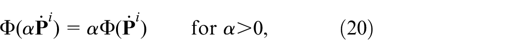
In the special case of a rate-independent response, where the dissipation function is positively homogeneous,

$$\mathrm{\Phi }(\alpha {\stackrel{·}{\mathbf{P}}}^i)=\alpha \mathrm{\Phi }({\stackrel{·}{\mathbf{P}}}^i)\mathrm{for}\alpha >0,$$

(20)

the time step size cancels out in (19). The parameter t acts as pseudo-time then, the minimization problem reads

$$\begin{array}{c}(\mathrm{\Delta }\mathbf{u},\mathrm{\Delta }\mathbf{D},\mathrm{\Delta }{\mathbf{P}}^i)=\hfill \\ =\arg min(\mathrm{\Psi }(t_1)-\mathrm{\Psi }(t_0)+\mathrm{\Phi }(\mathrm{\Delta }{\mathbf{P}}^i)-W_{t_0\to t_1}^{\mathrm{ext}})\hfill \\ \mathrm{subject}\mathrm{to}\mathrm{\Delta }\mathbf{u}\in \mathbb{V},\mathrm{\Delta }\mathbf{D}\in {\mathbb{D}}_0,\mathrm{\Delta }{\mathbf{P}}^i\in \mathbb{P}.\hfill \end{array}$$

(21)

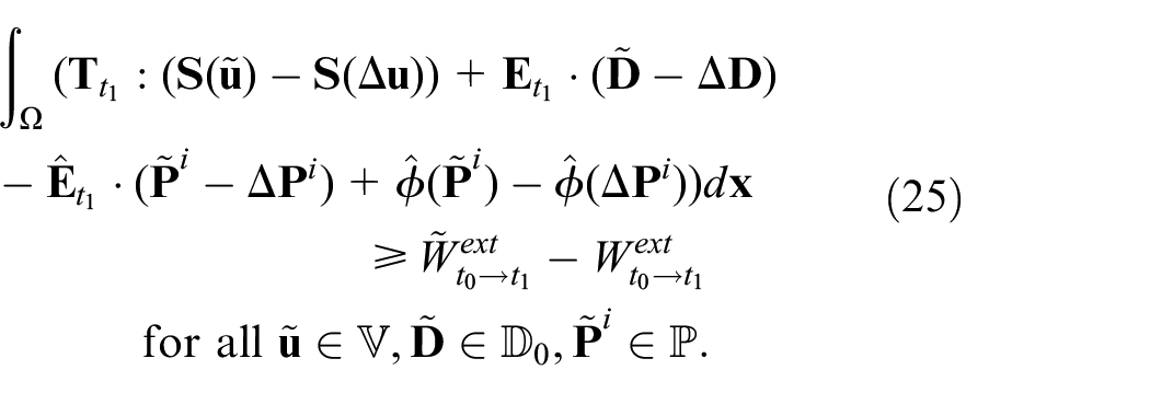
3.1. Variational inequality

As the dissipation function is not differentiable at ${\stackrel{·}{\mathbf{P}}}^i=0$ , this minimization problem cannot be transformed into a variational equation. However, it can be treated in the framework of variational inequalities. Inspired by the mathematical analysis of elasto-plasticity (see e.g. Han and Reddy (1999)) or contact problems (see e.g. Sofonea and Matei (2011)), a thorough analysis of the arising time-dependent variational inequality has been carried out in Pechstein et al. (2020). In this contribution, we state the variational inequality which is equivalent to the optimization problem (21). We use the definitions for total stress $\mathbf{T}$ and electric field $\mathbf{E}$ (4) and for the electric driving force $\hat{\mathbf{E}}$ (5) evaluated at $t_1$ ,

$${\mathbf{T}}_{t_1}=\frac{\partial \hat{\psi }}{\partial \mathbf{S}}(\mathbf{S}({\mathbf{u}}_0+\mathrm{\Delta }\mathbf{u}),{\mathbf{D}}_0+\mathrm{\Delta }\mathbf{D},{\mathbf{P}}_0^i+\mathrm{\Delta }{\mathbf{P}}^i),$$

(22)

$${\mathbf{E}}_{t_1}=\frac{\partial \hat{\psi }}{\partial \mathbf{D}}(\mathbf{S}({\mathbf{u}}_0+\mathrm{\Delta }\mathbf{u}),{\mathbf{D}}_0+\mathrm{\Delta }\mathbf{D},{\mathbf{P}}_0^i+\mathrm{\Delta }{\mathbf{P}}^i),$$

(23)

$${\hat{\mathbf{E}}}_{t_1}=-\frac{\partial \hat{\psi }}{\partial {\mathbf{P}}^i}(\mathbf{S}({\mathbf{u}}_0+\mathrm{\Delta }\mathbf{u}),{\mathbf{D}}_0+\mathrm{\Delta }\mathbf{D},{\mathbf{P}}_0^i+\mathrm{\Delta }{\mathbf{P}}^i).$$

(24)

Then, $\mathrm{\Delta }\mathbf{u}\in \mathbb{V}$ , $\mathrm{\Delta }\mathbf{D}\in {\mathbb{D}}_0$ and $\mathrm{\Delta }{\mathbf{P}}^i\in \mathbb{P}$ satisfy the following variational inequality

$$\begin{array}{c}{\int }_{\mathrm{\Omega }}({\mathbf{T}}_{t_1}:(\mathbf{S}(\tilde{\mathbf{u}})-\mathbf{S}(\mathrm{\Delta }\mathbf{u}))+{\mathbf{E}}_{t_1}·(\tilde{\mathbf{D}}-\mathrm{\Delta }\mathbf{D})\hfill \\ -{\hat{\mathbf{E}}}_{t_1}·({\tilde{\mathbf{P}}}^i-\mathrm{\Delta }{\mathbf{P}}^i)+\hat{\varphi }({\tilde{\mathbf{P}}}^i)-\hat{\varphi }(\mathrm{\Delta }{\mathbf{P}}^i))d\mathbf{x}\hfill \\ \ge {\tilde{W}}_{t_0\to t_1}^{\mathrm{ext}}-W_{t_0\to t_1}^{\mathrm{ext}}\hfill \\ \mathrm{for}\mathrm{all}\tilde{\mathbf{u}}\in \mathbb{V},\tilde{\mathbf{D}}\in {\mathbb{D}}_0,{\tilde{\mathbf{P}}}^i\in \mathbb{P}.\hfill \end{array}$$

(25)

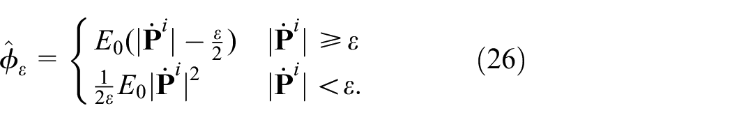
3.2. Regularization

In the framework of elasto-plasticity, Han and Reddy (1999) propose to regularize the dissipation function. The dissipation function is changed slightly, such that it becomes differentiable everywhere. When using the regularized dissipation function, the variational inequality (25) turns into a nonlinear variational equation, which can be solved by standard nonlinear solution algorithms.

We propose to use the regularized dissipation function

$${\hat{\varphi }}_{\epsilon }=\{\begin{array}{cc}{E}_0(|{\stackrel{·}{\mathbf{P}}}^i|-\frac{\epsilon }{2})\hfill & |{\stackrel{·}{\mathbf{P}}}^i|\ge \epsilon \hfill \\ \multicolumn{1}{c}{\frac{1}{2\epsilon }{E}_0|{\stackrel{·}{\mathbf{P}}}^i{|}^2}& |{\stackrel{·}{\mathbf{P}}}^i|<\epsilon .\hfill \end{array}$$

(26)

This choice has been analyzed to work well for elasto-plasticity in Han and Reddy (1999). Indeed, according to this reference, we expect the error due to regularization to be of order $\sqrt{\epsilon }$ .

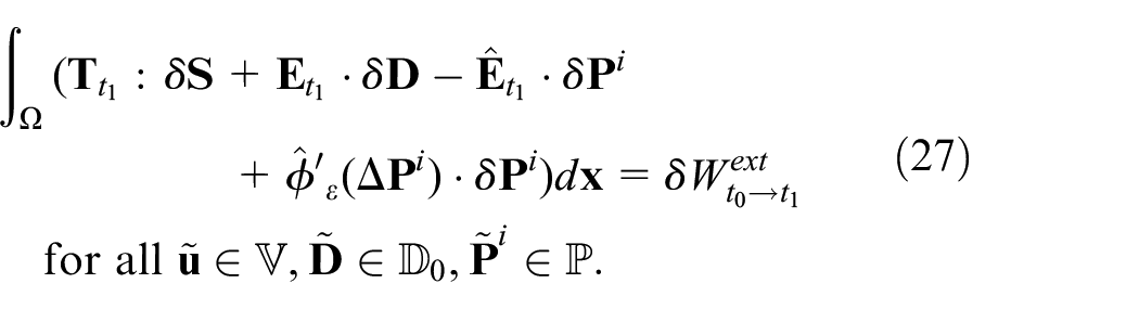
For completeness we provide the variational equation to be solved in each time step. We denote the (continuous) derivative of the regularized dissipation function ${\hat{\varphi }}_{\epsilon }$ with respect to the remanent polarization rate as $\hat{\varphi }{\prime }_{\epsilon }$ . The updates $\mathrm{\Delta }\mathbf{u}\in \mathbb{V}$ , $\mathrm{\Delta }\mathbf{D}\in {\mathbb{D}}_0$ and $\mathrm{\Delta }{\mathbf{P}}^i\in \mathbb{P}$ satisfy

$$\begin{array}{c}{\int }_{\mathrm{\Omega }}({\mathbf{T}}_{t_1}:\delta \mathbf{S}+{\mathbf{E}}_{t_1}·\delta \mathbf{D}-{\hat{\mathbf{E}}}_{t_1}·\delta {\mathbf{P}}^i\hfill \\ +{\hat{\varphi }\prime }_{\epsilon }(\mathrm{\Delta }{\mathbf{P}}^i)·\delta {\mathbf{P}}^i)d\mathbf{x}=\delta W_{t_0\to t_1}^{\mathrm{ext}}\hfill \\ \mathrm{for}\mathrm{all}\tilde{\mathbf{u}}\in \mathbb{V},\tilde{\mathbf{D}}\in {\mathbb{D}}_0,{\tilde{\mathbf{P}}}^i\in \mathbb{P}.\hfill \end{array}$$

(27)

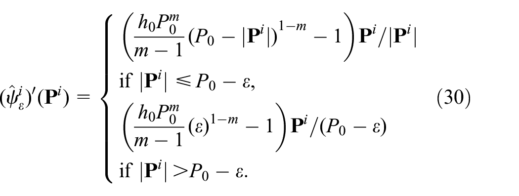
Another issue for regularization is the free energy function $\psi$ , or its additive part ${\psi }^i$ . The formula proposed in (10) is unbounded as the saturation polarization is approached,

$${\hat{\psi }}^i({\mathbf{P}}^i)\to \infty \mathrm{and}({\hat{\psi }}^i)\prime ({\mathbf{P}}^i)·\delta {\mathbf{P}}^i\to \infty$$

(28)

$$\mathrm{as}|{\mathbf{P}}^i|\to P_0.$$

(29)

This unbounded potential acts as a penalty term as the polarization approaches saturation, where also $({\hat{\psi }}^i)\prime ({\mathbf{P}}^i)$ diverges to infinity. As analyzed in Pechstein et al. (2020), this fact does not harm solvability of the update equation (27) itself, but it may harm convergence. Therefore, if convergence problems are observed, we propose to modify the energy density ${\hat{\psi }}^i$ in a way that $({\hat{\psi }}_{\epsilon }^i)\prime ({\mathbf{P}}^i)$ becomes large but stays bounded. We use the following regularized expression $({\hat{\psi }}_{\epsilon }^i)\prime$ ,

$$({\hat{\psi }}_{\epsilon }^i)\prime ({\mathbf{P}}^i)=\{\begin{array}{c}(\frac{h_0{P}_0^m}{m-1}{(P_0-|{\mathbf{P}}^i|)}^{1-m}-1){\mathbf{P}}^i/|{\mathbf{P}}^i|\hfill \\ \mathrm{if}|{\mathbf{P}}^i|\le P_0-\epsilon ,\hfill \\ (\frac{h_0{P}_0^m}{m-1}{(\epsilon )}^{1-m}-1){\mathbf{P}}^i/(P_0-\epsilon )\hfill \\ \mathrm{if}|{\mathbf{P}}^i|>P_0-\epsilon .\hfill \end{array}$$

(30)

3.3. Gauss’ law

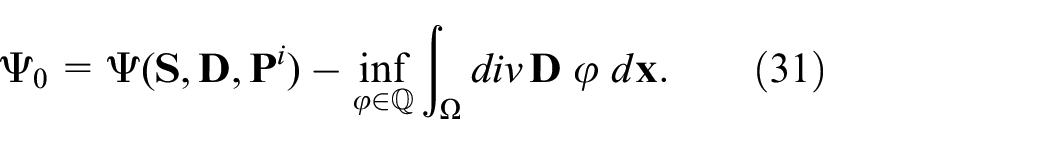
Gauss’ law of zero charges (1) implies that the dielectric displacement field is divergence free inside the domain $\mathrm{\Omega }$ . So far, this condition has been included in the space of admissible updates ${\mathbb{D}}_0$ without further ceremony. As Gauss’ law is a linear and continuous restriction, the space ${\mathbb{D}}_0$ is a linear and continuous subspace of $\mathbb{D}$ and $H(\mathrm{div})$ . However, as this condition is non-local, it will be difficult to implement a finite element space consisting of divergence-free finite element functions in practice. In the following paragraph, we discuss how to reformulate the condition in an equivalent way, such that finite element implementation will be possible. We stress that, both in theory in this section, as well as in the finite element implementation, the dielectric displacement field will be exactly divergence free in the strong sense.

We propose to add a Lagrangian multiplier ensuring the divergence-free condition. As it turns out that this multiplier resembles the electric potential, we denominate it as $\phi$ . In the minimization problem, we propose to use an augmented energy ${\mathrm{\Psi }}_0$ , which assumes infinity if Gauss’ law is violated. This augmented energy reads

$${\mathrm{\Psi }}_0=\mathrm{\Psi }(\mathbf{S},\mathbf{D},{\mathbf{P}}^i)-\underset{\phi \in \mathbb{Q}}{inf}{\int }_{\mathrm{\Omega }}\mathrm{div}\mathbf{D}\phi d\mathbf{x}.$$

(31)

Note that we use $\phi \in \mathbb{Q}:=L^2(\mathrm{\Omega })$ , which means that discontinuous electric potentials are admissible testing functions. Also, the electric potential does not satisfy any boundary conditions a priori. Of course, as the approach is consistent, the potential will assume boundary values matching the prescribed external work (6). Also, it is not necessary to implement an equi-potential condition on electrodes specifically.

The regularized variational equation including Gauss’ law is stated below. The updates $\mathrm{\Delta }\mathbf{u}\in \mathbb{V}$ , $\mathrm{\Delta }\mathbf{D}\in \mathbb{D}$ and $\mathrm{\Delta }{\mathbf{P}}^i\in \mathbb{P}$ as well as the (total) electric potential $\phi \in \mathbb{Q}$ satisfy

$$\begin{array}{c}{\int }_{\mathrm{\Omega }}({\mathbf{T}}_{t_1}:\delta \mathbf{S}+{\mathbf{E}}_{t_1}·\delta \mathbf{D}-{\hat{\mathbf{E}}}_{t_1}·\delta {\mathbf{P}}^i\hfill \\ -\mathrm{div}(\delta \mathbf{D})\phi -\mathrm{div}(\mathrm{\Delta }\mathbf{D})\delta \phi \hfill \\ +{\hat{\varphi }\prime }_{\epsilon }(\mathrm{\Delta }{\mathbf{P}}^i)·\delta {\mathbf{P}}^i)d\mathbf{x}=\delta W_{t_0\to t_1}^{\mathrm{ext}}\hfill \\ \mathrm{for}\mathrm{all}\delta \mathbf{u}\in \mathbb{V},\delta \mathbf{D}\in \mathbb{D},\delta {\mathbf{P}}^i\in \mathbb{P},\delta \phi \in \mathbb{Q}.\hfill \end{array}$$

(32)

The augmented variational equation (32) is equivalent to (27). The dielectric displacement update $\mathrm{\Delta }\mathbf{D}$ is exactly divergence free and thus $\mathrm{\Delta }\mathbf{D}\in {\mathbb{D}}_0$ .

3.4. Solvability and stability

The issue of existence of solutions, also to the time-dependent variational inequality (25), has been treated by the authors in Pechstein et al. (2020). We recall that a unique solution to the update problem (25) exists, given the following essential assumption of strong monotonicity holds: for all $\mathbf{u},\tilde{\mathbf{u}}\in \mathbb{V}$ , $\mathbf{D},\tilde{\mathbf{D}}\in {\mathbb{D}}_0$ and ${\mathbf{P}}^i,{\tilde{\mathbf{P}}}^i\in \mathbb{P}$ as well as corresponding forces $\mathbf{T},\tilde{\mathbf{T}}$ , $\mathbf{E},\tilde{\mathbf{E}}$ and $\hat{\mathbf{E}},\widetilde{\hat{\mathbf{E}}}$ there holds

$$\begin{array}{c}{\int }_{\mathrm{\Omega }}((\mathbf{T}-\tilde{\mathbf{T}}):(\mathbf{S}-\tilde{\mathbf{S}})+(\mathbf{E}-\tilde{\mathbf{E}})·(\mathbf{D}-\tilde{\mathbf{D}})\hfill \\ -(\hat{\mathbf{E}}-\widetilde{\hat{\mathbf{E}}})·({\mathbf{P}}^i-{\tilde{\mathbf{P}}}^i))d\mathbf{x}\hfill \\ \ge C(\parallel \mathbf{u}-\tilde{\mathbf{u}}{\parallel }_{\mathbb{V}}^2+\parallel \mathbf{D}-\tilde{\mathbf{D}}{\parallel }_{\mathbb{D}}^2+\parallel {\mathbf{P}}^i-{\tilde{\mathbf{P}}}^i{\parallel }_{\mathbb{P}}^2).\hfill \end{array}$$

(33)

This is the case if the reversible part of energy ${\mathrm{\Psi }}^r$ is strongly monotone with respect to the reversible parts $\mathbf{S}-{\mathbf{S}}^i({\mathbf{P}}^i)$ and $\mathbf{D}-{\mathbf{P}}^i$ , and the additive part ${\mathrm{\Psi }}^i$ is strongly monotone with respect to ${\mathbf{P}}^i$ . This is the case, as long as the linear moduli lead to a positive definite material tensor. This issue is addressed by Stark et al. (2016c). Conditions ensuring positive definiteness of the additive energy part ${\hat{\psi }}^i$ can be found in Bottero and Idiart (2018).

4. Finite elements

In this section we propose a set of consistent finite elements to discretize the variational equation (32) above. The elements shall be of arbitrary order, by $k\ge 1$ we denote the lowest overall polynomial order. In the following, we assume that $\mathcal{T}$ is a simplicial mesh of the volume $\mathrm{\Omega }$ . The elements can be defined also on prismatic meshes, as is shown in our numerical results. Note that, in the context of our mixed elements, consistent does not necessarily mean continuous— while consistent displacement elements are indeed continuous, consistent elements for the dielectric displacement have a continuous normal component, and elements for the electric potential and remanent polarization are fully discontinuous.

4.1. Displacement elements

The displacement element has to be consistent for $H^1$ , such that $\mathbf{u}\in \mathbb{V}$ . This condition is satisfied when using standard nodal or hierarchical continuous elements. We propose to use hierarchical elements of arbitrary order. For simplicial elements, the finite element space ${\mathbb{V}}_h$ is then given by

$${\mathbb{V}}_h:=\{\mathbf{v}\in \mathcal{C}(\mathrm{\Omega }):\mathbf{v}{|}_T\in [P^{k+1}{]}^3\mathrm{for}T\in \mathcal{T}\}\subset \mathbb{V}.$$

(34)

For tetrahedral elements, this results in $(k+2)(k+3)(k+4)/2$ degrees of freedom, which means $30$ degrees of freedom for $k=1$ (second order displacment elements) and $60$ degrees of freedom for $k=2$ (third order displacment element). A prismatic element sports $3(k+2{)}^2(k+3)/2$ degrees of freedom. For $k=1$ this results in $54$ degrees of freedom (second order displacment elements), for $k=2$ we obtain $120$ degrees of freedom (third order displacment elements).

4.2. Dielectric displacement and electric potential

The dielectric displacement elements are less standard. To be consistent, we need that $\mathbf{D}\in \mathbb{D}$ , i.e. that $\mathbf{D}$ allows for a divergence in weak sense. This means that the elements need to be normal continuous. In other words, different moments of the normal component $\mathbf{D}·\mathbf{n}$ on element interfaces are degrees of freedom instead of nodal values. Different families of such normal-continuous elements have been introduced in the literature. For a fundamental introduction and overview, we refer the interested reader to the monograph Boffi et al. (2013). As a first proposition, we propose to use elements from the BDM family as introduced by Brezzi et al. (1987) (BDM after Brezzi, Douglas and Marini, who first proposed corresponding elements in two dimensions, see Brezzi et al. (1986)). These elements span the space

$$\begin{array}{c}{\mathbb{D}}_h:=\{\mathbf{D}\in [L^2(\mathrm{\Omega }){]}^3:\mathbf{D}{|}_T\in [P^k{]}^3\mathrm{for}T\in \mathcal{T},\hfill \\ \mathbf{D}·\mathbf{n}\mathrm{cont}.,\mathbf{D}·\mathbf{n}=0\mathrm{on}{\mathrm{\Gamma }}_{\mathrm{ins}}\}\subset \mathbb{D}.\hfill \end{array}$$

(35)

However, as the dielectric displacement is divergence free, the number of unknowns can be further reduced. As already mentioned, the divergence-free condition is non-local, therefore it is not possible to restrict the space ${\mathbb{D}}_h$ such that it becomes a subspace of ${\mathbb{D}}_0$ in a simple, local manner. However, in context of incompressible Navier-Stokes equation, Lehrenfeld and Schöberl (2016) have shown that it is possible to do so for the higher-order shape functions. We propose to use this reduced set,

$$\begin{array}{c}{\mathbb{D}}_{h0}:=\{\mathbf{D}\in [L^2(\mathrm{\Omega }){]}^3:\mathbf{D}{|}_T\in [P^k{]}^3\mathrm{for}T\in \mathcal{T},\hfill \\ \mathrm{div}\mathbf{D}{|}_T\in P^0\mathrm{for}T\in \mathcal{T},\hfill \\ \mathbf{D}·\mathbf{n}\mathrm{cont}.,\mathbf{D}·\mathbf{n}=0\mathrm{on}{\mathrm{\Gamma }}_{\mathrm{ins}}\}\subset \mathbb{D}.\hfill \end{array}$$

(36)

We see that this way not only the number of unknowns for $\mathbf{D}$ drops, but also less Lagrangian multipliers $\phi$ are needed. As $\mathrm{div}\mathbf{D}$ is constant per element, it is enough to use piecewise constant $\phi$ ,

$${\mathbb{Q}}_h:=\{\phi \in L^2(\mathrm{\Omega }):\phi {|}_T\in P^0\mathrm{for}T\in \mathcal{T}\}$$

(37)

Then, the condition

$${\int }_{\mathrm{\Omega }}\mathrm{div}\mathbf{D}\delta \phi =0\mathrm{for}\mathrm{all}\delta \phi \in {\mathbb{Q}}_h,$$

(38)

implies that $\mathrm{div}\mathbf{D}=0$ in strong sense for $\mathbf{D}\in {\mathbb{D}}_{h0}$ .

The finite element space ${\mathbb{D}}_{h0}$ is intrinsically different from standard nodal finite element spaces well-known in mechanics. While in nodal finite element spaces such as ${\mathbb{V}}_h$ degrees of freedom are function values evaluated at element nodes, a more abstract concept of degrees of freedom as introduced by Ciarlet (1978) is needed in the context of $H(\mathrm{div})$ . In our case, degrees of freedom are associated to element interfaces (to $\mathbf{D}·\mathbf{n}$ ), and additional “element bubbles” that are associated to the element interior (similar to element-interior nodes). There are no degrees of freedom associated to nodes or element edges. Different from standard nodal elements as used for the displacements, the inter-element coupling acts only through degrees of freedom associated to element faces. Therefore, the coupling is less strong than for standard elements, and even for the same number of overall degrees of freedom, the system matrix is sparser and thereby easier to invert by a direct solver. As the system matrix is indefinite, it is important to choose a direct solver that can handle such systems.

We count the total number of degrees of freedom for the electric quantities per element. In all cases, one degree of freedom is used for the electric potential, while the number of dielectric displacement degrees of freedom varies depending on k and the element shape. For a tetrahedral element of order k, there are $2(k+1)(k+2)$ coupling and $k(k-1)(2k+5)/6$ interior degrees of freedom. For $k=1$ this means $12$ coupling degrees of freedom only, for $k=2$ this adds up to $24$ coupling and $3$ interior degrees of freedom. For a prismatic element, we have $(k+1)(k+2)+3(k+1{)}^2$ coupling and $(k+2)(k+1)(2k+1)/2+1$ interior degrees of freedom. For a first order element with $k=1$ this adds up to $18$ coupling and $10$ inner degrees of freedom. For a second order element with $k=2$ we get $39$ coupling and $31$ inner degrees of freedom.

4.3. Remanent polarization

There are no conditions on the remanent polarization other than ${\mathbf{P}}^i\in \mathbb{P}=[L^2{]}^3$ . Neither in derivation nor in stability analysis any assumptions on the continuity of ${\mathbf{P}}^i$ were made. Therefore, we propose the remanent polarization to be of the same order as the dielectric displacement and discontinuous,

$${\mathbb{P}}_h:=\{{\mathbf{P}}^i\in [L^2(\mathrm{\Omega }){]}^3:{\mathbf{P}}^i{|}_T\in [P^k{]}^3\mathrm{for}T\in \mathcal{T}\}$$

(39)

4.4. Implementation

All finite elements described in this section are implemented in the open source software package Netgen/NGSolve available from ngsolve.org. Netgen/NGSolve sports a python interface, where one can symbolically enter variational equations or energies. The necessary derivations for iterative methods such as Newton’s iteration are then performed automatically. As all finite elements, including the divergence-conforming ones, are predefined in this software package. The variational equation (32), or the minimization problem corresponding to (21) are entered symbolically, using the definitions (10) for the stored energy and (26) for the regularized dissipation function ${\hat{\varphi }}_{\epsilon }$ .

In the proposed Newton iteration scheme, all terms from (32) need to be evaluated to compute the residual vector. Moreover, to obtain the tangent stiffness matrix in each iterative step, derivatives of the terms in (32) are needed. To ensure reproducability of the method, we shortly comment on the necessary computations. We stress that, in our implementation in Netgen/NGSolve, the derivations were not done by hand, but using automatic differentiation of the corresponding energy terms from (21).

Using the internal energy $\hat{\psi }$ from (10), remanent polarization strain ${\mathbf{S}}^i({\mathbf{P}}^i)$ from (11) and the regularized dissipation function ${\hat{\varphi }}_{\epsilon }$ from (26), we obtain the following formulae for stress and electric field

$$\mathbf{T}={\mathbf{c}}^D({\mathbf{P}}^i):(\mathbf{S}-{\mathbf{S}}^i({\mathbf{P}}^i))-\mathbf{h}({\mathbf{P}}^i{)}^{\mathrm{T}}·(\mathbf{D}-{\mathbf{P}}^i),$$

(40)

$$\mathbf{E}=-\mathbf{h}({\mathbf{P}}^i):(\mathbf{S}-{\mathbf{S}}^i({\mathbf{P}}^i))+{\beta }^S({\mathbf{P}}^i)·(\mathbf{D}-{\mathbf{P}}^i).$$

(41)

If one assumes the stiffness at constant electric field ${\mathbf{c}}^E$ , its inverse ${\mathbf{s}}^E=({\mathbf{c}}^E{)}^{-1}$ and the permittivity at constant stress ${\mathbf{e}}^T$ and its inverse ${\beta }^T=({\epsilon }^T{)}^{-1}$ to be constant and isotropic, and the piezoelectric tensor $\mathbf{d}({\mathbf{P}}^i)$ to depend on the remanent polarization as described by Landis (2002), the material tensors above are given by

$${\mathbf{s}}^D({\mathbf{P}}^i)={\mathbf{s}}^E-\mathbf{d}({\mathbf{P}}^i{)}^{\mathrm{T}}·{\beta }^T·\mathbf{d}({\mathbf{P}}^i),$$

(42)

$${\epsilon }^S={\epsilon }^T-\mathbf{d}({\mathbf{P}}^i):{\mathbf{c}}^E:\mathbf{d}({\mathbf{P}}^i{)}^{\mathrm{T}},$$

(43)

$${\mathbf{c}}^D({\mathbf{P}}^i)=({\mathbf{s}}^D{)}^{-1},$$

(44)

$${\beta }^S({\mathbf{P}}^i)=({\epsilon }^S{)}^{-1},$$

(45)

$$\mathbf{h}({\mathbf{P}}^i)={\beta }^S({\mathbf{P}}^i)·\mathbf{d}({\mathbf{P}}^i):{\mathbf{c}}^E.$$

(46)

Derivatives of $\mathbf{d}$ with respect to ${\mathbf{P}}^i$ are detailed by Landis (2002); using the product rule, and the fact that the derivative of the inverse of a tensor is given by $({\mathbf{A}}^{-1})\prime =-{\mathbf{A}}^{-1}·\mathbf{A}\prime ·{\mathbf{A}}^{-1}$ , derivatives of the material moduli (42)–(46) are straightforward but tedious. In our computations, automatic differentiation was used to ensure the correct computation of all derivatives. These derivatives are needed for the Newton matrix, but also for the computation of the driving force $\hat{\mathbf{E}}$ ,

$$\hat{\mathbf{E}}=-(\frac{\partial {\hat{\psi }}^r}{\partial {\mathbf{P}}^i}+\frac{\partial {\hat{\psi }}^i}{\partial {\mathbf{P}}^i}).$$

(47)

In component notation, the respective terms above evaluate to

$$-\frac{\partial {\hat{\psi }}^r}{P_j^i}=T_{\mathrm{kl}}:\frac{\partial S_{\mathrm{kl}}^i}{\partial P_j^i}+E_j$$

(48)

$$-\frac{1}{2}(S_{\mathrm{kl}}-S_{\mathrm{kl}}^i)\frac{\partial c_{\mathrm{klmn}}^D}{\partial P_j^i}(S_{\mathrm{mn}}-S_{\mathrm{mn}}^i)$$

(49)

$$+(S_{\mathrm{kl}}-S_{\mathrm{kl}}^i)\frac{\partial h_{\mathrm{klm}}}{\partial P_j^i}(D_m-P_m^i)$$

(50)

$$-\frac{1}{2}(D_k-P_k^i)\frac{\partial {\beta }_{\mathrm{kl}}^S}{\partial P_j^i}(D_l-P_l^i),$$

(51)

$$-\frac{\partial {\hat{\psi }}^i}{P_j^i}=-({\hat{\psi }}^i)\prime (|{\mathbf{P}}^i|)\frac{P_j^i}{|{\mathbf{P}}^i|}.$$

(52)

For common choices of ${\hat{\psi }}^i$ such as (10), the limit of $-\partial {\hat{\psi }}^i/P_j^i$ for $|{\mathbf{P}}^i|\to 0$ is well-defined as zero in (52). The divergence $\mathrm{div}\mathbf{D}$ is straightforward for divergence-conforming elements as used for the dielectric displacement. When using the regularized dissipation function ${\hat{\varphi }}_{\epsilon }$ from (26), also its derivative $\hat{\varphi }{\prime }_{\epsilon }$ is well-defined as

$$\hat{\varphi }{\prime }_{\epsilon }(\mathrm{\Delta }{\mathbf{P}}^i)=\{\begin{array}{cc}{E}_0\mathrm{\Delta }{\mathbf{P}}^i/|\mathrm{\Delta }{\mathbf{P}}^i|\hfill & |\mathrm{\Delta }{\mathbf{P}}^i|\ge \epsilon ,\hfill \\ \multicolumn{1}{c}{E_0\mathrm{\Delta }{\mathbf{P}}^i/\epsilon }& |\mathrm{\Delta }{\mathbf{P}}^i|<\epsilon .\hfill \end{array}$$

(53)

With these details, the residual vector can be evaluated according to (32). For the correct implementation of Newton’s method, the system matrix at each iterative step is obtained by deriving the residual by the degrees of freedom. Again, this task is straightforward, but even more tedious than for the residual itself.

In computations, we have seen that neither the computed solution nor the iteration counts change if the following simplification is made: instead of considering ${\beta }^S({\mathbf{P}}^i)$ , we used ${\beta }^S({\mathbf{P}}_{t_{n-1}}^i)$ constant evaluated at the last converged time step. This greatly reduces computational costs, and simplifies the necessary derivations.

5. Numerical results

5.1. Non-proportional loading

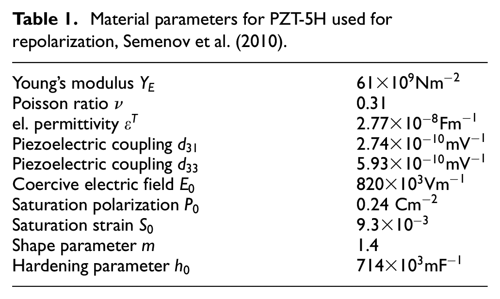
As a first numerical example, we consider the repolarization of a piezoelectric cube. This benchmark problem was originally proposed by Huber and Fleck (2001), who provide measurement results. In their experiment, a cube was cut from pre-polarized PZT-5H, such that the axes of the cube are at an angle $\theta$ compared to the original polarization direction. Then, the cube is electroded and re-polarized by applying an electric field aligned with the cube’s z axis. The change in dielectric displacement at the electrodes was measured with growing prescribed electric field.

This example has been widely used as a benchmark example for non-proportional loading e.g. by McMeeking and Landis (2002); Landis (2002); Arockiarajan et al. (2009); Stark et al. (2016b). In our computations, we assume the cube to be of size $5\mathrm{mm}$ . We use the material parameters for PZT-5H as provided by Semenov et al. (2010), see Table 1, where the $d_{15}$ -effect is neglected. The material is pre-polarized at angle $\theta \in [0^{°},{180}^{°}]$ . The regularization parameter for the dissipation function was chosen as $\epsilon ={10}^{-4}{P}_0$ . The free energy function was not regularized.

Table 1.

Material parameters for PZT-5H used for repolarization, Semenov et al. (2010).

Young’s modulus $Y_E$	$61\times {10}^9{\mathrm{Nm}}^{-2}$
Poisson ratio $\nu$	0.31
el. permittivity ${\epsilon }^T$	$2.77\times {10}^{-8}{\mathrm{Fm}}^{-1}$
Piezoelectric coupling $d_{31}$	$2.74\times {10}^{-10}{\mathrm{mV}}^{-1}$
Piezoelectric coupling $d_{33}$	$5.93\times {10}^{-10}{\mathrm{mV}}^{-1}$
Coercive electric field $E_0$	$820\times {10}^3{\mathrm{Vm}}^{-1}$
Saturation polarization $P_0$	$0.24{\mathrm{Cm}}^{-2}$
Saturation strain $S_0$	$9.3\times {10}^{-3}$
Shape parameter m	1.4
Hardening parameter $h_0$	$714\times {10}^3{\mathrm{mF}}^{-1}$

Concerning this initial state, Stark et al. (2016b) point out that it is not consistent if $\theta \ne 0^{°},{180}^{°}$ , as then surface charges of size ${\rho }_P={\mathbf{P}}^i·\mathbf{n}$ occur at the non-electroded boundaries. In this work, we assume one of their remedy proposals, where these charges are modeled as non-moveable surface charges. This way, on the non-electroded boundaries we have constant surface charges of $\mathbf{D}·\mathbf{n}={\rho }_P$ . For polarization angles $\theta \ne 0^{°},{180}^{°}$ , these boundary conditions lead to a non-homogeneous distribution of the dielectric displacement, with singularities along the electrode boundaries. Therefore, a reasonably fine finite element discretization is necessary. Additionally, finding the equilibrium distribution of $\mathbf{D}$ at zero voltage makes an initial non-linear computation necessary.

In a first computation, we perform repolarization in 20 load steps, where a total electric field of $2E_0$ is applied. We discretize the cube using an unstructured tetrahedral mesh consisting of 745 elements. We choose the finite element order $k=1$ , which means second order displacement elements and first order dielectric/remanent polarization elements. In total, we arrive at eighteen thousand seven hundred thirty three degrees of freedom. In Figure 1 the change in dielectric displacements as measured from the finite element model is provided, together with the original data as taken from Huber and Fleck (2001). A good qualitative resemblance is observed.

Figure 1.

Repoling of piezoelectric cube: The change of dielectric displacement is measured with growing applied electric field for different angles $\theta$ . Comparison to the original measurement data taken from Huber and Fleck (2001).

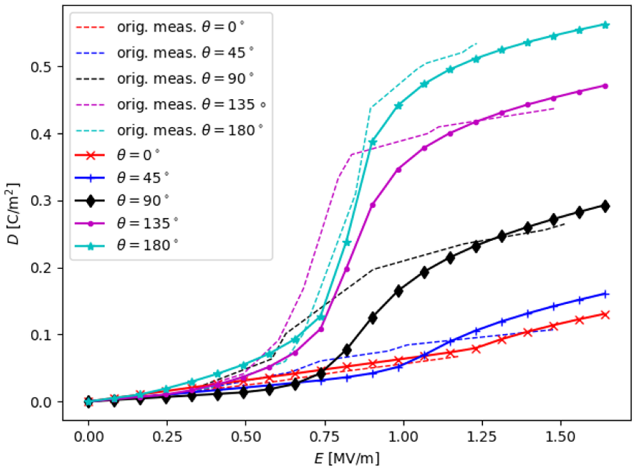
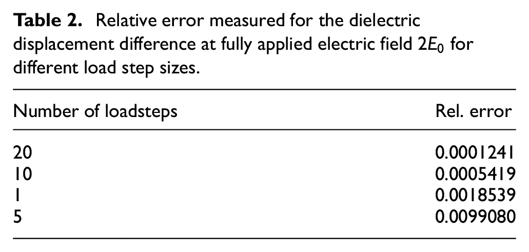
In a second computation, we analyze how the loadstep size affects the results. We consider now the case of $\theta ={90}^{°}$ . We observe that even large load increments lead to accurate results, see Figure 2. In Table 2, the relative error of the dielectric displacement difference measured at an applied electric field of $2E_0$ is provided for different numbers of load steps. To this end, the result from applying 40 loadsteps was used as a reference. We see that using only one load step in this highly nonlinear problem led to a relative error below one percent. In this case, a total number of 35 Newton iterations with line search were needed.

Figure 2.

Repoling of piezoelectric cube: comparison of different loadstep sizes for an initial polarization angle of ${90}^{°}$ .

Table 2.

Relative error measured for the dielectric displacement difference at fully applied electric field $2E_0$ for different load step sizes.

Number of loadsteps	Rel. error
20	0.0001241
10	0.0005419
1	0.0018539
5	0.0099080

5.2. Hexahedron with cylindrical hole

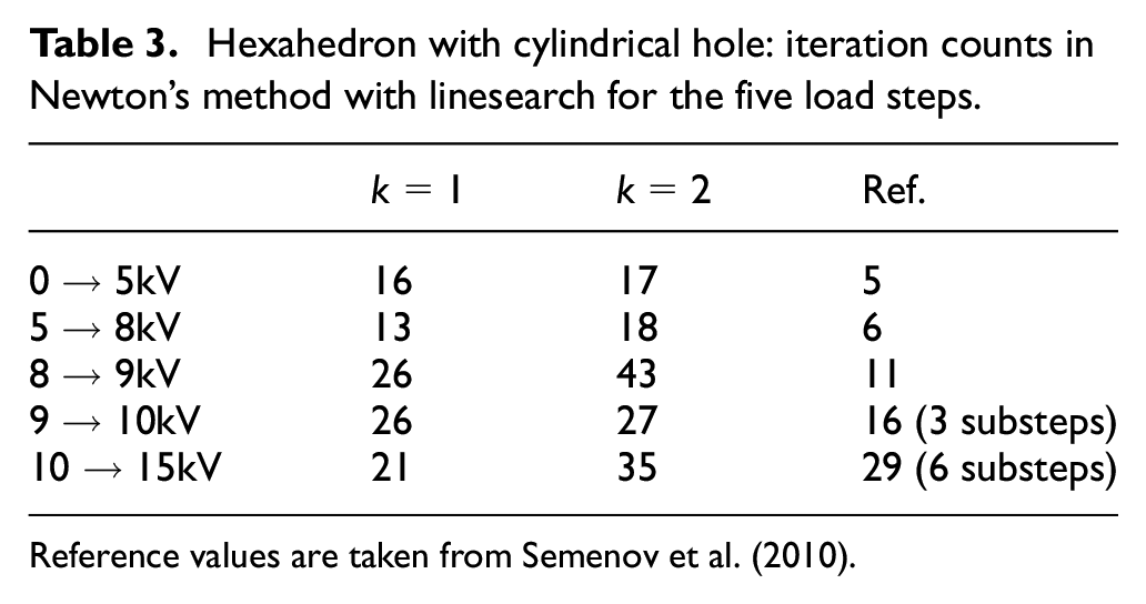
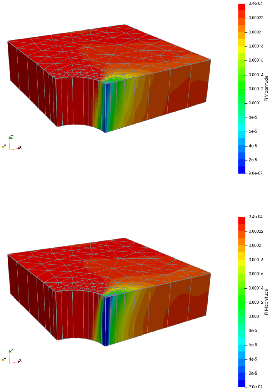
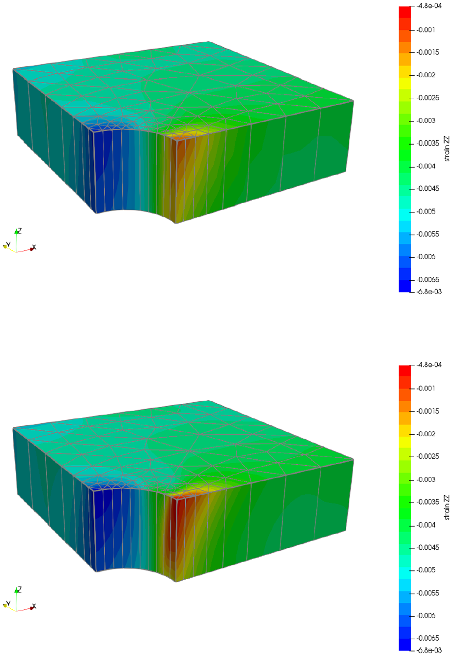
This example is a benchmark example taken from Semenov et al. (2010). A hexahedron of size $l\times l\times h=20\mathrm{mm}\times 20\mathrm{mm}\times 6\mathrm{mm}$ made of PZT-5H sports a cylindrical hole of diameter $r=4\mathrm{mm}$ at the center, $x=y=0$ . Two opposite faces of the hexahedron at $x=\pm l/2$ are electroded, and an electric potential is applied. Stress-free conditions are assumed on the whole boundary. The hexahedron with hole is an interesting benchmark example, as it sports singularities along the curved boundary: at $x=0,y=r$ , high electric fields are expected, leading to quick polarization and (relatively) large deformations in this area, while low electric fields are expected at $y=0,x=r$ , where $D_x=0$ due to the boundary condition. Accordingly, low remanent polarization is expected there even for high applied voltages. Material properties are the same as in the previous example and collected in Table 1. The regularization parameter for the dissipation function was chosen as $\epsilon ={10}^{-4}{P}_0$ . The free energy function was regularized using the same parameter. Symmetry of the problem is used, such that the geometry is reduced to one eighth. On the symmetry planes $x=0$ , $y=0$ and $z=0$ , the normal displacement $u_n$ is set to zero, thereby restricting rigid body motions. In the original reference, the potential was applied in five load steps, and iteration counts were provided. We use a prismatic mesh with one prism over the height, which was also done in the original reference. We provide iteration counts for the first and second order method in Table 3. These counts are higher than those listed by Semenov et al. (2010), however no sub-loadsteps were needed in our computations. Remanent polarization and strain at $\mathrm{\Delta }V=15\mathrm{kV}$ are depicted in Figures 3 and 4, respectively .

Table 3.

Hexahedron with cylindrical hole: iteration counts in Newton’s method with linesearch for the five load steps.

	$k=1$	$k=2$	Ref.
$0\to 5\mathrm{kV}$	16	17	5
$5\to 8\mathrm{kV}$	13	18	6
$8\to 9\mathrm{kV}$	26	43	11
$9\to 10\mathrm{kV}$	26	27	16 (3 substeps)
$10\to 15\mathrm{kV}$	21	35	29 (6 substeps)

Reference values are taken from Semenov et al. (2010).

Figure 3.

Hexahedron with cylindrical hole: remanent polarization $|{\mathbf{P}}^i|$ at $\mathrm{\Delta }V=15\mathrm{kV}$ for the first-order method (top, $k=1$ ) and the second order method (bottom, $k=2$ ).

Figure 4.

Hexahedron with cylindrical hole: strain component $S_{\mathrm{zz}}$ at $\mathrm{\Delta }V=15\mathrm{kV}$ for the first-order method (top, $k=1$ ) and the second order method (bottom, $k=2$ ).

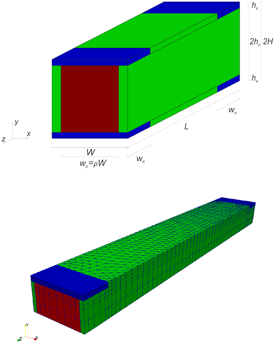
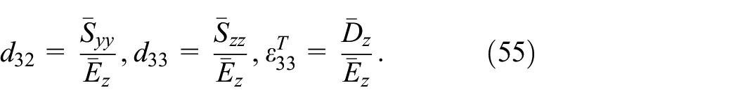
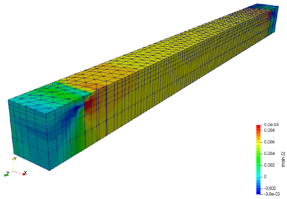
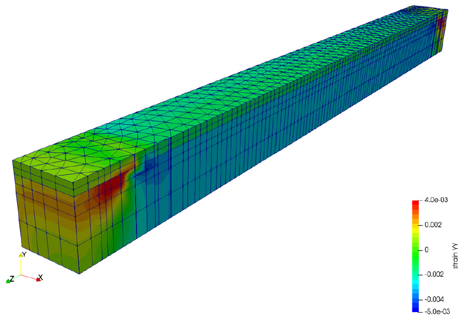
5.3. Poling of a $d_{33}$ macro fiber composite

As an advanced numerical example, we consider a $d_{33}$ macro fibre composite ( $d_{33}$ MFC). Such a $d_{33}$ MFC is commercially available e.g. from Smart Materials Corp., Sarasota, FL. This MFC consists of thin (microscopic) fibres of PZT which are aligned in an epoxy matrix. Interfingering copper electrodes are aligned at the top and bottom at an angle of ${90}^{°}$ . The computation of macroscopic material constants resembling the mircostructure has been addressed in the literature in different contributions. Analytic mixing rules for a simplified setup were provided by Deraemaeker et al. (2009). In Deraemaeker and Nasser (2010), the authors address the fact that the geometric setup of the $d_{33}$ MFC leads to non-uniform polarization directions in three dimensions. However, they did not simulate the polarization process, but assumed the remanent polarization to be of uniform absolute value $P_0$ , but in direction of the electric field. Shindo et al. (2011) presented a first simulation of the polarization process, but using a different model from the one proposed in this work, and only in two space dimensions. Our contribution is now a complete simulation of the poling process, where a poling electric field of size $3E_0$ is applied to the interdigitated electrodes. Afterwards, using this remanent polarization field, a small voltage is applied. Strain and dielectric displacement computed in this linear problem then lead to macroscopic $d_{33}$ , $d_{32}$ and ${\epsilon }_{33}^T$ constants.

A sketch of the unit cell as used by Deraemaeker and Nasser (2010) is provided in Figure 5. Conforming with Shindo et al. (2011), we use $W=206.95\mu \mathrm{m}$ for the width of an epoxy/PZT fibre set. The width of the PZT fibre $w_p$ is then defined by the volume ratio $\rho$ of the fibre. We use $\rho =0.86$ , which implies $w_p=\rho W=177.977\mu \mathrm{m}$ . Height of fibre and electrode are also taken from Shindo et al. (2011), and set to $2h_p=206.40\mu \mathrm{m}$ and $h_e=18\mu \mathrm{m}$ . To compare our results to the values provided by Deraemaeker and Nasser (2010), we use their settings $w_e=h_p$ for the width, and $L/H=12$ for the distance of the copper electrodes. This implies $w_e=103.20\mu \mathrm{m}$ and $L=1454.40\mu \mathrm{m}$ .

Figure 5.

Homogenization of macro fibre composite: schematic sketch of unit cell and finite element mesh consisting of 6360 prismatic elements.

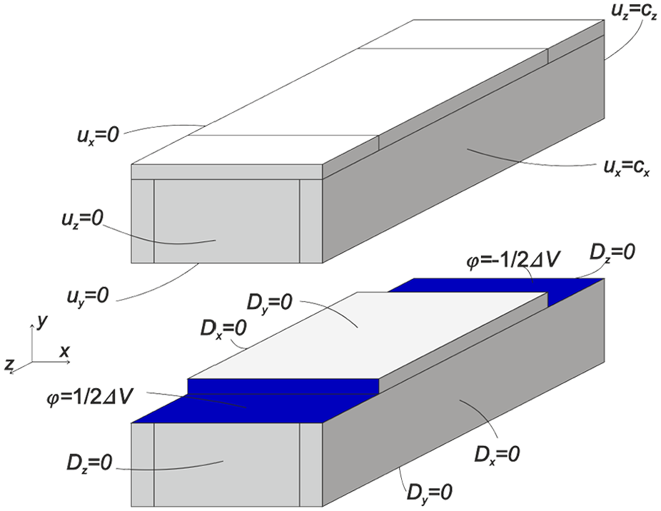
Due to symmetry of the geometry and the applied load, which is an applied voltage to the electrodes, we may consider one half of the geometry only. Boundary conditions are defined in Figure 6. While the displacement boundary conditions are straightforward for this symmetric problem, we shortly comment on the electric boundary conditions. On the copper electrodes, we assume a constant electric potential of $\phi =\pm \mathrm{\Delta }V$ . This is realized in the following way in our mixed finite element formulation: dielectric displacements are not modelled in the electrode volume, but only in the PZT and epoxy parts. On the electrode surfaces, which are now surfaces of the electric domain, the potential boundary condition $\phi =\pm \frac{1}{2}\mathrm{\Delta }V$ is applied via a surface integral in the external work statement (6). On all other surfaces, surface charges $\mathbf{D}·\mathbf{n}$ are set to zero.

Figure 6.

Homogenization of macro fibre composite: symmetry boundary conditions posed on eigth of unit cell, top: displacement boundary conditions, bottom: electric boundary conditions.

The choice of material parameters was conducted in the following way: All constants that could be re-used from the linear model by Deraemaeker et al. (2009); Deraemaeker and Nasser (2010) were used. This includes the linear properties of epoxy ( $Y_E=2.9\mathrm{GPa}$ , $\nu =0.3$ , $\epsilon =4.25{\epsilon }_0$ ) and copper ( $Y_E=117\mathrm{GPa}$ , $\nu =0.31$ ). In this example, we assume that the stiffness at constant electric field ${\mathbf{c}}^E$ is constant and isotropic, and defined by Young’s modulus $Y_E$ and Poisson ratio $\nu$ . The permittivity at constant stress is assumed constant isotropic at ${\epsilon }^T=1900{\epsilon }_0$ . Further, the additive part of the free energy function ${\hat{\psi }}^i$ is chosen such that its derivative needed in implementations reads

$${\hat{\psi }}^i({\mathbf{P}}^i)=\frac{h_0{P}_0}{2|{\mathbf{P}}^i|}\left(\log \left(\frac{P_0+|{\mathbf{P}}^i|}{P_0-|{\mathbf{P}}^i|}\right)\right){\mathbf{P}}^i.$$

(54)

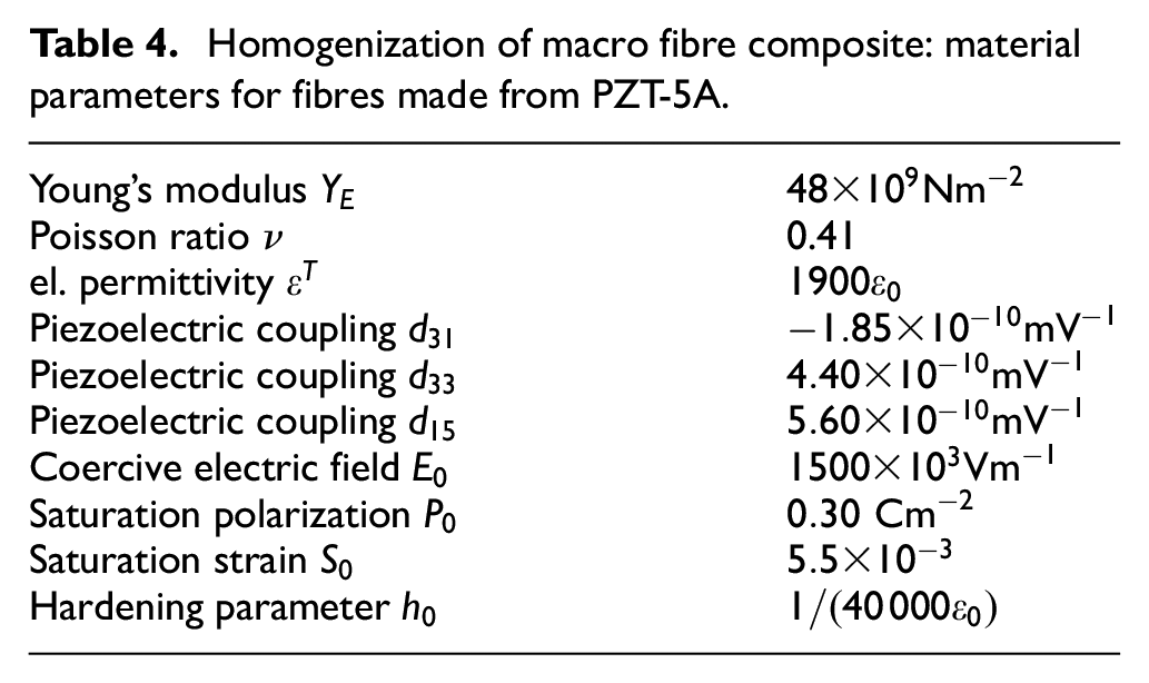
The coercive electric field $E_0$ , saturation polarization $P_0$ and remanent saturation strain $S_0$ are taken from Shindo et al. (2011). The hardening parameter for PZT-5a was chosen such that the hysteresis measurements depicted in (Hooker, 1998, Figure 7(d)) could be reproduced. The regularization parameter for the dissipation function was chosen as $\epsilon ={10}^{-4}{P}_0$ , and to avoid convergence problems at the singularity at the electrode also ${\hat{\psi }}^i$ was regularized using the same parameter. All material parameters are also provided in Table 4.

Figure 7.

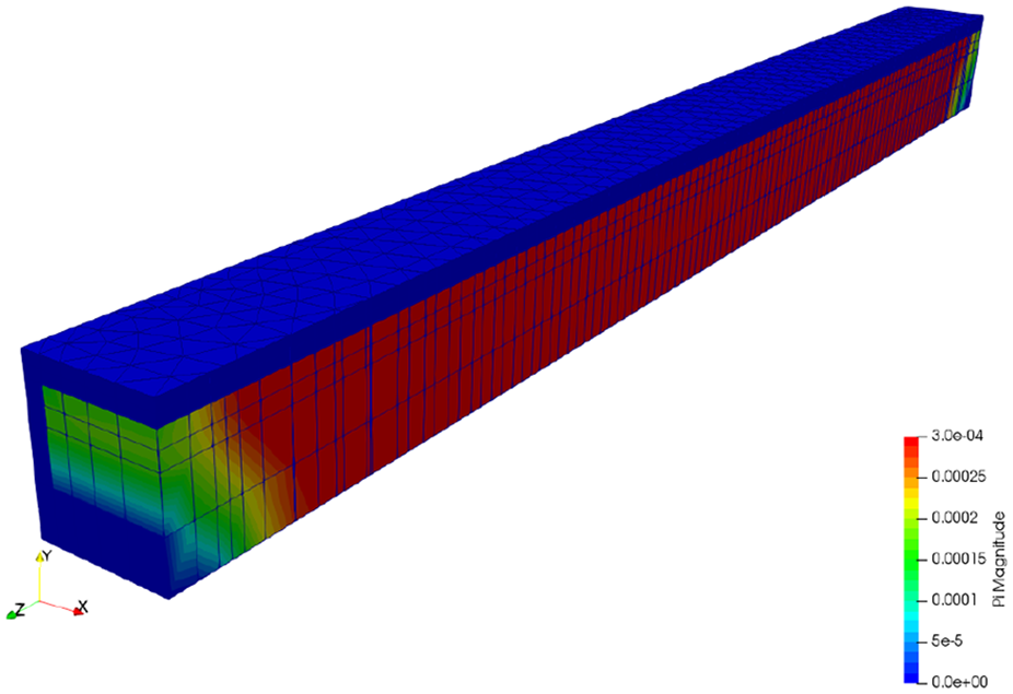
Homogenization of macro fibre composite: remanent polarization at full poling electric field $3E_0$ . The unit cell is virtually cut in half at $x=W/2$ .

Table 4.

Homogenization of macro fibre composite: material parameters for fibres made from PZT-5A.

Young’s modulus $Y_E$	$48\times {10}^9{\mathrm{Nm}}^{-2}$
Poisson ratio $\nu$	0.41
el. permittivity ${\epsilon }^T$	$1900{\epsilon }_0$
Piezoelectric coupling $d_{31}$	$-1.85\times {10}^{-10}{\mathrm{mV}}^{-1}$
Piezoelectric coupling $d_{33}$	$4.40\times {10}^{-10}{\mathrm{mV}}^{-1}$
Piezoelectric coupling $d_{15}$	$5.60\times {10}^{-10}{\mathrm{mV}}^{-1}$
Coercive electric field $E_0$	$1500\times {10}^3{\mathrm{Vm}}^{-1}$
Saturation polarization $P_0$	$0.30{\mathrm{Cm}}^{-2}$
Saturation strain $S_0$	$5.5\times {10}^{-3}$
Hardening parameter $h_0$	$1/(40000{\epsilon }_0)$

In Figure 7 the absolute value at full poling electric field $3E_0$ is depicted. For better visualization, the unit cell is virtually cut in half at $x=w/2$ . Figures 8 and 9 show the strain distributions of $S_{\mathrm{yy}}$ and $S_{\mathrm{zz}}$ , respectively. After the poling field was removed, a linear computation was performed to compute the homogenized material constants. To this end, an electric potential was applied to the electrodes, and the macroscopic material constants $d_{32}$ , $d_{33}$ and ${\epsilon }_{33}^T$ were computed by the following formulae provided by Deraemaeker and Nasser (2010),

$$d_{32}=\frac{{\overline{S}}_{\mathrm{yy}}}{{\overline{E}}_z},d_{33}=\frac{{\overline{S}}_{\mathrm{zz}}}{{\overline{E}}_z},{\epsilon }_{33}^T=\frac{{\overline{D}}_z}{{\overline{E}}_z}.$$

(55)

The average values of ${\overline{S}}_{\mathrm{yy}}$ and ${\overline{S}}_{\mathrm{zz}}$ were derived from the constant displacements arising at the boundaries, compare Figure 6, ${\overline{S}}_{\mathrm{yy}}=c_x/W$ and ${\overline{S}}_{\mathrm{zz}}=c_z/L$ . The average value of the electric field was chosen according to Deraemaeker and Nasser (2010) as ${\overline{E}}_z=\mathrm{\Delta }V/L$ . The average value of the dielectric displacement was chosen as the total charge at one electrode divided by the cross section area $2\mathrm{WH}$ . The values we found in our computations are listed in Table 5. The values are compared to the constants derived by the analytic mixing rules from Deraemaeker et al. (2009) as well as to constants computed by Deraemaeker and Nasser (2010) in their finite element setup. There are several facts possibly contributing to this outcome: first, the absolute value of the polarization always stays below saturation polarization. It decreases slightly more as the poling electric field is reduced in the used material law, as the remanent polarization at zero voltage is below the saturation polarization also in one-dimensional settings. Moreover, the polarization is lower close to the fibre boundaries, where the interface to the epoxy matrix is located. And last, in the zones below the electrodes, the electric field and polarization are not oriented in z direction, but rather in vertical x direction. This last issue has also been discussed in the finite element simulation by Deraemaeker and Nasser (2010).

Figure 8.

Homogenization of macro fibre composite: transverse strain $S_{\mathrm{yy}}$ at full poling electric field $3E_0$ . The unit cell is virtually cut in half at $x=W/2$ .

Figure 9.

Homogenization of macro fibre composite: longitudinal strain $S_{\mathrm{zz}}$ at full poling electric field $3E_0$ . The unit cell is virtually cut in half at $x=W/2$ .

Table 5.

Macroscopic material constants for the $d_{33}$ MFC. Mixed FE denotes results from the present contribution, mixing rules denotes the analytic values from Deraemaeker et al. (2009), FE ref. are values estimated from the plots provided by Deraemaeker and Nasser (2010) for their finite element computations.

	$d_{32}({\mathrm{nmV}}^{-1})$	$d_{33}({\mathrm{nmV}}^{-1})$	${\epsilon }_{33}^T$
Mixed FE	$-134.4$	$366.8$	$2162{\epsilon }_0$
Mixing rules	$-176$	$436$	$1593{\epsilon }_0$
FE ref.	$-169$	$422$	$1600{\epsilon }_0$

6. Conclusion

In this contribution, we have presented energy-based model of the ferroelectric polarization process. In an energy-based setting, dielectric displacement and strain (or displacement) are the primary independent unknowns, while the remanent polarization vector is added as an internal variable. Electric field and stress are evaluated through post-processing utilizing the material law. The model is governed by two constitutive functions: the free energy function and the dissipation function. We provide standard choices from the literature for the free energy, and motivate our choice of dissipation function. As it is non-differentiable, we proposed to regularize the problem. Then, a variational equation can be posed, which is subsequently discretized using conforming finite elements for each quantity. One section is devoted to the finite elements, as non-standard continuity is needed for the dielectric displacement to obtain a conforming method. We provide corresponding finite elements, that are chosen such that Gauss’ law of zero charges is satisfied exactly. The discretized variational equations are solved for all unknowns at once in a single Newton iteration. We present numerical examples gained in the open source software package Netgen/NGSolve.

An extension to models including ferroelasticity in the sense of Landis (2002), Klinkel (2006) or Semenov et al. (2010) seems feasible. Concerning the theoretical aspects, the extension is straightforward, and has been considered in our paper Pechstein et al. (2020). An implementation of these more involved energies is planned in upcoming contributions.