Sage Journals: Discover world-class research

Abstract

Active piezoelectric transducers are successfully deployed in recent years for structural health monitoring using guided elastic waves or electro-mechanical impedance (EMI). In both domains, damage detection can be hampered by operational/environmental conditions and low-power constraints. In both domains, processing can be divided into approaches (i) taking into account baselines of the pristine structure as reference, (ii) ingesting an extensive measurement history for clustering to explore anomalies, (iii) incorporating additional information to label a state. The latter approach requires data from complementary sensors, learning from laboratory/field experiments or knowledge from simulations which may be infeasible for complex structures. Semi-supervised approaches are thus gaining popularity: few initial annotations are needed, because labels emerge through clustering and are subsequently used for state classification. In our work, bending and combined bending/torsion studies on rudder stocks are considered regarding EMI-based damage detection in the presence of load. We discuss the underpinnings of our processing. Then, we follow strategy (i) by introducing frequency warping to derive an improved damage indicator (DI). Finally, in a semi-supervised manner, we develop simple rules which even in presence of varying loads need only two frequency points for reliable damage detection. This sparsity-enforcing low-complexity approach is particularly beneficial in energy-aware SHM scenarios.

Keywords

Structural health monitoring electro-mechanical impedance signal processing dynamic frequency warping machine learning

1. Introduction

The capability of a technical structure for example, to assess its health state, turns it into an intelligent (or smart) structure. Such a self-assessment aims at avoiding disaster, increasing operational availability, or facilitating maintenance. The assessment of health may be enabled through monitoring. The function of structural health monitoring (SHM) is at the most basal level the detection of damage. Although localization or even damage quantification are subject to current research efforts, defect detection remains sufficient in most practical circumstances for achieving the aforementioned aims (Fritzen and Kraemer, 2009).

For SHM employing both guided elastic waves (GEW) or the electro-mechanical impedance (EMI) method, active piezoelectric transceivers (Giurgiutiu, 2014; Lammering et al., 2017; Mueller, 2017) have already been utilized productively in the past in a broad range of scenarios. They actively induce a forced local excitation in order to inspect a particular region of a structure. Studies using active piezoelectric elements include the EMI spectroscopy of grouted connections which are widely seen in offshore structures (Moll, 2019), sensor fault detection using the EMI method (Mueller and Fritzen, 2017), EMI-based sensing of bones in medical settings (Moll et al., 2019a; Srivastava et al., 2017) as well as GEW-based identification of delaminations in composites (Migot et al., 2021), multi-site damage imaging with GEW (Neubeck et al., 2020) or GEW-based defect localization including size assessment (Memmolo et al., 2018).

Commonly the active piezoelectric transducer is directly and permanently integrated into the structure’s material (Bosse et al., 2018). Therefore SHM-related signal processing is frequently restricted by limited power resources during operation and/or low-complexity hardware (Kexel et al., 2020; Salehi et al., 2021; Tang et al., 2010; Zonzini et al., 2021). The demand for identifying the most informative variables and thus for processing of only a reduced amount of data has been answered with introduction of sparsity-promoting approaches in the last decades (Efron and Hastie, 2016; Hage et al., 2020; Hastie et al., 2015).

Prescinding from resources issues and complexity constraints, an intelligent structure will typically experience changing environmental and operational conditions (EOC) during its life span, such as load, moisture, or temperature. Both for GEW (Douglass and Harley, 2020; Kexel et al., 2021; Moll et al., 2019b; Salas et al., 2018) as well as the EMI technique (Lim et al., 2021; Neuschwander et al., 2019; Wandowski et al., 2017) the presence of EOC can significantly exacerbate SHM-related signal processing. The large diversity in EOC may complicate damage detection. Traditionally, SHM approaches consider a set which encompasses baseline measurements of the intact structure for comparison with the later readings, in order to discover defects from the later readings. But facing a variety of EOC the reference set has to grow substantially which may render this traditional approach impractical. Likewise, EOC pose also a severe obstacle for approaches using the so-called relative baseline concept (Jung et al., 2014) which omits historical baselines but draws on data from other likely undamaged regions of the structure as references.

In order to alleviate the influence of EOC in SHM applications, a couple of compensation methods have been proposed (Croxford et al., 2010; Douglass and Harley, 2018; Tekkalmaz et al., 2020; Wandowski et al., 2017) which involve different types of searches for an optimal alignment. In contrast to static distances, such as root-mean-square deviation, mean absolute distance (MAD), correlation coefficient (Tekkalmaz et al., 2020) or cumulative power (Soman et al., 2020), here distances that originate from a dynamic process, like optimization and/or search, are referred to as a dynamic distance.

Besides EOC compensation, another aspect that is touched upon in the present work concerns the overall signal processing strategy in the SHM framework. In general, SHM shares some challenges with other statistical or machine learning approaches where the witnessed successes over the last decades are partly due to the availability of enormous amounts of so-called labeled (or annotated) data (Deng et al., 2009; Lin et al., 2014; Rautela et al., 2021). However, acquiring data and assigning labels oftentimes becomes laborious, since it requires supervision and additional knowledge for example, about the current state of the structure of interest. In the SHM framework and similar settings (Bergmann et al., 2019), labeling implies to manually and explicitly declare the structure of interest, for example, as healthy or damaged. In many circumstances it remains less intricate to merely retrieve unlabeled data without extensive context. Semi-supervised approaches (Sheikhpour et al., 2017) intend to mitigate the necessity for labeled data by leveraging unlabeled data.

In the present work, previous studies on bending (Moll et al., 2020a) and combined bending with torsion (Moll et al., 2020b) are complemented. They consider rudder stocks which are frequently encountered in the maritime industries. The task of EMI-based defect detection is performed in spite of applied loads. In particular, the contribution of the present work consists in the following achievements:

We analyze data acquired from two distinct engineering structures, make use of a comprehensive toolbox of statistical methods and present in-depth results considering inputs from a range of sensors.

We theorize about the decomposition of the susceptance spectrum in order to be able to better separate effects of load and damage.

We introduce a frequency-warping approach for the derivation of an enhanced numerical damage indicator (DI) based on the dynamic distance with respect to the baseline readings.

We explore a semi-supervised approach by reconciling on the one hand unsupervised cluster analysis for discovering annotations and on the other hand a supervised low-complexity tree classifier which leads in sum to a reliable damage detector requiring only two frequency points.

The remainder of this work is organized as follows: Section “Methodology” explains the used signal processing approaches including EMI spectroscopy, Section “Setup” deals with the experimental arrangement of the considered studies, Section “Results and Discussion” covers experimental outcomes, their analysis including the corresponding findings and Section “Conclusions” provides a summary as well as an outlook.

2. Methodology

Since a collection of statistical tools will be employed in this work, the methodological underpinnings for data analysis are provided in this section including some background on the EMI method.

2.1. Binary classification and classification trees

Defect detection represents a fundamental task in SHM. It is frequently cast into a decision concerning the two classes “pristine” or “damaged.” Typically, the decision rests upon one feature, namely a suitable continuous variable, dubbed DI, whose numerical range is split into two disjunct portions using a constant (or threshold): values of the DI below the threshold are classified as “pristine” and the remaining as “damaged.” In order to assess a binary classification approach having a given threshold, the true and false positives as well as the true and false negatives among the data points are assembled into a so-called confusion matrix (Rautela et al., 2021). More general, in order to choose an optimal threshold or to assess the fundamental trade-off between true and false positives by considering all possible thresholds, the Receiver Operating Characteristic (ROC) curve can be consulted which describes the true positive rate $p_{TP}$ as a function of the false positive rate $p_{FP}$ . ROC curves also enable the performance comparison of two competing DIs. The ROC curve’s area-under-curve (AUC) represents a widely used figure-of-merit which is closely tied to statistical hypothesis testing (Hastie et al., 2009). AUC has a value between 0 and 1 where 1 indicates a perfect binary classifier. Like any other area under a curve $y (x)$ , AUC can be calculated through integration:

AUC = \int_{0}^{1} y (x) d x

(1)

where $x = p_{FP}$ and $y = p_{TP}$ .

Mathematically speaking, tree classifiers (Loh, 2011) are a natural extension of the binary classification problem: They partition the value range of one feature also using a simple threshold, even tough they will typically undergo several iterations (or binary splits) to generate more than two partitions. Furthermore, they cover commonly a feature space with more than one feature. The decision where to split the value range of a feature optimally with a threshold, can rely on different metrics, such as the misclassification rate or the Gini coefficient (Hastie et al., 2009; Loh, 2011). Tree classifiers are especially appealing, because their output can readily be interpreted by humans and lead therefore to an improved traceability of statistical decisions, for example, for damage detection in SHM (see Figure 1 for an illustrative example). In order to prevent overfitting but keeping the essential structure of the feature space, the number of splits in a classification tree can be limited by so-called pruning. Furthermore, the importance of certain features (or predictors) can also be estimated by using trees. Predictor importance helps to identify the most informative selection of features. Predictor importance can be evaluated with a tree model even in the presence of correlated predictors, by employing curvature and interaction tests. These tests determine association between predictors as well as interaction between a pair of predictors with the response variable (Loh, 2002). For example, the susceptance at one frequency point in the spectrum will likely be strongly correlated with the susceptance value at an adjacent frequency.

Figure 1.

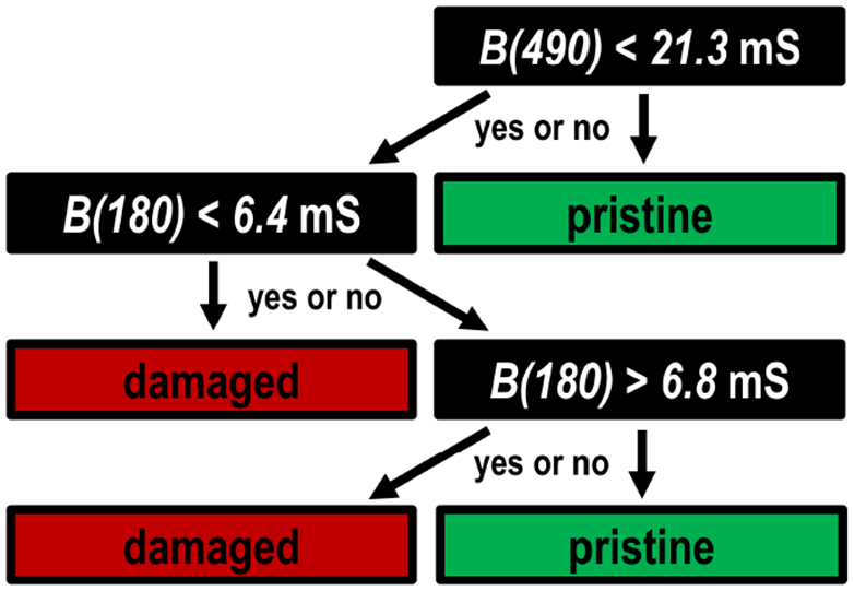
Exemplary classification tree with illustrative numerical values which are however actually later on in this manuscript used in the joint bending/torsion study for discriminating between damaged and pristine states for transducer T2. The susceptance at a frequency of for example, 180 kHz is denoted in italic font by $B (180)$ . Accordingly, the matrix of susceptance measurements is written in bold italic font as $B$ elsewhere.

2.2. Principal components and cluster analysis

If the class labels are available, tree classifiers are a convenient way of capturing the most informative aspects of the data with simple rules. However, also in a setting with unlabeled data, there exist approaches for exploration of the data’s essential structure (Park et al., 2008). Principal component analysis seeks a set of projections (or linear approximations to the data) which are ordered according to variance and which are uncorrelated. Singular value decomposition (SVD) is the standard numerical approach to arrive at the principal components. The SVD of the data matrix $B$ with $n \times m$ entries, for example, $n$ susceptance spectra each having $m$ frequency points, reads as:

B = U \cdot D \cdot V^{T}

(2)

The matrices $U$ and $V$ are orthogonal with size $n \times m$ and $m \times m$ , respectively, whereas $D$ is a diagonal matrix of size $m \times m$ . Its entries $d_{i}$ are dubbed singular values. By omitting a scaling factor of $n$ , the covariance of the data matrix can be written as:

B^{T} \cdot B = V \cdot D^{2} \cdot V^{T}

(3)

This factorization represents the eigendecomposition of $B^{T} \cdot B$ where the columns of $V$ are the eigenvectors $v_{j}$ . The vector $z_{i} = B \cdot v_{i}$ is dubbed $i$ -th principal component having the $i$ -th largest variance amongst the normalized linear combinations of the columns of data matrix $B$ . The concept of the so-called explained variance is a way to quantify the contribution of each principal component: it captures the fraction of variance this component exhibits relative to the total variance of the whole data set. Hence, if data can be well approximated by just the first principal component only, then this component will have an explained variance of close to 100% (Hastie et al., 2009).

Using SVD and the principal components can help to explicate clusters in the feature space. However, cluster analysis can still be accomplished without prior decomposition, namely when relying solely on the pair-wise dissimilarity between measurements. For example, the dissimilarity between a baseline and subsequent measurements, has already been discussed regarding DIs.

Hierarchical clustering are classical approaches which are highly interpretable. The standard approach is Ward’s method (Romesburg, 2004; Ward, 1963). Hierarchical clustering produces tree-like representations (dendrograms) in which the clusters at a higher level inside the tree are formed by merging clusters at a lower level. At the highest level just one cluster contains the complete data set. At the lowest level, each cluster encompasses only one measurement. So-called agglomerative approaches begin at the lowest level. The pair chosen for merging consist of the two groups with the smallest intergroup dissimilarity. Therefore, a measure of dissimilarity between two clusters, dubbed $C_{i}$ and $C_{j}$ , has to be established which reads as follows for method:

r (C_{i}, C_{j}) = \frac{1}{n_{C_{i}} \cdot n_{C_{j}}} \sum_{i \in C_{i}, j \in C_{j}} r (i, j)^{2}

(4)

where $n_{C_{i}}$ and $n_{C_{j}}$ are the number of measurements in the corresponding cluster and $i$ as well as $j$ denote indices of measurements belonging to $C_{i}$ or $C_{j}$ , respectively, which have distance $r (i, j)$ .

Arriving at a full dendrogram, the task of choosing a natural clustering, that is, the optimal number of clusters $\tilde{N}$ , has to be dealt with. The silhouette coefficient $S (N)$ allows for an automated choice of the natural number of clusters by finding the largest silhouette coefficient:

S (\tilde{N}) = max_{N \in {2, . . .}} S (N)

(5)

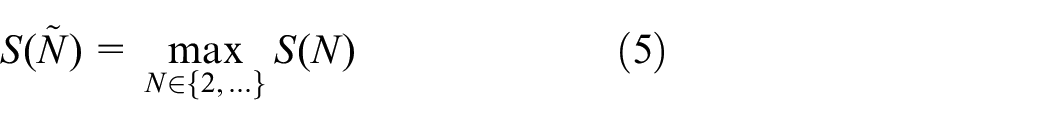
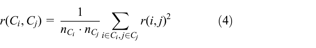
For a given number of clusters $N$ , the silhouette coefficient is the average over all measurements $i$ of which each has its individual coefficient $s_{i}$ :

S (N) = \frac{1}{n} \sum_{i}^{n} s_{i} = \frac{1}{n} \sum_{i}^{n} \frac{b_{i} - a_{i}}{max (b_{i}, a_{i})}

(6)

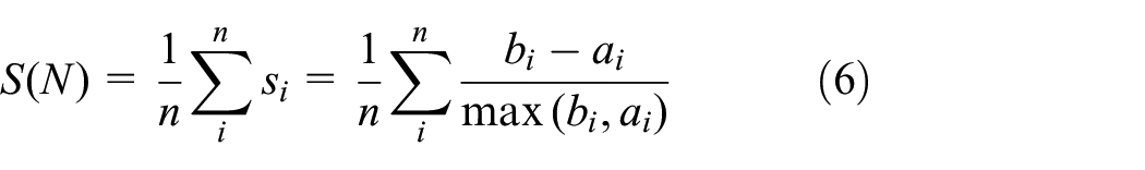
Here, $a_{i}$ represents the average distance from measurement $i$ to all remaining measurements $j$ in its own cluster $C_{i}$ :

a_{i} = \frac{1}{n_{C_{i}} - 1} \sum_{j \in C_{k}, i \neq j} r (i, j)

(7)

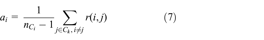
Moreover, $b_{i}$ represents the average distance from measurement $i$ to all measurements $k$ in another cluster $C_{k}$ where $C_{k}$ is the cluster with the smallest average distance:

b_{i} = min_{i \neq k} (\frac{1}{n_{C_{k}}} \sum_{j \in C_{k}} r (i, j))

(8)

2.3. Dynamic frequency warping compensation

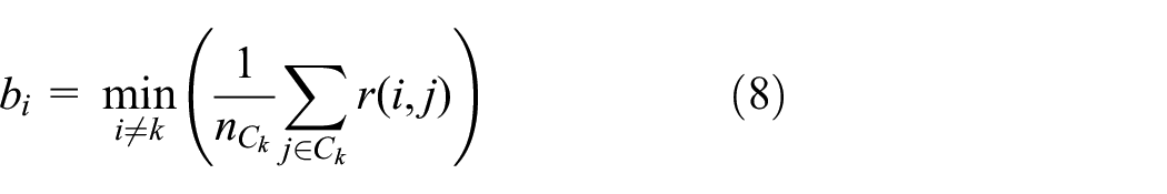
In general, dynamic warping is beneficial for seeking an optimal alignment between two sequences which share some common signatures but are for example, shifted in a non-trivial manner. Warping will match both sequences with elementary manipulations and the resulting dynamic distance hence indicates to which extent both sequence actually do not match despite the performed elementary manipulations. Related methods have been widely adopted for biological sequence alignment (Needleman and Wunsch, 1970). Amongst many other, applications of dynamic warping include GEW temperature compensation in the time domain (Douglass and Harley, 2018). Moreover, frequency warping has been considered for aligning voice spectra (Neuburg, 1988; Toda et al., 2001). In the present work, one sequence is the susceptance spectrum at some point in time and the second sequence is a baseline spectrum. Figure 2 covers an idealized and illustrative example.

Figure 2.

Exemplary warping of idealized susceptance spectra. When load damps the spectrum’s slope, the distance between spectra with/without load is significant whereas the dynamic distance after warping almost completely compensates the effect of load. The inset shows a magnification where the step-like curve shows the good but not perfect compensation.

Each frequency point of the one sequence will be aligned with the frequency points of the baseline. The optimization procedure for the mapping is constraint so as to yield a plausible alignment: susceptance spectra naturally start at the origin, that is, small frequency coincides with a small susceptance, and during optimization for each sequence a frequency point is allowed to be shifted only to a higher frequency or stay untouched. This is usually referred to as monotonicity criterion. The above constraints enforce that no frequency point is skipped or that parts of the susceptance signature are repeated. In particular, dynamic warping is carried out using the following steps:

Assignment of local and global penalties,

Dynamic programming and backtracking,

Sequence alignment.

In order to guide the optimization later on through an objective function, a local penalty has to be defined for the elementary manipulations. The local penalty is equal to the distance of the points. Ideally, evaluating the globally optimal warping path calls for the enumeration of every feasible path which is however impractical. Therefore, for the all-to-all mapping a global penalty is assigned which is equal to the sum of the local penalties. The iterative approach, dubbed dynamic programming, breaks the problem down into sub-problems. The approach recursively constructs the global penalty scheme by deducing each instance based on neighboring global penalty. When the global penalty scheme is fully constructed, the optimal warping path is found using so-called backtracking. Beginning at the minimal global penalty, it hops to adjacent mappings having minimal global penalty. Knowing the optimal path, that is, the optimal mapping between the sequences, both spectra can finally be aligned.

2.4. Electro-mechanical impedance spectroscopy

When actuated by a constant voltage, an attached piezoceramic transducer will act with constant force on the host structure according to the inverse piezoelectric effect. Regarding the EMI technique, transducers are excited in a harmonic manner with alternating voltage and hence lead to a harmonic force. The electrical impedance of a piezoelectric element is linked to the mechanical impedance of the structure. The structural response expresses itself with a distinct signature in the electro-mechanical admittance spectrum. The admittance signature depends on the stiffness and damping of the host structure, the dimensions as well as orientation of the transducer. The admittance

Y = G + ι \cdot B

(9)

consists of conductance $G$ (real part) and its imaginary part, dubbed susceptance $B$ . The changes in the admittance signature are indicative of the presence of structural damages (Moll, 2019; Mueller and Fritzen, 2017).

The signature of the susceptance spectrum is the outcome of an interplay of the transducer’s and the structure’s material properties. Through the numerical study regarding the influence of different material parameters on the susceptance spectrum (Madhav, 2007), two major effects have been identified, namely changes in slope and shifts in the peaks. This theoretical observation forms the bedrock for the discussion hereafter. EOC can have a complicated influence on the underlying material properties and eventually on the susceptance spectrum. For previous experiments on a watercraft rudder stock an approximately linear relationship could be uncovered between slope of the susceptance and a change in termperature (and load) (Neuschwander et al., 2019). During monitoring studies on a reinforced concrete beam regarding the effect of long-term dynamic loading a so-called equivalent stiffness of the structure has been derived from the slope of the susceptance (Kaur et al., 2019): Here, fatigue and the emergence of microcracks, which represents an inevitable operational condition, could be associated with a decrease in the slope. Furthermore, the curing of concrete has been associated with reduction in the slope of the imaginary component of the admittance signature spectrum, that is, susceptance, (Lim et al., 2021). Sensor breakage and sensor debonding has been reported to lead to a decrease and increase of the susceptance slope, respectively (Overly et al., 2008). Apart from considering the slope, susceptance signatures have been found to be suitable for delamination detection in composite structures, however in the absence of loads; moreover susceptance has been described for indicating axial or transversal loads, however in the absence of damage; an important challenge to be addressed regarding the EMI technique is about the damage detecion performance if both damage and loads prevail concurrently (Annamdas and Soh, 2010). Lastly, it is important to stress that the distinct choice of transducer configuration can have a decisive impact on how a damage will alter the susceptance spectrum (Kaur et al., 2017).

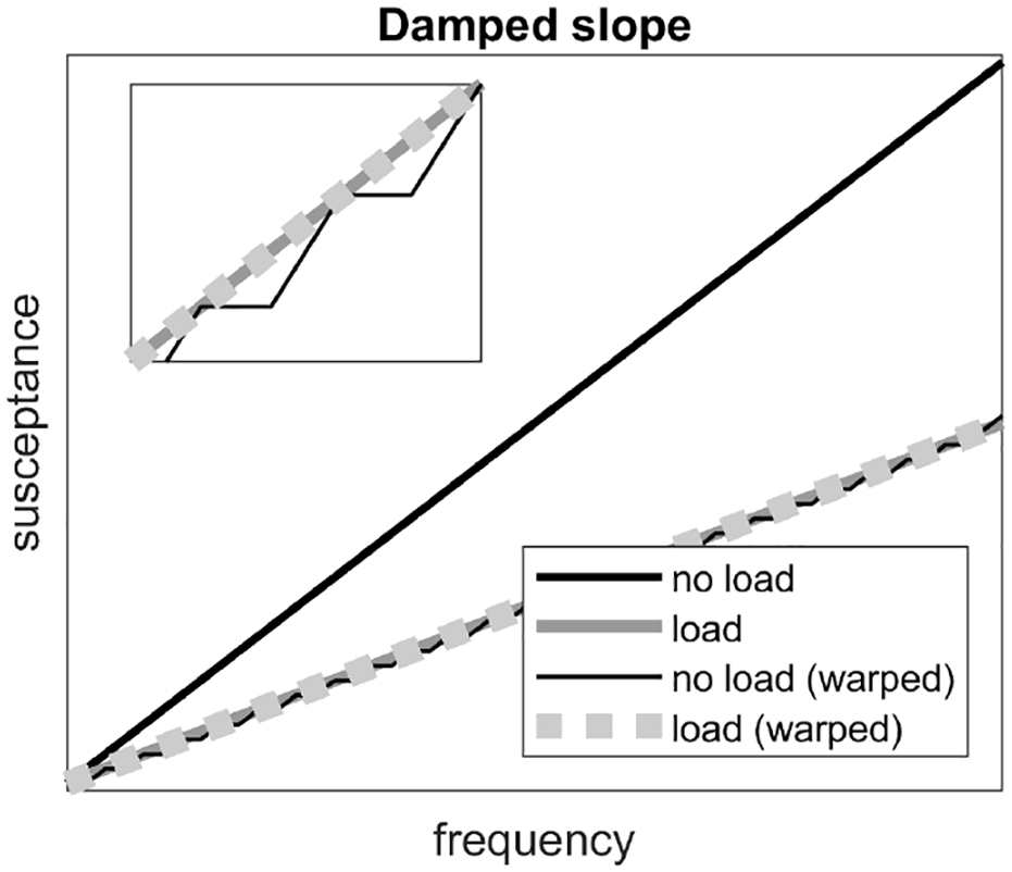
In Figure 3 a connection between EOC (or the two major effects, i.e. slope and peak changes) and the principle components of susceptance measurements is drawn. The susceptance spectrum is stylized into one oscillation representing one peak and the general linear trend line. Variations in slope and shifts in the peak position will hence lead to two significant principal components where the first component, that is, an approximately linear function, mostly captures variations in slope and the second component exhibits more complicated behavior.

Figure 3.

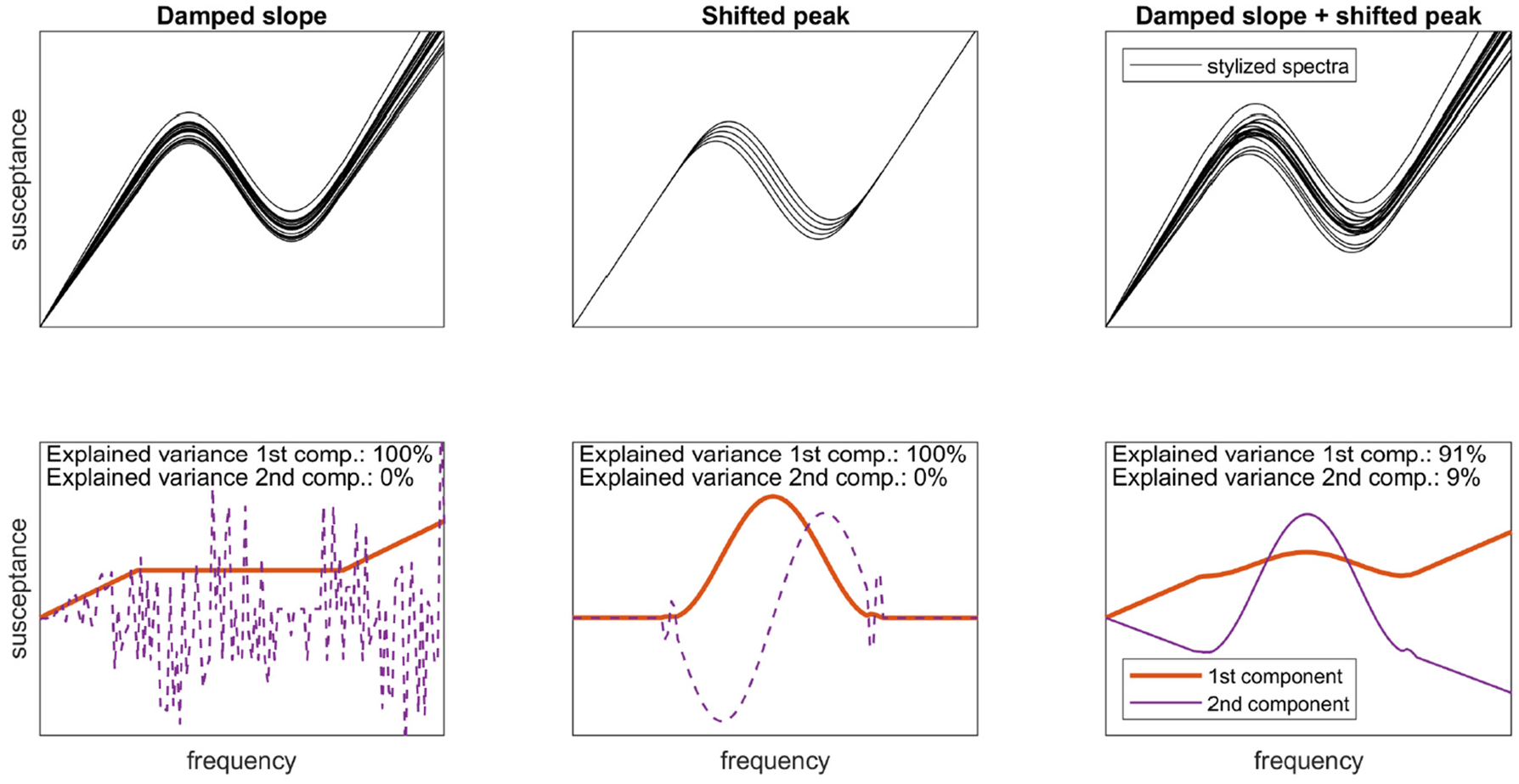
Stylized spectra (top row) and their decomposition (bottom row). A variation in the overall slope (left column) or in the peak position (middle) can each be explained by one component only. A variation in both (right column) renders two components necessary. Here, the first component goes mainly linear with the frequency whereas the second component reveals oscillations in the order of the peak width.

3. Setup

Details of the experimental setup regarding the first study on bending and of the second study combining bending with torsion can be found in (Moll et al., 2020a) and (Moll et al., 2020b), respectively. For the sake of completeness, the essential facts are however re-stated here.

3.1. Bending study

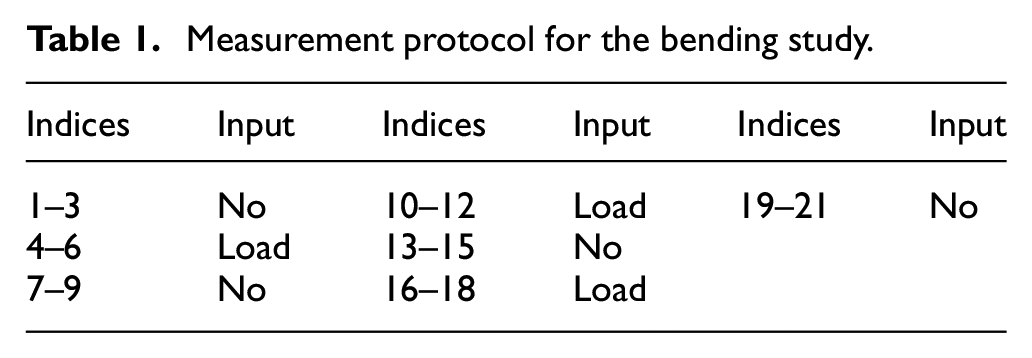
The scaled prototype rudder stock having a reduced size and a total length of 2000 mm is depicted on the left-hand side of Figure 4. Its maximal diameter is 206 mm. A mix of materials involving carbon-fiber reinforced plastics (CFRP) as well as steel is used. The rudder stock is designed so as to replace conventional all-steel specimens in the future. Therefore, some portions still must remain to be composed of steel, because steering gear and rudder blades are conventionally fixed to the rudder stock with conical press-fit connections and conical press fits must not be made out of CFRP due to enormous local surficial loads. CFRP cones will not reliably bear those loads, because of the comparatively small stiffness and radial strength as well as because of the creep of the resin. A double-lapped shear conjunction using hardened steel pins links the CFRP middle-portion and the metallic ends. A nominal bending load of 282 kN is applied in the laboratory experiments whose measurement protocol is provided in Table 1. A total of $n = 21$ measurements has been performed, including three repetitions of measurements for each of the subsequently investigated states of the structure. The defect that has to be identified is not artificial or extrinsic, but is induced by surpassing the critical mechanical load. The result is a pin failure, that is, a plastic deformation of the metal pins. Strain gages (HBM 1-LI66-10/350) and piezoceramic transducers (PIC 255, diameter of 10 mm, thickness of 0.25 mm) are employed. The transducers are attached with HBM X60 glue and are distributed over the circumference of the rudder stock. The transducers are connected to multichannel EMI device with TiePie Handyscope HS5 and an PiezoDrive PD200 amplifier. From the EMI literature, it is apparent that the considered frequency range is dependent on the particular EMI application (Tenreiro et al., 2021). The range from 25 to 500 kHz considered here contains the frequencies that are also relevant in other similar studies (Lim et al., 2021; Mueller, 2017; Neuschwander et al., 2019; Soman et al., 2020).

Figure 4.

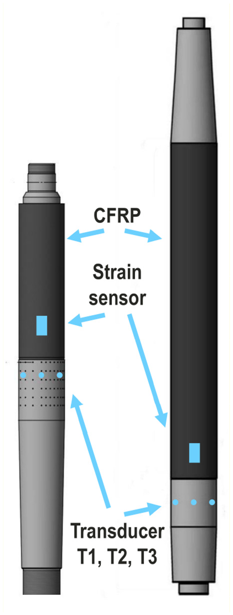
Rudder stock for the bending study (left) and for the combined bending/torsion study (right).

Table 1.

Measurement protocol for the bending study.

Indices	Input	Indices	Input	Indices	Input
1–3	No	10–12	Load	19–21	No
4–6	Load	13–15	No
7–9	No	16–18	Load

3.2. Combined bending/torsion study

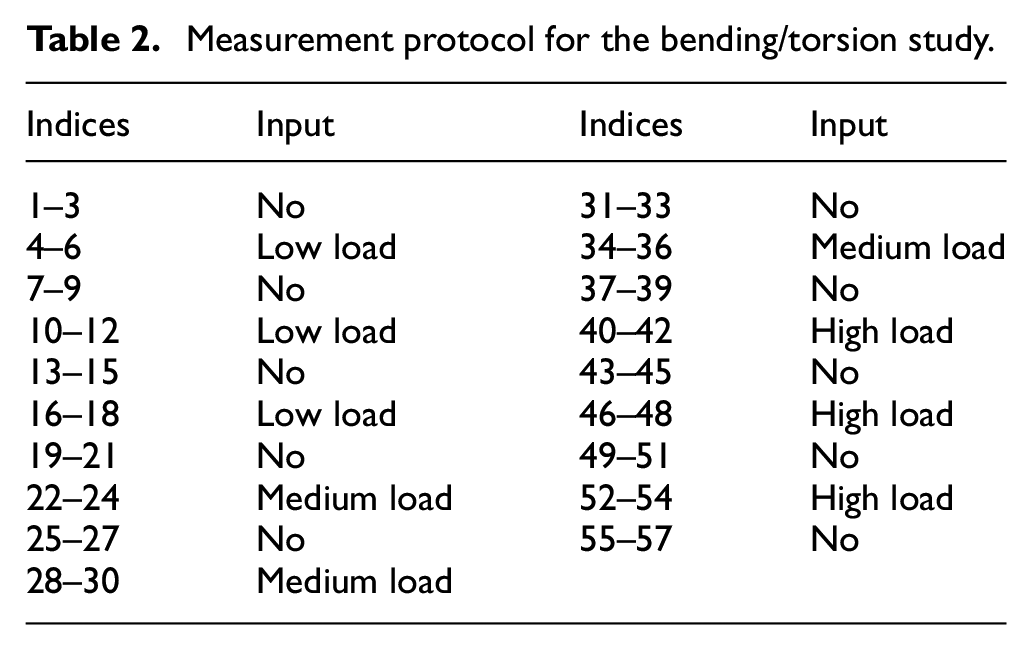
For the joint bending-and-torsion experiments, the demonstrator rudder stock with reduced size and a total length of 2627 mm is shown on the right-hand side of Figure 4. Again, the maximal diameter is 206 mm and also a material mixture of steel/CFRP is used. Different load scenarios are considered with a load and torque of 192 kN/27 kNm (low load), 288 kN/40.5 kNm (medium load) as well as 384 kN/54 kNm (high load), respectively. The measurement protocol is given in Table 2. A total of $n = 57$ measurements have been carried out with three-fold repetitions of subsequent measurements for better in-sample statistics. The damage which is to be detected has not been artificially and extrinsically induced, but is naturally caused by a certain amount of load. The result is a plastic deformation of the metal yielding a gap between the CFRP part and the steel. The measurement devices and the inspected frequency range are similar to those described in the previous section.

Table 2.

Measurement protocol for the bending/torsion study.

Indices	Input	Indices	Input
1–3	No	31–33	No
4–6	Low load	34–36	Medium load
7–9	No	37–39	No
10–12	Low load	40–42	High load
13–15	No	43–45	No
16–18	Low load	46–48	High load
19–21	No	49–51	No
22–24	Medium load	52–54	High load
25–27	No	55–57	No
28–30	Medium load

4. Results and discussion

The measured data from the bending study has been presented previously (Moll et al., 2020a) and portions of the data from the combined bending/torsion experiments have also appeared as a recent conference contribution (Moll et al., 2020b). However, only the measurement results have been published, all other parts of the present work represent novel and original content. For the sake of coherence, in Figure 5 an interesting spectral region of the measured susceptance is reproduced. 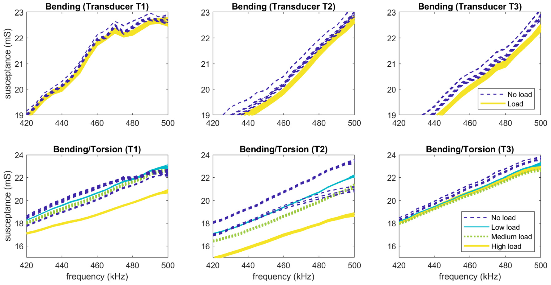The complete spectrum consists of $m = 96$ equidistant frequency points from 25 to 500 kHz. In the next section, the automatic, data-driven separation of the depicted bunches of similar curves into clusters is discussed.

Figure 5.

Spectra from the bending (top row) and the bending/torsion study (bottom) for transducer T1 (left column) to T3 (right). The high frequencies are depicted where the influence of applied loads is easily visible. Each line represents one measurement and is colored according to the distinct loads. Measurements with no load appear as two bunches due to the pristine or damaged state.

4.1. Automatic optimal dissimilarity-type clustering

So as to understand in a first step the measurements independent of the their annotations (e.g. pristine, load, damage), the all-to-all distances between the spectra are evaluated and shown in Figure 6. The all-to-all dissimilarity matrices are an continuation and also extension of the DI-based perspective (Moll et al., 2020a, 2020b) where merely the distance to the initial baseline measurements has been taken into account.

Figure 6.

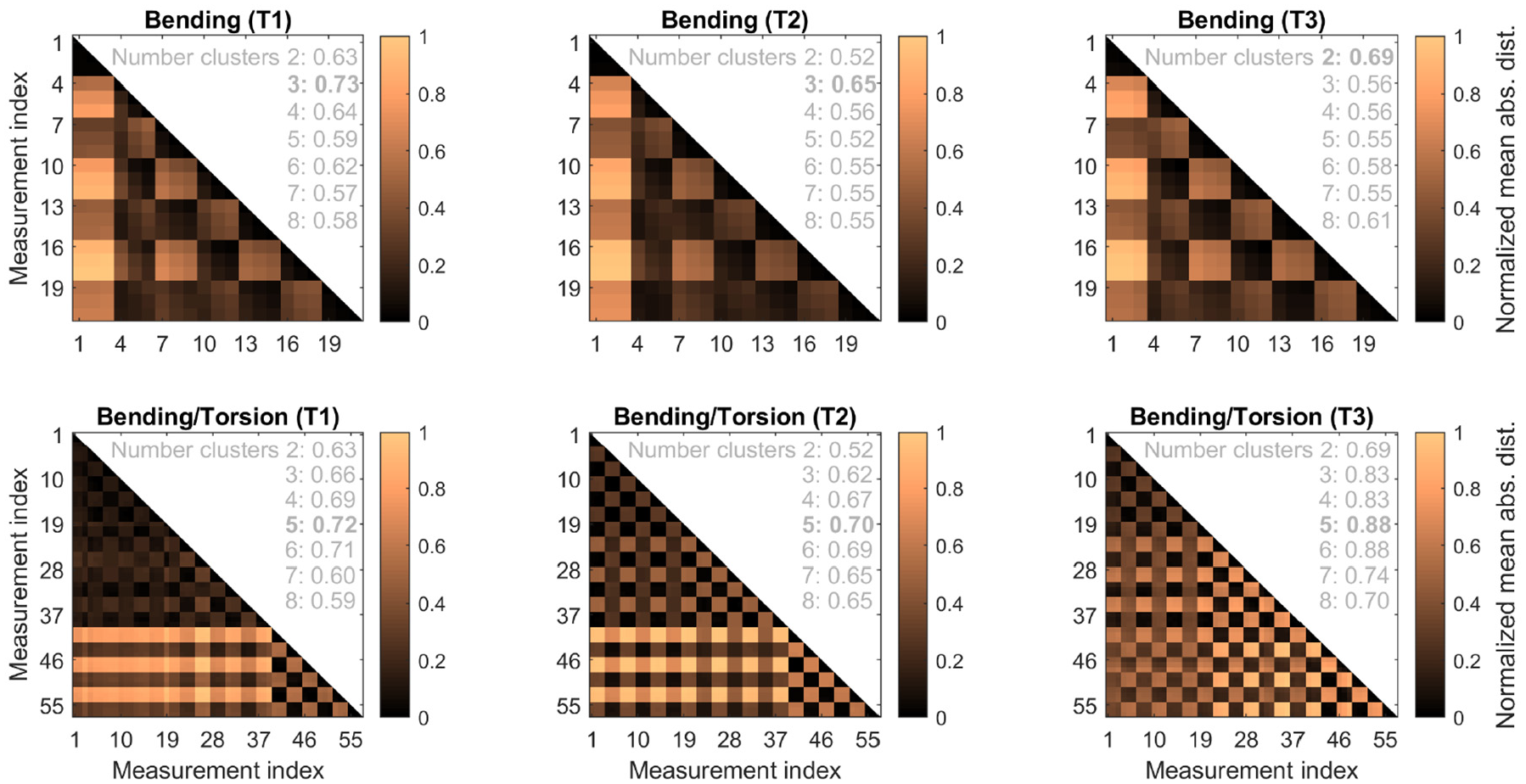
Pairwise dissimilarity of spectra from the bending (top row) and the bending/torsion study (bottom) for transducer T1 (left) to T3 (right). For every measurement pair the absolute distance is averaged across all frequencies and normalized in order to arrive at a maximum MAD of 1. Using Ward’s hierarchical clustering, as inset in gray font the Silhouette coefficients are written for potential cluster numbers. The optimal number of clusters $\tilde{N}$ is printed bold. Two out of the three transducers give rise to an optimal cluster number of $\tilde{N} = 3$ . For the combined bending/torsion study, all transducers indicate $\tilde{N} = 5$ .

Given the distance matrix, for each transducer a natural clustering is automatically sought using the silhouette coefficient $S$ defined in equation (6). For the bending study, the majority of transducers suggest data-driven an optimal cluster number of $\tilde{N} = 3$ . For the combined bending/torsion study, all the transducers suggest an optimal cluster number of $\tilde{N} = 5$ . When accepting the majority vote on the number of clusters, the assignment of an individual measurement to one of the clusters can be examined: In Figure 7 the memberships of the susceptance measurement belonging to the different clusters are depicted. For the bending study (left plot) the clusters are dubbed A to C whereas for the joint bending/torsion study (right plot) the clusters are dubbed D to H. Here, cluster label B should not be confused with susceptance $B$ or the susceptance data matrix $B$ . On a few points the membership is ambiguous: For measurement index 4 in the binding study and for the indices 40–42 in the combined bending/torsion study, the assignment is inconsistent across the three transducers. Based on the previous works (Moll et al., 2020a, 2020b), it becomes evident that the inconsistent membership assignment arises for those measurement indices, that is, those points in time, where a damaging of the rudder stocks happens. Since those measurement indices, that is, those instants of time, are especially critical for defect detection, the ambiguities call for further analysis.

Figure 7.

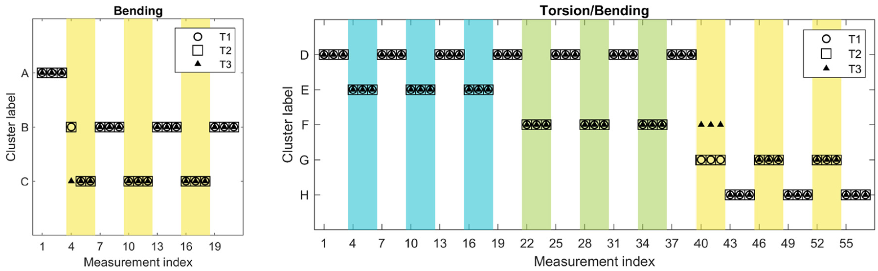
Clustering of the measurements for the bending study (left plot) and for the joint bending/torsion study (right plot) into 3 and 5 clusters, respectively, using Ward’s method. The pristine state with no load is named A for the bending study (left plot) and named D for the joint bending/torsion study (right plot). Measurements with load are indicated in the plots with a colored background area.

4.2. Principal component feature space analysis

The analysis of principal components allows for a complementary explorative look on the measurement data by explicitly embedding the measurement points into the feature space which is spanned by the principal components. In Figure 8 the decomposition into principle components is provided for the bending study. The two components which are determined through SVD and which are given in the upper row of Figure 8 for each transducer are in fact similar to what is expected from the theoretical considerations concerning the stylized susceptance spectra in Figure 5. The two components are on the one hand a roughly linear trend line and on the other hand an oscillatory residual component.

Figure 8.

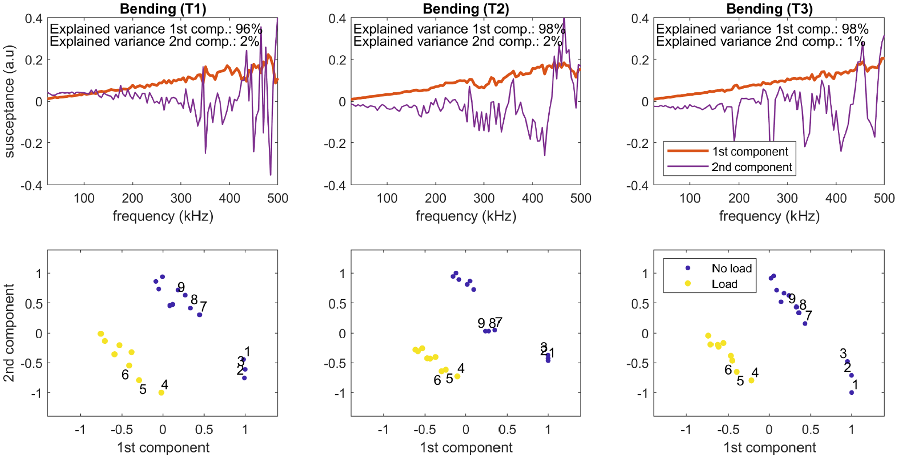
Principal components (top row) and the scores of each measurement along the two components (bottom row) for transducer T1 (left column), T2 (middle), and T3 (right) in the bending study. For orientation some measurements indices are given and each point is colored according to the presence or absence of load. The measurements indices are detailed in Table 1.

In the lower row of Figure 8 a clear distinction is possible between the pristine, loaded and unloaded but damaged state. For transducer T2 the measurements 7–9 appear as separate cluster indicating an intermediate state between pristine and damaged. This evidence has not be observed otherwise. Furthermore, in the feature space spanned by the two principal components, measurement 4 indeed lies at the fringe of its cluster (for all three transducers). For measurement index 4 there has been an ambiguous membership assignment regarding the dissimilarity-based clustering on the left plot in Figure 7. The feature space and the overall distribution of the measurements in the feature space are remarkably coherent across all three transducers.

For the combined bending/torsion study, the decomposition is depicted in Figure 9. In contrast to the bending study stands that the locations of the clusters are not coherent when comparing T1, T2, and T3. However, what the measurement data decompositions have in common across all the transducers is that indeed 5 well-defined clusters are visible. For transducer T3 nevertheless the measurements with indices 40–42 form a slightly pronounced sub-cluster which might be related to the previously discussed inconsistent assignment and might be again an intermediate state between intact and damaged.

Figure 9.

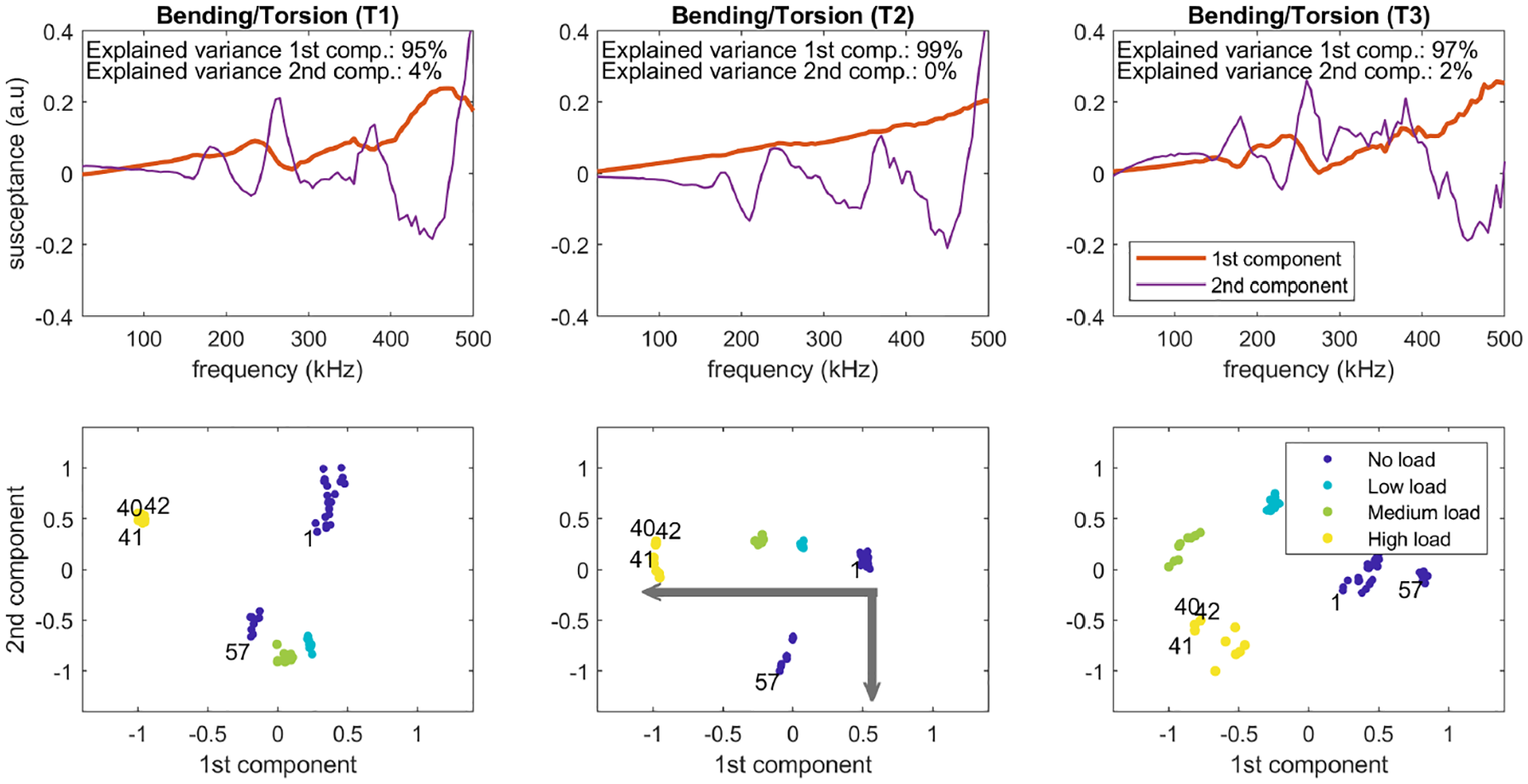
Principal components (top row) and the scores of each measurement along the two components (bottom row) for transducer T1 (left column), T2 (middle), and T3 (right) in the joint bending/torsion study. For orientation some measurements indices are given and each point is colored according to the distinct loads. The measurements indices are detailed in Table 2.

Remarkably, for T2 the different load states lie in one direction along the first component and discrimination between unloaded pristine versus unloaded damaged is mostly associated with the second component. The two gray arrows should help to guide the eye and underline this finding in the middle plot of the lower row in Figure 9.

4.3. Dynamic frequency-warping damage indicator

Principal component analysis and SVD rely on a more extensive history of measurements. This stands in contrast to the common approach of a DI tied to a few baseline measurements only. Nonetheless, the insights gained from SVD enable the improvement of the common DI-based approach: From the middle column of Figure 9, it has become clear that for a suitable sensor configuration, that is, transducer T2, SVD yields an approximately linear first component and a somewhat more complicated second residual component. Here, the first component replicates variations in slope due to load. In the Section “Methodology,” dynamic warping has been introduced which can potentially mitigate the effect of load on the spectrum. The dynamic distance thus quantifies the remaining residual contribution, that is, damage, which could not be compensated for in the alignment of the spectra.

The following comparative analysis has been carried out: (i) Warping is compared to the conventional DI approach using a static distance and (ii) at the same time a reduction of the necessary frequency points per spectrum is examined. Because warping delivers the most meaningful results when an equidistant sampling of the sequences is observed, in the analysis an equidistant spacing between frequency points is considered accordingly. The distance, also dubbed DI here, of the loaded state relative to a baseline as well as the distance of the state with damage (no load applied) relative to baseline are evaluate. If the DI for the loaded state is smaller than the DI for the damaged state than a true positive detection is counted. All 1701 possible spectra combinations are compared: nine under medium load, nine damaged with no load, and 21 baselines (see Table 2 for a list of conducted measurements).

In Figure 10 the results of the comparison is provided. For T1, both approaches work similarly well, for T3 they work similarly poor, however for T2 a significantly improved damage detection can be seen if the dynamic distance is employed as DI. The results in Figure 10 have been obtained by using solely $m^{*} = 10$ equidistant frequency points, that is, from 40 to 490 kHz, instead of $m = 96$ . In Figure 11 the exemplary susceptance spectra are given after warping: Since frequency warping performs a pairwise alignment, each exemplary spectrum is given with its warped baseline. The two examples in each plot are the damaged state without load and the pristine state with medium load. Their distance is evaluated relative to a baseline, that is, a state with no load and no damage. In Figure 11, for T1 and T2 the distance between warped baseline and warped spectrum under load is smaller than the distance between corresponding warped baseline and the warped spectrum in the presence of damage. For T3, warping in combination with the transducer’s configuration, that is, position and its bonding and the exact procedure of its attachment as well as other factors, does not lead to an enhance damage detection. Here, further research is needed to shed light on the contributing factors in greater detail.

Figure 10.

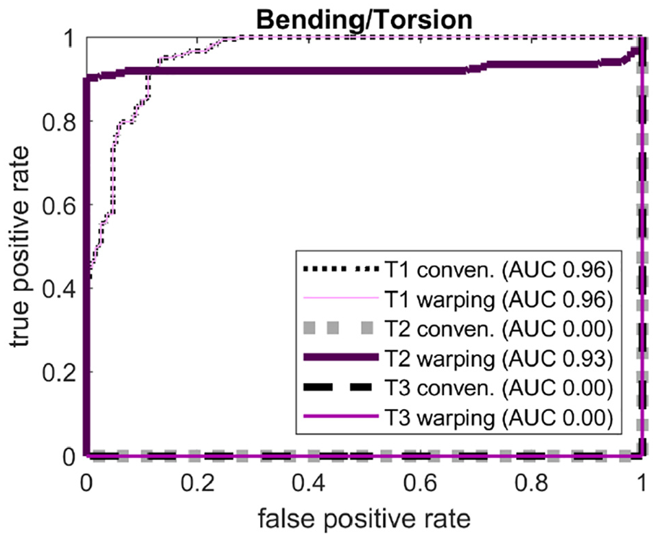
Comparison of the DI relying on the dynamic-warping MAD and the conventional MAD relative to a baseline (both for the joint bending/torsion study). The comparison is formulated as a binary classification task discriminating between the damaged state without load and the pristine state with medium load. The comparison is based on ROC curves and as a figure-of-merit the corresponding AUC is also provided. For T2 frequency warping significantly improves damage detection whereas the configuration of T3 seems not to allow for an improvement.

Figure 11.

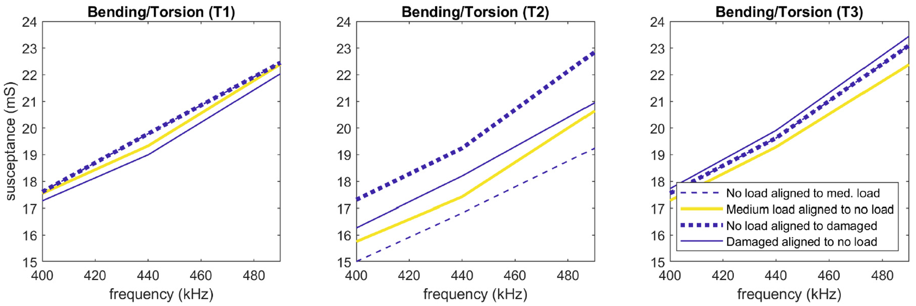
Exemplary susceptance spectra after warping (from the joint bending/torsion study) for transducer T1 (left column), T2 (middle), and T3 (right). The high-frequency portion of the spectrum is depicted where deviations between the warped spectra (loaded or damaged) to their respective warped baseline is visible. Details are provided in the text.

4.4. Tree classifiers for semi-supervised learning

The unsupervised decomposition has helped to enhance the DI-related SHM task of damage detection. This presented unsupervised processing can furthermore be seen as a first step for identifying annotations (or cluster labels) of the measurement data. In the combined bending/torsion study, each measurement has been assigned to a distinct cluster. After this unsupervised learning step, a supervised model, for example, a tree classifier, can be trained for correctly classifying freshly incoming measurements as damage or pristine even in the presence of load. Therefore, for every transducer a tree classifier has been trained taking the susceptance spectra as input with the label as response variable. Besides just learning the data, trees are able to identify the most important predictors, that is, frequency points in the susceptance spectrum. It has been possible to select as few as two features (or frequencies) that are shared across all transducers and that can separate pristine and damage states in the feature space. At most three splits regarding those to features are needed. The results of training classification trees are plotted in Figure 12. The most complex tree, that is, for T2, is drawn in Figure 1.

Figure 12.

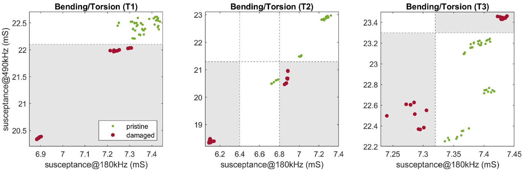
Decision boundaries of the tree classifier discriminating between damaged and pristine states for transducer T1 (left column), T2 (middle), and T3 (right) in the joint bending/torsion study. Measurements are plotted in a two-dimensional feature space. These two important features (or predictors or variables) result from training the classification trees and therewith evaluating feature importance. Among the 96 frequency points, the combination of for example, these two features is critical from damage detection.

5. Conclusions

Two innovative rudder stocks have been investigated using the EMI method. In particular, two different multi-sensor data sets of experimental measurements have been analyzed with a range of statistical processing approaches. The focus has been on the detection of damage in the obstructive presence of external load. Backed by theoretical consideration about the influence of EOC on EMI spectra, an improved DI has been introduced based on dynamic frequency warping. Given a suitable sensor configuration, dynamic frequency warping facilitates the compensation of load. Furthermore, unsupervised machine learning, that is, cluster analysis, and supervised machine learning, that is, classification trees, have been combined in order to…

… reveal undiscovered patterns in the data sets, such as intermediate structural states between intact and damaged.

… automatically generate class labels that can subsequently be learned by a classifier.

… facilitate damage detection even under load.

… identify the most important parts of the spectrum and therefore help to reduce the number of needed frequency points.

… achieve damage detection using simple rules encoded in a decision tree which can be run on low-cost, low-power SHM devices.

Because the discussed methodology is quite general as well as likely applicable beyond EMI and beyond the presented use case for the maritim industies, future research aims at deploying it to a wider range of problems.

Footnotes

Acknowledgements

The authors thank Matthias Schmidt and Johannes Käsgen (Fraunhofer LBF) as well as Jörg Mehldau (Becker Marine Systems), Marcel Bücker (Institut für Verbundwerkstoffe), Felix Haupt (CCOR-Schäfer MWN) for their help in compiling the measurement data.

Declaration of conflicting interests

The authors declared no potential conflicts of interest with respect to the research, authorship, and/or publication of this article.

Funding

The authors disclosed receipt of the following financial support for the research, authorship, and/or publication of this article: The authors acknowledge financial support of this research by the German Federal Ministry for Economic Affairs and Energy under grant 03SX422A-D. Additional financial support is provided by the German Federal Ministry of Education and Research under grant 13GW0502B.

ORCID iDs

Christian Kexel

Jochen Moll

References

Annamdas

VGM

Soh

(2010) Application of electromechanical impedance technique for engineering structures: Review and future issues. Journal of Intelligent Material Systems and Structures 21(1): 41–59.

Bergmann

Fauser

Sattlegger

, et al. (2019) MVTec AD–a comprehensive real-world dataset for unsupervised anomaly detection. In: Proceedings of the IEEE/CVF conference on computer vision and pattern recognition, Long Beach, CA, 15–20 June 2019, pp.9592–9600. New York: IEEE.

Bosse

Lehmhus

Lang

, et al. (2018) Material-Integrated Intelligent Systems: Technology and Applications. Weinheim: John Wiley & Sons.

Croxford

Moll

Wilcox

, et al. (2010) Efficient temperature compensation strategies for guided wave structural health monitoring. Ultrasonics 50(4–5): 517–528.

Deng

Dong

Socher

, et al. (2009) Imagenet: A large-scale hierarchical image database. In: 2009 IEEE conference on computer vision and pattern recognition, Miami, FL, 20–25 June 2009, pp. 248–255. New York: IEEE.

Douglass

Harley

(2020) Model-based statistical guided wave damage detection for an aluminum plate. Structural Health Monitoring 19(6): 1937–1950.

Douglass

ACS

Harley

(2018) Dynamic time warping temperature compensation for guided wave structural health monitoring. IEEE Transactions on Ultrasonics Ferroelectrics and Frequency Control 65(5): 851–861.

Efron

Hastie

(2016) Computer Age Statistical Inference, vol. 5. New York, NY: Cambridge University Press.

Fritzen

Kraemer

(2009) Self-diagnosis of smart structures based on dynamical properties. Mechanical Systems and Signal Processing 23(6): 1830–1845.

10.

Giurgiutiu

(2014) Structural Health Monitoring: With Piezoelectric Wafer Active Sensors. Amsterdam: Academic Press.

11.

Hage

Heredia Conde

Loffeld

(2020) Sparse signal recovery via kalman-filter-based ℓ1 minimization. Signal Processing 171: 107487.

12.

Hastie

Tibshirani

Friedman

(2009) The Elements of Statistical Learning: Data Mining, Inference, and Prediction. New York: Springer Science & Business Media.

13.

Hastie

Tibshirani

Wainwright

(2015) Statistical Learning With Sparsity: The Lasso and Generalizations. Boca Raton: Chapman and Hall/CRC.

14.

Jung

Park

, et al. (2014) Relative baseline features for impedance-based structural health monitoring. Journal of Intelligent Material Systems and Structures 25(18): 2294–2304.

15.

Kaur

Bhalla

Maddu

(2019) Damage and retrofitting monitoring in reinforced concrete structures along with long-term strength and fatigue monitoring using embedded lead zirconate titanate patches. Journal of Intelligent Material Systems and Structures 30(1): 100–115.

16.

Kaur

Bhalla

, et al. (2017) Integration and evaluation of multiple piezo configurations for optimal health monitoring of reinforced concrete structures. Journal of Intelligent Material Systems and Structures 28(19): 2717–2736.

17.

Kexel

Maetz

Mälzer

, et al. (2021) Ultrasonic data transmission across metal structures affected by environmental conditions. Journal of Sound and Vibration 490: 115691.

18.

Kexel

Testoni

Zonzini

, et al. (2020) Low-power mimo guided-wave communication. IEEE Access 8: 217425–217436.

19.

Lammering

Gabbert

Sinapius

, et al. (2017) Lamb-Wave Based Structural Health Monitoring in Polymer Composites. Berlin: Springer.

20.

Lim

Smith

Padilla

, et al. (2021) Monitoring of concrete curing using the electromechanical impedance technique: Review and path forward. Structural Health Monitoring 20(2): 604–636.

21.

Lin

Maire

Belongie

, et al. (2014) Microsoft coco: Common objects in context. In: European conference on computer vision. Zurich, Switzerland, 6–12 September 2014, pp. 740–755. New York: Springer.

22.

Loh

(2011) Classification and regression trees. WIREs Data Mining and Knowledge Discovery 1(1): 14–23.

23.

Loh

(2002) Regression tress with unbiased variable selection and interaction detection. Statistica Sinica 12(2): 361–386.

24.

Madhav

AVG

(2007) Characterization of smart PZT transducer and admittance signatures using PZT-structure interaction models for structural health monitoring. PhD Thesis, Nanyang Technological University, Singapore.

25.

Memmolo

Monaco

Boffa

, et al. (2018) Guided wave propagation and scattering for structural health monitoring of stiffened composites. Composite Structures 184: 568–580.

26.

Migot

Mei

Giurgiutiu

(2021) Numerical and experimental investigation of delaminations in a unidirectional composite plate using ndt and shm techniques. Journal of Intelligent Material Systems and Structures 32: 1781–1799.

27.

Moll

(2019) Damage detection in grouted connections using electromechanical impedance spectroscopy. Proceedings of the Institution of Mechanical Engineers Part C Journal of Mechanical Engineering Science 233(3): 947–950.

28.

Moll

Kexel

Milanchian

, et al. (2019a) Ultrasound bone fracture sensing and data communication: Experimental results in a pig limb sample. Ultrasound in Medicine & Biology 45(2): 605–611.

29.

Moll

Kexel

Pötzsch

, et al. (2019b) Temperature affected guided wave propagation in a composite plate complementing the open guided waves platform. Scientific Data 6(1): 191.

30.

Moll

Schmidt

Käsgen

, et al. (2020a) Detection of pin failure in carbon fiber composites using the electro-mechanical impedance method. Sensors 20(13): 3732.

31.

Moll

Schmidt

Käsgen

, et al. (2020b) Load and structural health monitoring of a scaled cfrp rudder stock using electro-mechanical impedance technique. In: Fromme

(ed.) Health Monitoring of Structural and Biological Systems XIV, vol. 11381. International Society for Optics and Photonics. p.1138135.

32.

Mueller

(2017) Inspection of piezoelectric transducers used for structural health monitoring systems. PhD Thesis, University of Siegen, Germany.

33.

Mueller

Fritzen

(2017) Inspection of piezoceramic transducers used for structural health monitoring. Materials 10(1): 71.

34.

Needleman

Wunsch

(1970) A general method applicable to the search for similarities in the amino acid sequence of two proteins. Journal of Molecular Biology 48(3): 443–453.

35.

Neubeck

Kexel

Moll

(2020) Matrix techniques for lamb-wave damage imaging in metal plates. Smart Materials and Structures 29(11): 117003.

36.

Neuburg

(1988) Frequency warping by dynamic programming. In: ICASSP-88., international conference on acoustics, speech, and signal processing, New York, NY, 11–14 April 1988, pp. 573–574. New York: IEEE Computer Society.

37.

Neuschwander

Moll

Memmolo

, et al. (2019) Simultaneous load and structural monitoring of a carbon fiber rudder stock: Experimental results from a quasi-static tensile test. Journal of Intelligent Material Systems and Structures 30(2): 272–282.

38.

Overly

TGS

Park

Farinholt

, et al. (2008) Development of an extremely compact impedance-based wireless sensing device. Smart Materials and Structures 17(6): 065011.

39.

Park

Lee

Yun

, et al. (2008) Electro-mechanical impedance-based wireless structural health monitoring using PCA-data compression and k-means clustering algorithms. Journal of Intelligent Material Systems and Structures 19(4): 509–520.

40.

Rautela

Senthilnath

Moll

, et al. (2021) Combined two-level damage identification strategy using ultrasonic guided waves and physical knowledge assisted machine learning. Ultrasonics 115: 106451.

41.

Romesburg

(2004) Cluster Analysis for Researchers. Morrisville, NC: Lulu Press.

42.

Salas

Hubner

Borysov

, et al. (2018) Measuring material moisture in fiber reinforced polymers by integrated sensors. IEEE Sensors Journal 18(9): 3836–3843.

43.

Salehi

Burgueño

Chakrabartty

, et al. (2021) A comprehensive review of self-powered sensors in civil infrastructure: State-of-the-art and future research trends. Engineering Structures 234: 111963.

44.

Sheikhpour

Sarram

Gharaghani

, et al. (2017) A survey on semi-supervised feature selection methods. Pattern Recognition 64: 141–158.

45.

Soman

Singh

Wandowski

, et al. (2020) Development of robust metric based on cumulative electrical power for electromechanical impedance based structural health monitoring. Smart Materials and Structures 29(11): 115047.

46.

Srivastava

Bhalla

Madan

(2017) Assessment of human bones encompassing physiological decay and damage using piezo sensors in non-bonded configuration. Journal of Intelligent Material Systems and Structures 28(14): 1977–1992.

47.

Tang

Yang

Soh

(2010) Toward broadband vibration-based energy harvesting. Journal of Intelligent Material Systems and Structures 21(18): 1867–1897.

48.

Tekkalmaz

Haydarlar

Sofuoğlu

(2020) A statistical analysis of temperature compensation for piezoelectric sensor bonded to aisi-1080 material. Proceedings of the Institution of Mechanical Engineers Part C Journal of Mechanical Engineering Science. Epub ahead of print 16 December 2020. DOI: 10.1177/0954406220978250.

49.

Tenreiro

AFG

Lopes

da Silva

(2021) A review of structural health monitoring of bonded structures using electromechanical impedance spectroscopy. Structural Health Monitoring. Epub ahead of print 17 March 2021. DOI: 10.1177/1475921721993419.

50.

Toda

Saruwatari

Shikano

(2001) Voice conversion algorithm based on Gaussian mixture model with dynamic frequency warping of STRAIGHT spectrum. In: 2001 IEEE international conference on acoustics, speech, and signal processing. Proceedings (Cat. No. 01CH37221) (ed Mathews

), vol. 2, Salt Lake City, Utah, USA, 7–11 May 2001, pp.841–844. New York: IEEE.

51.

Wandowski

Malinowski

Ostachowicz

(2017) Temperature and damage influence on electromechanical impedance method used for carbon fibre–reinforced polymer panels. Journal of Intelligent Material Systems and Structures 28(6): 782–798.

52.

Ward

Jr (1963) Hierarchical grouping to optimize an objective function. Journal of the American Statistical Association 58(301): 236–244.

53.

Zonzini

Zauli

Mangia

, et al. (2021) Model-assisted compressed sensing for vibration-based structural health monitoring. IEEE Transactions on Industrial Informatics 17: 7338–7347.

Detecting damage in rudder stocks under load using electro-mechanical susceptance: Frequency-warping and semi-supervised approaches

Abstract

Keywords

1. Introduction

2. Methodology

2.1. Binary classification and classification trees

2.2. Principal components and cluster analysis

2.3. Dynamic frequency warping compensation

2.4. Electro-mechanical impedance spectroscopy

3. Setup

3.1. Bending study

3.2. Combined bending/torsion study

4. Results and discussion

4.1. Automatic optimal dissimilarity-type clustering

4.2. Principal component feature space analysis

4.3. Dynamic frequency-warping damage indicator

4.4. Tree classifiers for semi-supervised learning

5. Conclusions

Footnotes

Acknowledgements

Declaration of conflicting interests

Funding

ORCID iDs

References