Sage Journals: Discover world-class research

Abstract

We consider income-source-dependent tax evasion and show that this is a generalisation of the well-known endowment effect. We show that loss aversion, moral costs, mental accounting and risk preferences play a role in explaining key features of source-dependent tax evasion. We provide evidence of the first direct link between subject-specific loss aversion and tax evasion, which is central to most successful modern theoretical accounts of tax evasion. We provide some evidence that risk aversion strengthens the cautionary effect of loss aversion and risk loving behaviour attenuates, or reverses, it. However, the underlying effect is also influenced by the source of income. Evasion is increasing in the tax rate and decreasing in the audit penalty, as predicted. Our study provides novel theoretical insights; proposes new methods in the estimation of the underlying behavioural parameters; and confirms the central predictions of the theory, while pointing out challenges for further developments that existing theory is unable to account for.

JEL: C91, C92, D82, D91, G21

Keywords

Tax evasion endowment effect loss aversion morality mental accounting prospect theory risk aversion

I Introduction

Tax evasion is an important area of research within public economics with significant welfare consequences.¹ This problem has attracted a great dea of academic interest.² The Allingham-Sandmo (1972) model established the basic framework, based on expected utility, but the empirical success of this framework has been questionable, giving rise to the well-known tax evasion puzzles. The puzzles are both quantitative³ and qualitative⁴ By contrast, non-expected utility theories such as prospect theory provide a better explanation of the tax evasion evidence (Bernasconi, 1998; Yaniv, 1999; Bernasconi & Zanardi, 2004; Dhami & al-Nowaihi, 2007, 2010; Eide et al., 2011).⁵

Loss Aversion and Tax Evasion

The key features in the success of prospect theory in explaining the qualitative and quantitative puzzles in tax evasion are reference dependence and loss aversion. This is true of the theoretical models (Bernasconi, 1998; Yaniv, 1999; Bernasconi & Zanardi, 2004; Dhami & al-Nowaihi, 2007, 2010; Eide et al., 2011; Alm & Torgler, 2012) and of empirical studies that use data from field observational studies (Engström et al., 2015; Rees-Jones, 2018). Loss aversion also influences much human and primate behaviour and is also well supported by neuroeconomic evidence (Dhami, 2019, Vol. 1).

Despite the key importance of loss aversion, we are not aware of empirical work that rigorously and directly measures loss aversion for 'individual' taxpayers and relates it to their tax evasion behaviour.⁶ Observational studies and studies based on administrative data attempt to study indirect implications of reference dependence and loss aversion, such as bunching of taxpayers where there are kinks in the marginal tax/subsidy rates. Direct measurement of loss aversion at the level of each taxpayer is a specialised, complex and time consuming, task and requires measurement of all parameters of prospect theory in one fell swoop.⁷

The 'main aim' of our study is to provide a direct examination of the underlying mechanisms of prospect theory-based explanations of tax evasion, by directly measuring individual-specific loss aversion in lab experiments. We then relate individual-specific loss aversion with the tax evasion decisions of the same individual.

Source-Dependent Evasion

Extensive evidence shows that humans experience different levels of entitlements from earned and unearned incomes.⁸ In the classic endowment effect studies, entitlements are themselves caused by loss aversion (Kahneman & Tversky, 2000; Dhami, 2019, Vol. 1). We wish to examine the income-source-dependence of tax evasion (source dependent evasion) when the different income sources are identical in their tax/deterrence treatment. In particular, we compare labour income, earned in a tedious experimental task, relative to non-labour income which is unearned during the experiment, for example, bequests, gifts, lottery wins, unexpected capital gains. Our proposed theory allows for potentially any difference in the two income sources, provided the individual feels more entitled to one income source over the other.

If taxpayers evade different amounts from the two different sources of incomes, then this may also indicate a form of mental accounting. Thaler (1999, p. 186) gave a general definition of mental accounting: 'I wish to use the term 'mental accounting' to describe the entire process of coding, categorizing, and evaluating events'.⁹ Source-dependent tax evasion behaviour, if confirmed, potentially indicates mental accounting because tax evaders then appear to code and categorise different income sources, identical in their tax/deterrence treatment, differently.¹⁰

It is an interesting research question to see if there is any interaction between the source of income, loss aversion and risk aversion. This is the second objective of our study.

Following the earlier literature, cited above, we hypothesise that people feel more entitled to (earned) labour income relative to (unearned) non-labour income. We conjecture two effects, working in opposite directions, through which entitlements to income might influence tax evasion. (i) First, loss aversion arising from being caught evading taxes is greater from income that one feels more entitled to (earned income) relative to unearned income, and our data supports it. Our theoretical model shows that higher loss aversion reduces evasion. Hence, individuals should evade less earned income as compared to unearned income. (ii) Second, we hypothesise that there are lower moral cost from evading earned labour income. In some sense, individuals feel less guilty from evading income they are more entitled to. Our theoretical model predicts that lower moral costs from evasion will result in more evasion of labour income. There is no satisfactory method of directly measuring income source-specific moral costs for each taxpayer, but we provide indirect evidence, consistent with moral costs.¹¹

From (i) and (ii) above, greater loss aversion reduces evasion and lower moral costs increase evasion of earned income. Thus, the overall treatment effect, which determines the relative tax evasion from labour and non-labour income, is an empirical question.¹² We note that, nevertheless, a predicted ambiguous result is also an important theoretical result that needed to be demonstrated rigorously. Furthermore, the sign of the treatment effects, based on our empirical analysis, speaks to the relative strengths of the two opposite effects.

Loss Aversion and Risk Aversion

Traditional analyses of risky situations, based on expected utility theory, highlight the importance of risk aversion in explaining individual choices.¹³ By contrast loss aversion is a property of the utility function under prospect theory, not related to its curvature, and it arises in riskless choices as well as risky choices. Risk aversion and loss aversion are distinct, yet related, entities in prospect theory.¹⁴

There are claims that once loss aversion is accounted for, there is 'no' remaining risk aversion (Novemsky & Kahneman, 2005). In other words, the claim is that observed risk aversion is likely to be mostly on account of loss aversion, but unless one separately measures them, results may be confounded. There is no simple relation between risk aversion and loss aversion under prospect theory if there are outcomes in, both, the domains of gains and losses. However, we measure risk aversion in lotteries that are only in the domain of gains, while loss aversion is measured with both gain and loss lotteries; this removes the confounding role of loss aversion.

A third aim of our study is to measure risk aversion for each individual taxpayer and relate it to evasion behaviour, while also considering the interactions between risk aversion and loss aversion.

Theoretical Model

We use the framework in Dhami & al-Nowaihi (2007, 2010) to derive the implications of loss aversion and income-source dependence of tax evasion, using prospect theory. Since these results follow in a straightforward manner from their model, we relegate the detailed model to the supplementary section, and only list the two main propositions in the text as a guide to the predictions of the relevant model.

Experiments and Findings

We ran a between-subjects experiment over Zoom with Indian University students. Subjects are randomly assigned to either a primed or an unprimed group. The primed group is shown data about tax evasion in India. Within each group, subjects are assigned to two treatments. In the first treatment (T1), taxpayers have only non-labour, experimenter-provided, unearned income. In the second treatment (T2), the only source of income for taxpayers is labour income, earned by solving a set of timed and tedious experimental tasks. We control for taxpayer-specific preference characteristics (e.g. loss aversion, risk attitudes), economic characteristics (e.g. education) and demographic characteristics (e.g. age, gender, marital status, religion). In addition, we explore the effects of varying the tax and detection/enforcement parameters on tax evasion.¹⁵

Several empirical results support the predictions of our theoretical model. In the simplest estimation, under a linear utility function, the mean loss aversion for our data is 1.83. For a non-linear utility function, the mean loss aversion is 1.37 for non-labour income and 1.53 for labour income. This supports our conjecture on source dependent loss aversion.

Even when there is an effective 100% subsidy to evasion, taxpayers declare, on average, 35% of their income, which is consistent with the presence of moral costs of evasion.¹⁶ Moreover, in the presence of a subsidy to evasion, unprimed subjects declare, on average, more of their non-labour income, which is consistent with our hypotheses on income-specific differences. However, we do not measure moral costs for different sources of income, and it is not clear how to do so.¹⁷

In terms of 'direct effects' in a Tobit regression, those who are loss averse declare 18.1% more of their income, relative to those who are loss seeking. This is consistent with our theory. It also provides the first direct empirical evidence, using subject-specific, directly measured, loss aversion, for the underlying transmission channel in most 'prospect theory-based' explanations of tax evasion, as described above.

We also show that the effects of loss aversion are more complicated than anticipated. They are influenced by the source of income (as postulated), but also by risk preferences, in a manner which is a new result that cannot be accommodated within the predictions of our theoretical model, or any other decision theory model that we are aware of. Loss averse and risk averse taxpayers declare 7.6% more labour income relative to non-labour income. However, loss averse and risk loving subjects declare 19.3% less labour income, relative to non-labour income. It is 'as if' risk loving behaviour reverses the cautionary effects of loss aversion on declared incomes for labour income. Loss seeking and risk averse subjects declare 3.6% more labour income as compared to non-labour income. In this case, the cautionary effects of risk aversion seem to overweight the effects arising from loss seeking behaviour. However, this is not a general finding, as we also report exceptions depending on the source of incomes.

In conjunction, our results show that tax evasion behaviour is driven not just by loss aversion, but also by moral costs, mental accounting and risk preferences.

Finally, we confirm some of the standard effects that have already been identified or tested in other models. Our model predicts that tax evasion is decreasing in the deterrence parameters, audit probability and penalty rate, as in models based on expected utility theory, and we confirm this with our data. We also show that evasion is decreasing in the tax rate, as predicted by prospect theory, where no Yitzhaki puzzle arises.

Schematic Outline of Paper

Section II presents our model and summarises the theoretical predictions. Section III outlines our theoretical approach to measuring loss aversion and risk attitudes. Section IV describes the experimental design. Section V provides the descriptive statistics for the model and the findings on loss aversion and risk attitudes. Section V tests our comparative static predictions of the amount evaded with respect to the audit penalty rate and the tax rate. Section VI gives a Tobit analysis of the proportion of declared income and highlights its determinants. Section VII concludes. We provide the details of all the theoretical results in the study and some additional statistical findings in a separate supplementary section.

II The Model

We use the generic Allingham-Sandmo-Yitzhaki model of tax evasion, adapted to prospect theory by Dhami & al-Nowaihi (2007). We relegate the full model and the derivations to the supplementary section.¹⁸ We summarise the essential features of the model in this section, and the theoretical predictions in the next section.

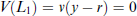
We distinguish between the source of the taxable income, that is either labour income, L, or non-labour income, N. We write the income of the taxpayer from source $j = L, N$ as $W_{j}$ . In our experiments, the taxpayer either has labour income $(j = L)$ or non-labour income $(j = N)$ , but never both. Hence, we may conserve notation further and dispense entirely with the subscript j and refer to the taxpayer as having unobserved taxable income W.

Each source of income is taxed at the identical constant marginal rate t, 0 < t < 1. The taxpayer chooses to declare income $D \in [0, W]$ and evades the amount W − D. The two deterrence parameters, audit probability, p, and the penalty rate, θ, are also identical for the two sources of incomes. Taxpayers are audited with the probability $p (D) \in [0, 1]$ , such that

\begin{matrix} p (D) = a - b D; a \in [0, 1], 0 \leq b \leq \frac{a}{W} . \end{matrix}

(1)

The restrictions on a,b ensure that $p (D) \in [0, 1]$ for all $D \in [0, W]$ . We term the case b = 0, so p(D) = a, as 'exogenous' audit probability; and the case b > 0 as 'endogenous' audit probability because it depends on declared income (an endogenous decision). An audit provides observable and verifiable information to the tax authorities on the true income, W. If caught, a tax evader must pay the outstanding tax liabilities t(W − D, and a penalty $θ t (W - D)$ , where θ is the penalty rate on evaded taxes. If θ < 0, then the government effectively subsidises tax evasion. In our experiments, we show that for θ = −1 (100% subsidy to the taxpayer if caught evading), there is significant declared income, which is consistent with underlying moral costs of evasion. However, our main case of interest is θ > 0. Thus, if caught, the taxpayer pays the following amount to the tax authorities

\begin{matrix} t (1 + θ) (W - D) \equiv t f (W - D), where f = 1 + θ . \end{matrix}

(2)

We call f the fine rate per unit of evaded taxes. A tax evader experiences morality costs $c \in [\underline{c}, \bar{c}]$ per unit of evaded taxes, irrespective of whether caught or not. We assume that (i) morality costs are non-negative ( $\underline{c} \geq 0$ ), and (ii) no higher than the tax rate.²⁰

We use prospect theory in our analysis. In prospect theory, taxpayers are either in the domain of gains (income greater than reference point) or in the domain of losses (income lower than the reference point). The 'status-quo' serves as a powerful reference point for humans, animals and plants (Kahneman & Tversky, 1979; Kahneman & Tversky, 2000; Dhami, 2019, Vol. 1). Furthermore, the legal framework (e.g. legal tax liabilities) provides a useful, and empirically satisfactory, reference point and enhances the status-quo in applications, particularly tax evasion (Dhami & al-Nowaihi, 2007, 2010).²¹ For this reason, we define the reference income, R, of the taxpayer to be the legal after-tax income

R = (1 - t) W .

Dhami & al-Nowaihi (2007) show that this is the 'unique' reference point such that for any level of declared income, $D \in [0, W]$ , the taxpayer is always in the domain of gains if not caught evading, and in the domain of losses if caught evading taxes.²² We use the standard prospect theory utility function (Kahneman & Tversky, 1979; Tversky & Kahneman, 1992), which has axiomatic foundations (al-Nowaihi et al., 2008):

\begin{matrix} v (x) = \{\begin{array}{l} {(x)}^{γ} & if x \geq 0 \\ - λ {(x)}^{γ} & if x < 0 \end{array}, \end{matrix}

(3)

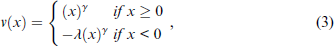
where x is an outcome relative to a reference point. The typical restriction on the two parameters in (3) are $0 < γ < 1$ and $λ > 1$ (loss aversion). But in our empirical exercise we also allow for $λ < 1$ (loss seeking).

As discussed in the introduction, earned labour income may create greater entitlements relative to unearned non-labour income through differences in loss aversion and moral costs of evasion. A formal statement of this assertion requires us to temporarily invoke the subscript $j = L, N$ for the source of income that was suppressed above. Let $c_{j}, λ_{j}$ denote, respectively, moral cost of evasion and loss aversion for the taxpayer from income source $j = L, N$ . Then, the taxpayer exhibits relatively lower moral cost of evading labour income to which the taxpayer feels more entitled to

\begin{matrix} c_{L} < c_{N}, \end{matrix}

(4)

and relatively higher loss aversion from labour income (giving up a unit of income that one feels more entitled to, is more aversive).

\begin{matrix} λ_{N} < λ_{L} . \end{matrix}

(5)

We allow for individual-specific and income-source-specific heterogeneity in preference parameters, but suppress it in the formal notation.

We now directly give the theoretical predictions of the model. The details of the derivations are in the supplementary section. There are two states of the world. (1) $s = C$ if the taxpayer is 'caught' evading taxes. (2) $s = N C$ if the taxpayer is 'not caught' evading taxes.

Proposition 1. Consider an interior solution to optimal declared income $D^{*} \in$ $(0, W)$ and an endogenous probability of detection $p (D) = a - b D, a \in [0, 1] b > 0.$ ²³

(a) (Effectiveness of deterrence) $D^{*}$ is increasing in the penalty rate, that is, $\frac{\partial D^{*}}{\partial θ} > 0$ , and in the probability of detection parameter, a, that is, $\frac{\partial D^{*}}{\partial a} > 0.$ ²⁴

(b) (Loss aversion) $D^{*}$ is increasing in the parameter of loss aversion, λ, that is, $\frac{\partial D^{*}}{\partial λ} > 0$ .

(c) (Explanation of Yitzhaki puzzle) $D^{*}$ is decreasing in the tax rate, that is, $\frac{\partial D^{*}}{\partial t} < 0$ .

(d) (Morality costs) $D^{*}$ is increasing in the morality costs from evasion, c, that is, $\frac{\partial D^{*}}{\partial c} > 0$ .

Discussion of the results: An increase in the probability of detection (the parameter 'a'), or an increase in the audit penalty, θ, reduces the expected marginal returns from evasion, which reduces evasion (Proposition 1a). An increase in loss aversion increases the losses that arise in the state $s = C$ , when caught evading taxes, reducing the marginal return from evasion, hence, reducing evasion (Proposition 1b). Prospect theory predicts that as the tax rate increases, evasion increases, in conformity with the available evidence, so there is no Yitzhaki puzzle under prospect theory (Proposition 1c).²⁵ This is a simple extension of the original result in Dhami & al-Nowaihi (2007). Finally, an increase in the moral cost, c, of tax evasion reduces evasion by reducing income relative to the reference point in both states of the world (Proposition 1d).

Recall from (4) and (5) our hypotheses that for earned labour income, loss aversion is relatively higher $(λ_{N} < λ_{L})$ and moral costs of evasion are relatively lower $(c_{L} < c_{N})$ . From Proposition 1 b an increase in loss aversion reduces evasion and from Proposition 1d, a reduction in moral costs increases evasion. Since these effects oppose each other, depending on the relative strengths of the two effects, the treatment effect (relative evasion in the two treatments) can be positive, zero or negative. Thus, the treatment effect is an entirely empirical question.

We now show how the result in Proposition 1 is modified with an exogenous probability of detection, $p (D) = a > 0$ (and $b = 0$ ), that is independent of the amount evaded; we consider this case in some of our experimental questions. In this case, we get a bang-bang solution in which the optimal declared income, $D^{*}$ , responds to critical values of the parameters and the policy parameters.

However, the intuition for the comparative static effects is as in Proposition 1, which we do not repeat here.

Proposition 2. Suppose that the probability of detection is exogenous, so that $p (D) = a > 0$ , for all $D \in [0, W]$ . Let $D^{*}$ be the optimal level of declared income.

(a) (Exogenous probability of detection, a) Let $a \in [0, 1]$ . Then there exists a critical value of $a = a_{c} > 0$ such that if $a < a_{c}, D^{*} = 0$ , and if $a > a_{c}$ , $D^{*} = W$ . When $a = a_{c}$ , we have $D^{*} \in [0, W]$ .

(b) (Penalty rate, θ) Let $θ \in [0, \overset{࿽}{θ}]$ , where $\overset{࿽}{θ}$ is the maximum possible penalty rate. Then there exists a critical value of $θ = θ_{c} > 0$ such that if $θ < θ_{c}$ , $D^{*} = 0$ , and if $θ > θ_{c}, D^{*} = W$ . At $θ = θ_{c}$ , we have $D^{*} \in [0, W]$ .

(c) (Tax rate, t) There exists a critical value of the tax rate $t_{c} > 0$ such that for $t < t_{c}, D^{*} = W$ , and for $t > t_{c}, D^{*} = 0$ . At $t = t_{c}$ , we have $D^{*} \in$ [0, $W]$ .

(d) (Loss aversion, λ) There exists a critical value of the parameter of loss aversion $λ_{c} > 0$ such that if $λ < λ_{c}$ , then $D^{*} = 0$ , and if $λ > λ_{c}$ , then $D^{*} =$ W. At $λ = λ_{c}$ , we have $D^{*} \in [0, W]$ .

III Measuring Loss Aversion and Risk Aversion

We split the discussion in this section into (1) the theory behind our elicitation of loss aversion, based on a lottery choice task, that is separate from the tax evasion task²⁶ and (2) the bisection method for generating indifference between lotteries applied to our problem. We also compute the risk attitudes of subjects.

Theoretical Framework for Estimating Loss Aversion

Suppose that the income of the subject is y, which could either be in treatment T1 or T2. We assume that the reference income, r, of the subject is the status-quo income, so r = y (and this is made salient in the experimental instructions). We fix an experimenter-provided outcome z > 0 and a probability p > 0. We then elicit the outcome value x > 0 for which the subject expresses indifference between the following two lotteries:

\begin{matrix} L_{1} \sim L_{2},where L_{1} = (y, 1), L_{2} = (y - z, p; y + x, 1 - p) . \end{matrix}

(6)

Lottery L₁ allows the subject to keep the income y for sure. In lottery L₂, the subject gains an amount $x > 0$ with probability $1 - p$ and loses an amount z with probability p. Only for this calculation, we allow for non-linear probability weighting.²⁸ We denote the prospect theory evaluation of lottery L by $V (L)$ . We use standard methods for the evaluation of lotteries under prospect theory (Wakker, 2010, Dhami, 2019, Vol. 1). Since r = y, hence, in lottery L₂, we have one outcome in gains and one in losses. Using the prospect theory utility function v, defined in (3) and $v (0) = 0$ , it is straightforward to derive the expressions below

V (L_{1}) = v (y - r) = 0

\begin{matrix} V (L_{2}) = w (p) v (y - z - r) + w (1 - p) v (y + x - r) [Using prospect theory] \\ = w (p) v (- z) + w (1 - p) v (x) [Using r = y] \\ = - λ {(z)}^{γ} w (p) + x^{γ} w (1 - p) [Using (3)] . \end{matrix}

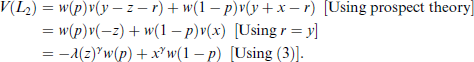
Thus, the indifference in (6) implies that $V (L_{1}) = V (L_{2})$ , or $0 = - λ {(z)}^{γ} w (p) +$ $x^{γ} w (1 - p)$ , so

\begin{matrix} λ = (\frac{w (1 - p)}{w (p)}) {(\frac{x}{z})}^{γ} . \end{matrix}

(7)

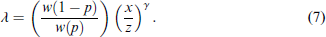
In particular, for the case p = 0.5, that we use in our experimental design, we have $w (1 - p) = w (p) = w (0.5)$ ; hence, from (7) we have that the parameter of loss aversion is

\begin{matrix} λ = {(\frac{x}{z})}^{γ} . \end{matrix}

(8)

We obtain an identical result using linear probability weighting $(w (p) = p)$ .

Remark 1. In our experiments, the elicitation of loss aversion in this section is carried out 'for each individual taxpayer' and separately for each treatment. Hence, (8) written in full notation is $λ_{i j} = {(\frac{x_{i j}}{z})}^{γ_{i j}}$ where $j = L, N$ is an index for the income source, and i is a taxpayer index.

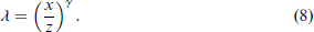
In Equation (8), there are two unknowns on the RHS, x and γ (recall that z was chosen by the experimenter in Equation (6)). We now show how to elicit the preference parameter, γ, of a subject with income y and then we show how to estimate x.

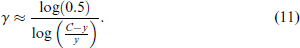
We now describe our theoretical framework for the calculation of γ. We elicit the certainty equivalent value C such that a subject exhibits the following indifference

\begin{matrix} C \sim (y, 0.5; 2 y, 0.5) . \end{matrix}

(9)

The lottery (y,0.5;2y,0.5 offers a 50-50 chance of 'keeping the status-quo income y ' or 'doubling the status-quo income y ' (indeed, such framing, which we use in the experimental instructions, makes the status-quo income salient). The reference income equals the status-quo income y (r = y), so $C \in [y, 2 y]$ . Using r = y, the prospect theory utility function v, defined in (3), and v(0) = 0, the indifference in (9) implies the following prospect theory calculation²⁹

\begin{matrix} v (C - y) = [1 - w (0.5)] v (y - y) + w (0.5) v (2 y - y) . \\ \Rightarrow v (C - y) = w (0.5) v (y) . \end{matrix}

(10)

The two-parameter Prelec probability weighting function $w (p) = e^{- β {(- ln p)}^{α}}$ , where $α, β \geq 0$ , has good empirical support and has axiomatic foundations (Prelec, 1998; al-Nowaihi & Dhami, 2006). Bruhin et al.’s (2010) mixture model estimates of the median values are β = 0.8 and α = 0.45 (this value of α is also consistent with the tax evasion simulations in Dhami & al-Nowaihi, 2007). Evaluated at these parameter values, $w (0.5) = e^{- 0.8 {(- ln 0.5)}^{0.45}} = 0.507$ . Subject-specific estimation of α,β is a very challenging process, so we do not carry out this exercise. Hence, we use the approximation $w (0.5) \approx 0.5$ . In our empirical exercise, we successfully check the robustness of our results to other values of the probability weighting function.

Using Equation (3), and the approximation $w (0.5) \approx 0.5$ , Equation (10) implies ${(C - y)}^{γ} = 0.5 {(y)}^{γ}$ . Solving for γ we get

\begin{matrix} γ \approx \frac{log (0.5)}{log (\frac{C - y}{y})} . \end{matrix}

(11)

Esstimation of x Using the Bisection Procedure

In this section, we outline the subjective estimation of x in Equation (8) following the bisection method. Consider the two lotteries L₁ and L₂ in Equation (6), where y,z, and p are fixed. It is clearer to denote L₂ by L₂(x). Our objective is to find x after offering subjects a series of 6 lottery choices of the following form.

Choice 1: Subjects are given a choice between $L_{1} = (y, 1)$ and $L_{2} (x_{1}) =$ $(y - z, 0.5; y + x_{1}, 0.5)$ , where $x_{1} \in [0, 5 z]$ is determined by equating the expected value of the two lotteries, so $y = 0.5 (y - z) + 0.5 (y + x_{1})$ . Thus, $x_{1} = z$ .

(1.1) If $L_{2} (x_{1})$ is chosen over L₁ we make $L_{2} (x_{1})$ less attractive in the next step by reducing $x_{1} = z$ to $x_{2} = \frac{z}{2}$ , which is the midpoint of $[0, x_{1}]$ (we bisect the interval in each choice, hence, the name 'bisection procedure').

(1.2) If L₁ is chosen over $L_{2} (x_{1})$ , then we make the lottery L₂ more attractive by increasing $x_{1} = z$ to $x_{2} = 3 z$ which is the midpoint of the interval $[x_{1}, 5 z]$ ; the upper limit $5 z$ is picked to be arbitrarily high to accommodate even extreme preferences.

Choice 2: Subjects are given a choice between $L_{1} = (y, 1)$ and $L_{2} (x_{2}) =$ $(y - z, 0.5; y + x_{2}, 0.5)$ , where $x_{2}$ is determined from Choice 1.

(2.1) If $L_{2} (x_{2})$ is chosen over L₁ we make $L_{2} (x_{2})$ less attractive in the next step by reducing $x_{2}$ to $x_{3}$ , which is the midpoint of $[0, x_{2}]$ .

(2.2) If L₁ is chosen over $L_{2} (x_{2})$ , then we make L₂ more attractive by increasing $x_{2}$ to $x_{3}$ which is either the midpoint of the interval $[x_{2}, 5 z]$ (if L₁ was chosen in Choice 1) or $[x_{2}, x_{1}]$ (if $L_{2} (x_{1})$ was chosen in Choice 1).

Choice $k = 3, 4, 5, 6$ : Subjects choose between $L_{1} = (y, 1)$ and $L_{2} (x_{k}) =$ $(y - z, 0.5; y + x_{k}, 0.5)$ , where $x_{k}$ is determined from the previous $k - 1$ choices. Thus, the interval containing x shrinks by either replacing the lower bound or the upper bound of the feasible interval in each iteration based on subjects' choices. The feasible interval in each iteration is contingent on all previous choices.

Estimation of γ Using the Bisection Procedure

In order to estimate λ in Equation (8), we first need to estimate x (which was done above). Then, in order to approximate γ in Equation (11), we elicit the value C such that the indifference in Equation (9) holds. We employ the bisection method with 6 iterations, as in Section III.

Risk Attitudes

The estimation of γ in Section III allows us to elicit data on the subject's risk attitudes as well. The reason is that we have elicited the certainty equivalent C of the lottery $L_{2} = (y, 0.5; 2 y, 0.5)$ , and we know its expected value $E L_{2} =$ 1.5y. Directly comparing C with $E L_{2}$ we can determine if a subject is risk averse $(C < E L_{2})$ or risk loving $(C > E L_{2})$ . Above, we elicited attitudes to risk only in the domain of gains, and not for mixed lotteries that have both gains and losses. Hence, such elicitation of risk attitudes is independent of the parameter of loss aversion.

IV Experimental Design

Our experiments were conducted between March and November 2022 over one-on-one zoom sessions with the experimenter.³⁰ We recruited 525 students from various universities in India. The experiment was programmed in LIONESS, developed by Giamattei et al. (2020).

The payments to the subjects consisted of three components: a show-up fee of Rs. 100 and two incentive-based payments, which were contingent on their choices in the two tasks—the lottery choice task and the tax payment task. On average, subjects took 35 minutes to complete the experiment. The average payment per subject was Rs. 244; thus, the per hour payment, on average, was Rs. 418.³¹ Subjects were assured of strict anonymity of their choices. All subjects were paid in private after the experiment through an automated process which excluded the experimenter, and subjects knew this.

We used a between-subjects design to derive the contrast between our treatments. Subjects are randomly assigned to primed and unprimed groups.³² Subjects in the primed group are asked to read a factually accurate but fairly extreme description of tax evasion in India, with potentially important implications for the provision of critical public services in India.³³ Priming subjects might highlight tax-relevant information and engage descriptive norms of behaviour (e.g. if others evade, I might as well evade) or have an effect on the underlying behavioural parameters. On the other hand, if the information provided in the primed treatment is already readily available to the subjects in the unprimed treatment through their outside-the-lab experiences, then we would expect little effect of priming.

Within the primed and unprimed groups, subjects were randomly allocated to one of the two treatments.³⁴ In treatment T2, subjects could earn 'labour income' by performing a tedious task that required them to count the number of 7s and 9s in different sequences of densely packed numbers in 225 seconds. Based on the number of correct answers, subjects could earn one of the following levels of labour income: 25, 50, 75, 100, 125. To keep the distribution of subjects for each income level comparable in the two treatments, in treatment T1 we randomly allocated subjects to unearned non-labour income levels of 25, 50, 75, 100, 125, using an earlier pilot. This successfully ensured comparable frequencies of subjects for each income level in the two treatments.

Once the income of the subjects was determined (Task 1), they participated in the following two main tasks (Tasks 2 and 3) whose order was randomised. (1) A lottery task that was designed to elicit loss aversion, and (2) a tax payment task in which subjects made a tax evasion decision. We now explain these tasks.

The lottery task

The lottery task was conducted using the income of the subjects from Task 1 (non-labour income in T1 and labour income in T2). The elicitation of the loss aversion parameter, for each subject, is implemented using the process described in Section III.

The tax payment task

Using either their non-labour income (T1) or labour income (T2), we asked subjects to declare their income for tax purposes in response to the following 7 questions. The order of these questions was randomised through a Latin Square Design. For the audit probability function in (1), $p (D) = a - b D$ , $a, b \geq 0$ , we have the following two cases of, respectively, exogenous and endogenous probability of detection. (i) For Q1-Q6, $a > 0, b = 0$ , so $p (D) =$ a. (ii) For Q7, $a > 0, b > 0$ . Note that for most amateur tax evaders, the detection probability ranges between 1% and 5% and the penalty rate θ ranges between 0.5 and 2 (Skinner & Slemrod, 1985). However, in several cases, we explore an even larger range of parameter values in order to achieve a better understanding of the underlying reaction functions of the taxpayers.

Questions Q1-Q3 ask subjects to declare their income for 3 different values of the tax rate (5, 30, and 60%). The audit probability is held fixed at 3% and the fine rate at f = 2, where f = 1 + θ is defined in (2); these are empirically realistic values.

Questions Q4-Q6 ask subjects to declare their income for 3 different values of the fine rate $f = 1 + θ (0, 1$ , and 3). We hold fixed the audit probability at 3% and the tax rate at 30%; these are empirically realistic values. When f = 1, the effective penalty rate is θ = 0 (tax evaders who are caught, pay back just owed taxes), and when f = 3 the effective penalty rate $θ = 2$ . The case $f = 0$ corresponds to $θ = - 1$ , that is, a 100% subsidy to the taxpayer from evasion (if caught, the tax evader pays nothing, not even owed taxes).

Question Q7 asks subject to declare their income under an endogenous detection probability, $p (D) = a - b D, a > 0, b > 0.$ ³⁵ Thus, the probability of audit is decreasing in declared income. The fine rate is held fixed at $f = 2$ and the tax rate at 30%, which are empirically realistic values. We use the parametrisation

\begin{matrix} p (D) = 0.08 - 0.0004 D, \end{matrix}

(12)

so a = 0.08 and b = 0.0004, which satisfies the restrictions in (1). Thus, starting with an exogenous probability of detection of, say, 8%, for every increase in declared income, D, of 25, the probability of detection decreases continuously by 1%. As an example, for someone with an income of 125, who declared their entire income, the detection probability is 3%.

Since the probability of detection is kept fixed for Q1-Q6, the relevant predictions of our model are contained in Proposition 2. Q7 enables us to test the prediction of our more general model (see Proposition 1) based on an audit probability that is decreasing in the amount declared.

Several illustrative examples were given to the subjects to enhance their understanding of the experiments. Subjects also had to answer non-trivial test questions correctly to proceed in the experiment.

V Descriptive Statistics

In this section, we first give general descriptive statistics, followed by our estimates of loss aversion and risk aversion.

Basic Data on Participation and Evasion

Out of 525 people who completed the experiment, 31 people participated twice and we only considered their first attempt. For 3 subjects we have some NAs due to software issues and 14 subjects were not students. Dropping these individuals, we have a sample size of 477.

The number of subjects in each category of income (25, 50,75, 100, 125) for each treatment is shown in Table 1. There is a reasonably similar frequency of subjects in each treatment and the median of income is the same across all 4 treatment arms.

Table 1.

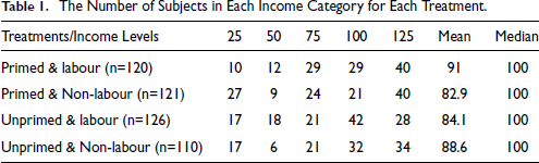
The Number of Subjects in Each Income Category for Each Treatment.

Treatments/Income Levels	25	50	75	100	125	Mean	Median
Primed & labour (n=120)	10	12	29	29	40	91	100
Primed & Non-labour (n=121)	27	9	24	21	40	82.9	100
Unprimed & labour (n=126)	17	18	21	42	28	84.1	100
Unprimed & Non-labour (n=110)	17	6	21	32	34	88.6	100

In Table 2, we report the mean and the medians of the percentage of declared incomes, across all subjects, in all income categories, for each of our 7 questions (see Section IV for a detailed description of the questions). The supplementary section provides details on the corner solutions (D = 0, D = W) and shows that no order effects were found.

Table 2.

Percentage of Declared Income for Each Question.

Treatments		Q1 (t = 5%)	Q2 (t = 30%)	Q3 (t = 60%)	Q4 (f = 0%)	Q5 (f = 1%)	Q6 (f = 3%)	Q7*
Primed & labour	Mean (Median)	81 (100)	67 (72)	53 (50)	36 (18)	51 (50)	80 (100)	75 (80)
Primed & Non-labour	Mean (Median)	78 (100)	64 (68)	50 (40)	32 (0)	48 (48)	75 (96)	74 (93)
Unprimed & labour	Mean (Median)	77 (100)	59 (60)	49 (47)	34 (6)	45 (40)	76 (99)	73 (80)
Unprimed & Non-labour	Mean (Median)	79 (100)	66 (7I)	53 (50)	40 (24)	48 (50)	74 (96)	69 (80)

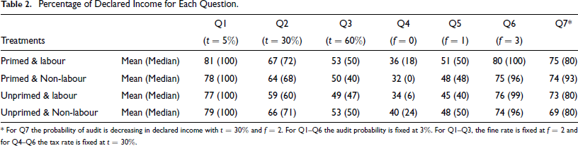
* For Q7 the probability of audit is decreasing in declared income with t = 30% and f = 2. For QI-Q6 the audit probability is fixed at 3%. For QI-Q3, the fine rate is fixed at f = 2 and for Q4-Q6 the tax rate is fixed at t = 30%.

As noted earlier, due to the opposing effects of loss aversion and morality, the overall treatment effects are an empirical question (for an econometric analysis, with controls, see Section VI below). Yet, positive treatment effects (lower evasion for labour income) will indicate to us that loss aversion plays a relatively more important role than moral costs of evasion. In Table 2, there are examples of significant differences in evasion across treatments that should not arise in the absence of source-dependent evasion, or mental accounting. In Q2, and for unprimed subjects, there is a statistically significant difference in declared incomes across the two income sources (3^rd and 4^th rows of column labeled Q2) with p = 0.0396.³⁶ In Q6, and for primed subjects, there is a statistically significant difference in declared incomes across the two income sources (1^st and 2^nd rows of column labelled Q6) with p = 0.0458.

Across all questions, once primed, subjects declare more labour income (58%) as compared to non-labour income (51%). Among the unprimed group, subjects declare more non-labour income as compared to labour income in Q1-Q5.³⁷

In order to compare the differences in declared incomes arising from exogenous and endogenous probabilities of detection (respectively the cases a > 0, b = 0 and a,b > 0), keeping fixed tax rates and penalties at empirically realistic levels (30% tax rate and a fine rate of 3), we compare the results for Q2 and Q7. For the unprimed group, the difference between declared incomes in Q7 and Q2 is greater for labour income as compared to non-labour income (73-59 = 14 in 3^rd row as compared to 69-66 = 3 in 4^th row) suggesting source-dependent tax evasion.

Loss Aversion and Risk Aversion

Our measurement of loss aversion is described in Section III; see Equation (8). Our estimates of mean and median loss aversion are 1.46 and 1.06 respectively.³⁸ This figure is lower than other estimates of loss aversion in the literature that assume a linear utility function. Most estimates of the prospect theory utility function report close to a linear utility function, at least for small stakes (Dhami, 2019, Vol. 1). Under a linear utility function, the mean of loss aversion for our data is 1.83. Chapman et al. (2024) report median values of loss aversion between 1.5 and 2.5 in their survey of the literature. For our data, and employing a non-linear utility function as described above in Section III, the median value of loss aversion is 1.05 for non-labour income (T1) and 1.17 for labour income (T2). The mean value of loss aversion, under a non-linear utility function, in our data, is 1.37 in T1 (non-labour income) and 1.53 in T2 (labour income).³⁹ These figures are consistent with our first conjecture about higher loss aversion for labour income (see (5)).

Chapman et al. (2024) use data for 2000 US respondents on MTurk to measure loss aversion using a new procedure (DOSE). They find a nearly equal split between loss averse (λ > 1) and loss tolerant (λ ≤ 1) individuals. By contrast, a comparison of 8 lab studies shows that loss averse subjects range from 70 to 83% of the total; the rest, 13% to 30%, are loss tolerant.⁴⁰ We find that 52% of our student subjects in T1 and 58% in T2 are loss averse. We follow the Chapman et al. (2024) binary distinction between loss averse ( $λ > 1$ ) and loss tolerant $(λ \leq 1)$ subjects, and use it in our econometric analysis in Section VI. This is likely to mitigate measurement errors, and the effect of extreme strategic responses in the lottery choice task.⁴¹ We also show in the supplementary section that our results are qualitatively similar when we have a continuous measure of loss aversion.

Recall that our risk aversion measure was obtained by using lotteries in the gains domains only so as not to confound its measurement with loss aversion.⁴² We have the following contingency values. Of the loss averse subjects, 193 are risk averse and 69 are risk loving. Of the loss tolerant subjects, 104 are risk averse and 111 are risk loving. The value of Cramér's V (a measure of association between two categorical variables) is 0.2596, indicating low association between risk aversion and loss aversion, allowing for their simultaneous use in the Tobit regressions in Section VI.

Comparative Static Results for t,θ

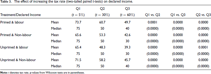
In this section, we analyze the effect on declared income as we vary the tax rate, t, and the penalty rate, θ. The relevant questions are Q1-Q6, with an exogenously fixed probability of detection $(p (D) = a > 0)$ ; the relevant predictions are stated in Proposition 2. An increase in the audit penalty θ is predicted to reduce evasion (Proposition 2b) and an increase in the tax rate t is predicted to increase evasion (Proposition 2c). These results are not new, but they allow us to check that our basic comparative static results are in line with our predictions, and with other findings in the literature.

The Effect of Increasing the Tax Rate

Table 3 shows the average of declared incomes across all treatments for Q1-Q3, with respective tax rates t = 5%,30% and 60%. We keep fixed the penalty rate θ = 1 and the audit probability p = a = 3%, b = 0). We find that the declared income goes down with an increase in the tax rate, which is consistent with our model. Thus, there is no Yitzhaki puzzle under prospect theory (Proposition 2c), in line with the evidence, while there is a predicted Yitzhaki puzzle under expected utility theory and under reasonable attitudes to risk. There is a significant fall in the declared income when the tax rate goes up from 5 to 30%; from 5 to 60%; and from 30 to 60% ( $p <$ 0.000 for all cases). These results are consistent with other empirical results (see the introduction) that report a positive relation between evasion and tax rates.

Table 3.

The effect of increasing the tax rate (two-tailed paired t-tests) on declared income.

		Q1 (t = 5%)	Q2 (t = 30%)	Q3 (t = 60%)	Q1 vs. Q2	Q1 vs. Q3	Q2 vs. Q3
Treatment/Declared Income		73.7	60.7	49.7	0.0001	0.0000	0.0000
Primed & labour	Mean	75	50	40	(0.0000)	(0.0000)	(0.0000)
	Median	65.6	53.3	42.6	0.0000	0.0000	0.0000
Primed & Non-labour	Mean	75	50	30	(0.0000)	(0.0000)	(0.0000)
	Median	65.4	48.3	39.3	0.0000	0.0000	0.0001
Unprimed & labour	Mean	75	50	30	(0.0000)	(0.0000)	(0.0000)
	Median	71.5	58.2	45.7	0.0000	0.0000	0.0000
Unprimed & Non-labour	Mean	75	50	40	(0.0000)	(0.0000)	(0.0000)
	Median	75

Note: t denotes tax rate. p-values from Wilcoxon tests are in parentheses.

Effect of Increasing the Penalty Rate

Table 4 compares declared income across treatments as the fine rate $f = 1 + θ$ is varied from 0,1 to 3 (or, equivalently, as the penalty rate θ is varied from $- 1, 0$ to 2). We keep fixed the tax rate $(t = 30 %)$ and the audit probability ( $p = a = 3 %, b = 0$ ). Even when $θ = - 1$ , that is, there is a 100% subsidy to tax evasion, on average, 35% of the income is declared for tax purposes.⁴³ This is consistent with the presence of moral costs of tax evasion.

Table 4.

The Effect of Increasing the Fine Rate, f (Two-Tailed Paired t-Tests) on Declared Income.

		Q4 (f = 0)	Q5 (f = 1)	Q6 (f = 3)	Q4 vs. Q5	Q4 vs. Q6	Q5 vs. Q6
Treatment/Declared Income		32.5	46.4	73.9	0.0000	0.0000	0.0000
Primed & labour	Mean	10	50	75	(0.0000)	(0.0000)	(0.0000)
	Median	30.1	40.9	63.4	0.0000	0.0000	0.0000
Primed & Non-labour	Mean	1	25	68	(0.0000)	(0.0000)	(0.0000)
	Median	26.6	35.5	65.0	0.0000	0.0000	0.0000
Unprimed & labour	Mean	3.5	25	70	(0.0000)	(0.0000)	(0.0000)
	Median	36.0	42.4	65.4	0.0163	0.0000	0.0000
Unprimed & Non-labour	Mean	20	25	71	(0.00413)	(0.0000)	(0.0000)

Note: f denotes fine rate. p-values from Wilcoxon tests are in parentheses.

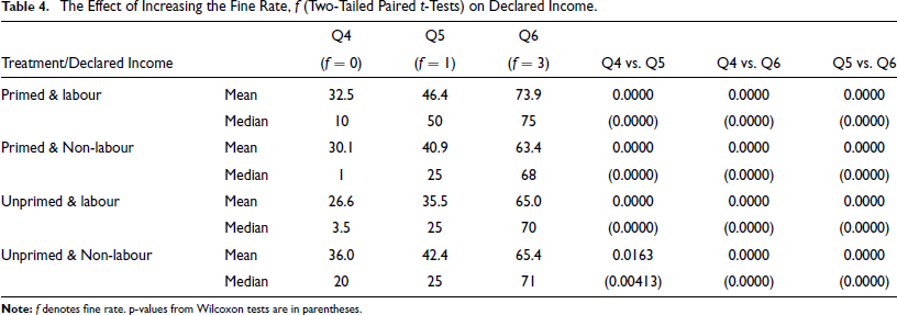
In pairwise comparisons of the declared incomes for Q4, Q5 and Q6, there is a significant increase in the declared incomes when the fine rate increases from 0 to 1, and 3 ( $p < 0.02$ for all pairwise comparisons). The observed positive association between the fine rate and declared income across all treatments is consistent with our theoretical prediction (Proposition 2b).

VI Regression Analysis of the Determinants of Declared Income

Table 6 gives the results of the Tobit regression analysis with robust standard errors for data that is pooled across all questions.⁴⁴ Since we have 5 different levels of incomes, and taxpayers make their declaration decision based on their level of income, we use the proportion of declared income, $Z = D / W$ , as our dependent variable; in this section we shall refer to it as simply 'declared income' instead of the longer 'proportion of declared income'⁴⁵ The relevant predictions are summarised in Proposition 1 and Proposition 2. We run a Tobit regression of the form

\begin{matrix} Z = β X + u, \end{matrix}

(13)

where u is normally distributed with mean zero and variance normalised to unity; X is a vector of explanatory variables and β is a vector of coefficients. The explanatory variables used in (13), with the corresponding names given in Table 6, and the basic data on the individual categories, are as follows.

$d_{λ}$ , or 'Loss aversion': Dummy variable that takes the value 1 if the subject is loss averse $(λ > 1)$ and 0 if the subject is loss tolerant $(λ \leq 1)$ . This classification follows Chapman et al., (2024); see the discussion in Section V. However, we demonstrate the robustness of our results to a continuous measure of loss aversion in the supplementary section.⁴⁶

$d_{R}$ , or 'Risk aversion': Dummy variable that captures attitudes to risk. It takes the value 1 for risk averse individuals and 0 for risk loving individuals.⁴⁷

$d_{T}$ , or 'labour': Treatment dummy that equals 0 for treatment T1 (non-labour income) and 1 for treatment T2 (labour income).

$d_{P}$ , or 'Prime': Treatment dummy that equals 0 for unprimed and 1 for the primed group.

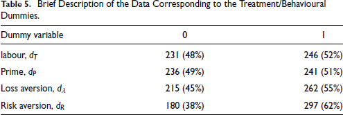
Table 5 gives the data on the different categories of the dummy variables listed above. We have a fairly even distribution across the relevant categories.

Table 5.

Brief Description of the Data Corresponding to the Treatment/Behavioural Dummies.

Dummy variable	0	1
labour, $d_{T}$	231 (48%)	246 (52%)
Prime, $d_{p}$	236 (49%)	241 (51%)
Loss aversion, $d_{λ}$	215 (45%)	262 (55%)
Risk aversion, $d_{R}$	180 (38%)	297 (62%)

Probability of detection: Dummy variable that equals to 1 for endogenous audit probability ( $p = a - b D, a, b > 0$ ); and 0 when there is an exogenous probability of detection ( $p = a; a > 0, b = 0$ ).

Income: Continuous variable corresponding to different level of income received during the experiment.

We also use the interaction terms: $d_{λ} d_{T}, d_{λ} d_{R}, d_{R} d_{T}, d_{λ} d_{R} d_{T}$ . The names of the interaction terms are self explanatory, for example, $d_{λ} d_{T}$ is named Loss aversion:labour and $d_{λ} d_{R}$ is named Loss aversion:Risk aversion.

'Time' indicates the length of time taken for the completion of the experiment.

'Age' gives the self-reported age of subjects. The minimum age is 18, the maximum is 37, mean age is 21.6, median is 20, and the standard deviation is 2.80.

'Gender' is a dummy for gender and takes the value 1 for female and 0 for male; Two hundred forty-five out of four hundred seventy seven subjects (51%) are males and $232 / 477$ subjects (49%) are females (there are $7 / 477$ transgenders/others that are classified as females in the regression).

'Marital' is a dummy for marital status and takes the value 0 for single and 1 otherwise. Since our sample consists of students, most are single 464/477 (97%). Seven subjects are married, 2 subjects are in a domestic relationship and 4 have indicated 'other' for their marital status.

'Religion' is a dummy for religion. It equals 1 for Hindu subjects and 0 otherwise. The majority of our sample is Hindus 335/477 (70%) (Hindus are approximately 80% of the Indian population). Others in the sample subscribe to Islam (4%), Christianity (3%), Jainism (4%), Sikhism ( $0.8 %$ ), Atheism (11%), something else ( $1.8 %$ ) and the rest choose 'I don't want to say it' as their religion (6%).

'Education' is a dummy variable. It equals 1 for Masters/PhD students, and 0 otherwise. 221/477 subjects (46%) are graduate students, and 256/477 subjects (54%) are undergraduates.

In the supplementary section, we successfully demonstrate the robustness of our results to the following extensions. (1) Measurement of the loss aversion parameter on a continuous scale. (2) Different parameters for the probability weighting function used to estimate loss aversion. (3) Using a continuous measure of risk aversion. (4) Using different model specifications.

In Table 6, we describe 3 successively more complex econometric models. In Model 1, we only include the deterrence parameters, loss aversion, risk aversion and the treatment dummies (labour and Prime) as the explanatory variables. None of the treatment dummies are significant at 5%. In Model 2, we add several individual-specific covariates, such as time, age, gender, marital, education and religion. In our most general specification, in Model 3, we also include the interaction terms between various dummy variables (these are $d_{λ} d_{T}, d_{λ} d_{R}, d_{R} d_{T}$ and $d_{λ} d_{R} d_{T}$ ). None of the signs of the regressors changes as we successively include new variables, although their magnitudes and sometimes their significance levels may change. Below, we report on the results from our most complete model, Model 3.⁴⁸

Table 6.

Tobit Regression Results.

	Dependent Variable:
	Proportion of Declared Income
	(I)	(2)	(3)
Tax rate	-1.035***	-1.030***	-1.030***
Tax rate	(0.082)	(0.082)	(0.082)
Fine rate	0.290***	0.290***	0.290***
Fine rate	(0.018)	(0.018)	(0.018)
Probability of detection	0.058**	0.065**	0.066**
Probability of detection	(0.028)	(0.028)	(0.028)
Loss aversion	0.052	0.028	0.181*
Loss aversion	(0.044)	(0.042)	(0.095)
Risk aversion	-0.070	-0.044	-0.018
Risk aversion	(0.046)	(0.044)	(0.089)
labour	0.0003	0.022	0.050
labour	(0.045)	(0.042)	(0.090)
Prime	0.039	0.055	0.053
Prime	(0.045)	(0.044)	(0.043)
Income		-0.0001	-0.0001
Income		(0.001)	(0.001)
Time		-0.005***	-0.005***
Time		(0.002)	(0.002)
Age		0.045***	0.046***
Age		(0.011)	(0.01 I)
Gender		0.208***	0.212***
Gender		(0.044)	(0.044)
Marital		0.201	0.194
Marital		(0.130)	(0.128)
Education		-0.119**	-0.121**
Education		(0.055)	(0.055)
Religion		0.086*	0.096**
Religion		(0.049)	(0.049)
Loss aversion:Risk aversion			-0.192
Loss aversion:Risk aversion			(0.124)
Loss aversion:labour			-0.243*
Loss aversion:labour			(0.135)
Risk aversion:labour			-0.014
Risk aversion:labour			(0.120)
Loss aversion:Risk aversion:labour			0.283
Loss aversion:Risk aversion:labour			(0.172)
logSigma	-0.398***	-0.425***	-0.427***
logSigma	(0.036)	(0.035)	(0.035)
Constant	0.540***	-0.359	-0.410*
Constant	(0.068)	(0.233)	(0.238)
Observations	3339	3339	3339
Log-likelihood	-3094.219	-3016.138	-3009.44
Akaike Inf. Crit.	6206.438	6064.275	6058.88

Notes: *P <.1; **P<.05; ***P<.01. Standard errors are clustered at the individual level (the level of randomisation) and are reported in parentheses.

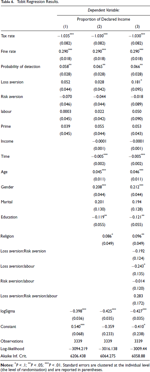
We first verify two effects that we have already demonstrated in Section V above, and are predicted by our model (Proposition 1 and Proposition 2). An increase in the tax rate reduces declared income, which is consistent with prospect theory, but not with expected utility theory (Yitzhaki puzzle). An increase in the fine rate increases declare income. Both are statistically significant at 1%.

Recall our discussion about ambiguous treatment effects predicted by economic theory, hence, the treatment effect is an empirical question. We find that taxpayers declare 5% more labour income relative to non-labour income. Thus, overall and in terms of the direct effect, loss aversion dominates morality costs in inducing greater declaration of labour income. Taxpayers declare, on average, $6.7 %$ more of their income when there is an endogenous probability of detection (that depends on the amount declared) relative to an exogenous probability of detection. Several control variables such as time, age, gender, religion and education are significant. Those who spend more time deliberating on the declaration decision, declare lower income, but the effect is small. Those who are older declare more; a unit increase in age (measured in years) increases declared income by 4.6%. Females declare 21.2% more income relative to males. This ties in with the literature on gender differences in economic decisions including the greater tendency of males to be more overconfident and take more risks (Dhami, 2016); we extend these results to illegal activity.

The more educated students declare less income; Masters/PhD students reduce declared income by $12.1 %$ , relative to others with lower educational qualifications. This is an interesting result and deserving of greater exploration in future research. Primed subjects declare $5.3 %$ more income relative to unprimed subjects.⁴⁹ Those who give their religion as 'Hindu' declare 9.6% more income relative to those who do not.⁵⁰

Loss aversion, on its own, is significant and increases declared incomes. In terms of the direct effect, those who are loss averse declare $18.1 %$ more of their income, relative to those who are loss seeking. This finding is consistent with our theory and our proposed transmission mechanism behind mental accounting, based on loss aversion. We provide the first direct empirical evidence, using subject-specific, directly measured, loss aversion, for the underlying transmission channel in most 'prospect theory based' explanations of tax evasion (Bernasconi, 1998; Yaniv, 1999; Bernasconi & Zanardi, 2004; Dhami & al-Nowaihi, 2007, 2010; Eide et al., 2011; Alm & Torgler, 2012; Engström et al., 2015; Rees-Jones, 2018). Risk aversion by itself, is not significant and the magnitude of the effect on declared incomes is small at $1.8 %$ . But it has an important role to play through its interaction effects with other variables, as we show below. The interaction between loss aversion and the treatment dummy $(d_{λ} d_{T})$ is significant. If the taxpayer treated both sources of income in an identical manner, which would be the case if mental accounting were absent, then we should not have obtained statistical significance for this variable. Since the determinants of tax evasion are dependent on the source of income, this supports a mental accounting-based explanation of tax evasion that we are interested in. However, our analysis of mental accounting goes beyond just identifying source-dependent evasion. We highlight the main channels, loss aversion and risk aversion, through which mental accounting works, and empirically verify it.

We now use Table 6 to identify several effects arising from the interaction of the dummy variables in our model. We use the notation $E (Z ∣ d_{T}, d_{λ}, d_{R})$ to denote the average declared income, conditional on different values of the three conditioning dummy variables, $d_{T}, d_{λ}, d_{R} .$ ⁵¹

The main result of interest, from a treatment effect point of view, is the average differences in the declared amounts of loss averse subjects $(d_{λ} = 1)$ as we vary the two sources of incomes, labour income $(d_{T} = 1)$ and non-labour income $(d_{T} = 0)$ . However, we also condition on risk attitudes: risk averse $(d_{R} = 1)$ and risk loving $(d_{R} = 0)$ .

Loss averse taxpayers, $d_{λ} = 1$ , who are risk averse, $d_{R} = 1$ .

E (Z | d_{T} = 1, d_{λ} = 1, d_{R} = 1) - E (Z | d_{T} = 0, d_{λ} = 1, d_{R} = 1) = 0.076.

(14)

From (14), restricting attention to loss averse $(d_{λ} = 1)$ and risk averse $(d_{R} = 1)$ taxpayers, subjects declare $7.6 %$ more income when they earn labour income $(d_{T} = 1)$ relative to non-labour income $(d_{T} = 0)$ . This effect, in conjunction with our earlier finding in Section V on higher average loss aversion for labour income, is consistent with our main assumption on the transmission channel based on loss aversion.

Loss averse taxpayers, $d_{λ} = 1$ , who are risk loving, $d_{R} = 0$ .

\begin{matrix} E (Z | d_{T} = 1, d_{λ} = 1, d_{R} = 0) - E (Z | d_{T} = 0, d_{λ} = 1, d_{R} = 0) = - 0.193. \end{matrix}

(15)

From (15), loss averse subjects, who are also risk loving, declare 19.3% less of their labour incomes as compared to their non-labour incomes. Comparing (14) and (15), risk aversion strengthens the cautionary effect of loss aversion, while risk loving behaviour attenuates, and even reverses the effect of loss aversion. As far as we are aware, this is the first demonstration of such a result in the literature on decision making under risk and uncertainty, based on directly measured subject-specific loss aversion and risk aversion.

The results in (14) and (15), since they directly reveal evasion differences for two different sources of income, that are identical in all other respects, support our claims on source-dependent mental accounting in this study. A similar comment applies to the results below.

Loss seeking taxpayers, $d_{λ} = 0$ , who are risk averse $d_{R} = 1$ .

E (Z | d_{T} = 1, d_{λ} = 0, d_{R} = 1) - E (Z | d_{T} = 0, d_{λ} = 0, d_{R} = 1) = 0.036.

(16)

From (16), restricting attention to loss seeking $(d_{λ} = 0)$ and risk averse $(d_{R} = 1)$ taxpayers, subjects declare $3.6 %$ more income when they earn labour income $(d_{T} = 1)$ relative to non-labour income $(d_{T} = 0)$ . Comparing with the case of loss averse subjects in (14), loss seeking subjects declare lower incomes. This is consistent with our predictions. In this case, the cautionary effects of risk aversion counter the opposing effect of loss seeking behaviour.

Loss seeking taxpayers, $d_{λ} = 0$ , who are risk loving, $d_{R} = 0$ .

E (Z | d_{T} = 1, d_{λ} = 0, d_{R} = 0) - E (Z | d_{T} = 0, d_{λ} = 0, d_{R} = 0) = 0.050.

(17)

From (17), restricting attention to loss seeking $(d_{λ} = 0)$ and risk loving $(d_{R} = 0)$ taxpayers, subjects declare $5.0 %$ more income when they earn labour income $(d_{T} = 1)$ relative to non-labour income $(d_{T} = 0)$ . The comparison between (15) and (17) is interesting and difficult to reconcile with known theory. Loss aversion interacts with risk loving behaviour to produce lower declared labour incomes relative to non-labour incomes in (15); we have conjectured the reasons, above. However, loss seeking interacts with risk seeking to produce relatively higher declared labour incomes in (17). It would appear that the interaction between loss aversion, risk aversion and mental accounting of incomes is complex and requires new further developments.

VII Conclusions

Our main contribution is to provide the first rigorous demonstration of a link between subject specific loss aversion and tax evasion, which lies at the heart of many modern theories of tax evasion.

There are several novel features of our analysis. First, we derive theoretical predictions for tax evasion by exploiting the link between loss aversion, risk aversion, mental accounting and moral costs in a prospect theory framework. Second, we propose a theoretical framework for measuring subject-specific loss aversion; and empirically determine a strategy to measure it that is independent of risk aversion. Third, a combination of loss aversion, moral costs and risk aversion is essential for an understanding of tax evasion that depends on the source of income. For instance, it appears that risk aversion strengthens the cautionary effect of loss aversion, while risk loving behaviour attenuates the effect of loss aversion. However, a third dimension, the source of income, makes it difficult to present truly generalised findings. Fourth, our empirical results show that entitlements to income influence the degree of evasion (source-dependent evasion). Fifth, we show that the effectiveness of loss aversion in reducing evasion is income-source specific. The interactions of the treatment effect with loss/risk attitudes are significant. These findings suggest the importance of mental accounting. Sixth, we confirm the predicted comparative static effects of the probability of detection, the penalty rate and the tax rate on tax evasion for the same set of subjects, for two different sources of income.

While we are able to explain most of our results, our model is unable to provide explanations of some of the results. This is the case with our finding of new and unknown interaction effects of risk aversion with loss aversion that are income source dependent. This requires further developments in the relevant theory.

Footnotes

Acknowledgement

We are extremely grateful to James Alm, Junaid Arshad, Michele Bernasconi, and Alex ReesJones for their comments and suggestions on earlier versions of the paper. We are grateful to the Centre for Social and Behaviour Change (CSBC), Ashoka University for their facilities. The experiments were run and funded by the CSBC Lab at Ashoka and we thank Bijoyetri Samaddar and Aayush Agarwal for their superb assistance in designing and in the running of experiments.

Declaration of Conflicting Interests

The authors declared no potential conflicts of interest with respect to the research, authorship and/or publication of this article.

Funding

The authors received no financial support for the research, authorship and/or publication of this article.

Supplementary Materials

Notes

References

Abdellaoui

(2000). Parameter-free elicitation of utility and probability weighting function. Management Science , 46(11): 1497–1512.

al-Nowaihi

, Bradley

, & Dhami

(2008). A note on the utility function under prospect theory. Economics Letters , 99(2): 337–339.

al-Nowaihi

, & Dhami

(2006). A simple derivation of Prelec's probability weighting function. Journal of Mathematical Psychology , 50(6): 521–524.

Allingham

M. G.

, & Sandmo

(1972). Income tax evasion: A theoretical analysis. Journal of Public Economics , 1(3-4): 323–238.

Alm

(2019). What motivates tax compliance. Journal of Economic Surveys , 33(2): 353–388.

Alm

, & Torgler

(2012). Do ethics matter? Tax compliance and morality. Journal of Business Ethics , 101(4): 635–651.

Alm

, & Malézieux

(2021). 40 years of tax evasion games: A meta-analysis. Experimental Economics , 24: 699–750.

Andreoni

, Erard

, & Feinstein

(1998). Tax compliance. Journal of Economic Literature , 36(2): 818–860.

Bernasconi

(1998). Tax evasion and orders of risk aversion. Journal of Public Economics , 67(1): 123–134.

10.

Bernasconi

, & Zanardi

(2004). Tax evasion, tax rates and reference dependence. Finanz Archiv , 60(3): 422–445.

11.

Blake

, Cannon

, & Wright

(2021). Quantifying loss aversion: Evidence from a UK population survey. Journal of Risk and Uncertainty , 63: 27–57.

12.

Brown

A. L.

, Imai

, Vieider

, & Camerer

C. F.

(2023). Meta-Analysis of Empirical Estimates of Loss-Aversion. Forthcoming in Journal of Economic Literature .

13.

Bruhin

, Fehr-Duda

, & Epper

(2010). Risk and rationality: Uncovering heterogeneity in probability distortion. Econometrica , 78(4): 1375–412.

14.

Cappelen

A. W.

, Hole

A. D.

, Sørensen

E. Ø.

, & Tungodden

(2007). The pluralism of fairness ideals: An experimental approach. American Economic Review , 97(3): 818–827.

15.

Chapman

, Snowberg

, Wang

, & Camerer

(2024). Looming Large or Seeming Small? Attitudes Towards Losses in a Representative Sample . Mimeo Bologna University.

16.

Cherry

T. L.

, Frykblom

, & Shogren

J. F.

(2002). Hardnose the dictator. American Economic Review , 92(4): 1218–1221.

17.

Clotfelter

C. T.

(1983). Tax evasion and tax rates: An analysis of individual returns. Review of Economics and Statistics , 65(3): 363–373.

18.

Dhami

(2019). Foundations of behavioral economic analysis: Volume I: Behavioral Decision Theory . Oxford University Press: Oxford.

19.

Dhami

(2019). Foundations of behavioral economic analysis: Volume II: Other-Regarding preferences . Oxford University Press: Oxford.

20.

Dhami

(2020). Foundations of behavioral economic analysis: Volume V: Bounded Rationality . Oxford University Press: Oxford.

21.

Dhami

, & al-Nowaihi

(2007). Why do people pay taxes: Expected utility versus prospect theory. Journal of Economic Behaviour and Organization , 64(1): 171–192.

22.

Dhami

, & al-Nowaihi

(2010). Optimal income taxation in the presence of tax evasion: Expected utility versus prospect theory, with Ali al-Nowaihi. Journal of Economic Behavior and Organization , 75(2): 313–337.

23.

Dhami

, Manifold

, & al-Nowaihi

(2020). Identity and redistribution: Theory and evidence. Economica , 88(350): 499–531.

24.

Dhami

, & Sunstein

C. R.

(2022). Bounded rationality: Heuristics, judgment, and public policy . MIT Press: Massachussetts.

25.

Dhami

, Wei

, & Mamidi

(2022). Religious Identity, Trust, Reciprocity, and Prosociality: Theory and Evidence. CESifo Working Paper No. 10147.

26.

Eide

, von Simson

, & Strom

(2011). Rank-dependent utility, tax evasion, and labor supply. FinanzArchiv , 67(3): 261–281.

27.

Engström

, Nordblom

, Ohlsson

, & Persson

(2015). Tax compliance and loss aversion. American Economic Journal: Economic Policy , 7(4): 132–164.

28.

Commission

European

(2019). Estimating International Tax Evasion by Individuals. Working Paper No 76-2019.

29.

Feinstein

J. S.

(1991). An econometric analysis of income tax evasion and its detection. RAND Journal of Economics , 22, 14–35.

30.

Friedland

, Maital

, & Rutenberg

(1978). A simulation study of income tax evasion. Journal of Public Economics , 10(1), 107–116.

31.

Giamattei

, Yahosseini

K. S.

, Gächter

, & Molleman

(2020). LIONESS Lab: A free web-based platform for conducting interactive experiments online. Journal of the Economic Science Association , 6: 95–111.

32.

Hoffman

, & Spitzer

M. L.

(1982). The Coase theorem: Some experimental tests. Journal of Law and Economics , 25(1): 73–98.

33.

Kahneman

, & Tversky

A. (Eds.)

. (2000). Choices, values and frames . Cambridge: Cambridge University Press.

34.

Kahneman

, & Tversky

(1979). Prospect theory: An analysis of decision under risk. Econometrica , 47(2): 263–291.

35.

Lee

, & Shahriar

(2017). Fairness, one's source of income, and others' decisions: An ultimatum game experiment. Managerial and Decision Economics , 38(3): 423–431.

36.

List

J. A.

, & Cherry

T. L.

(2000). Learning to accept in ultimatum games: Evidence from an experimental design that generates low offers. Experimental Economics , 3(1): 11–29.

37.

Novemsky

, & Kahneman

(2005). The boundaries of loss aversion. Journal of Marketing Research , 42(2): 119–28.

38.

Oxoby

, & Spraggon

(2008). Mine and yours: Property rights in dictator games. Journal of Economic Behavior and Organization , 65(3-4): 703–713.

39.

Prelec

(1998). The probability weighting function. Econometrica , 66(3): 497–528.

40.

Rees-Jones

(2018). Quantifying loss-averse tax manipulation. The Review of Economic Studies , 85(2):1251–1278.

41.

Skinner

, & Slemrod

(1985). An economic perspective on tax evasion. National Tax Journal , 38, 345–353.

42.

Slemrod

, & Yitzhaki

(2002). Tax avoidance, evasion and administration. In: Auerbach

A. J.

, & Feldstein

(Eds.). Handbook of Public Economics , Vol. 3. Amsterdam: Elsevier Science, chapter 22, 1423–1470.

43.

Thaler

R. H.

(1999). Mental accounting matters. Journal of Behavioral Decision Making , 12(3): 183–206.

44.

Tversky

, & Kahneman

(1992). Advances in prospect theory: Cumulative representation of uncertainty. Journal of Risk and Uncertainty , 5(4): 297–323.

45.

Wakker

P. P.

(2010). Prospect theory: For risk and ambiguity . Cambridge University Press: Cambridge.

46.

Yaniv

(1999). Tax compliance and advance tax payments: A prospect theory analysis. National Tax Journal , 52(4): 753–764.

47.

Yitzhaki

(1974). A note on income tax evasion: A theoretical analysis. Journal of Public Economics , 3(2): 201–202.

48.

Yoder

K. J.

, & Decety

(2018). The neuroscience of morality and social decision-making. Psychology, Crime and Law , 24(3): 279–295.

Supplementary Material

Please find the following supplemental material available below.

For Open Access articles published under a Creative Commons License, all supplemental material carries the same license as the article it is associated with.

For non-Open Access articles published, all supplemental material carries a non-exclusive license, and permission requests for re-use of supplemental material or any part of supplemental material shall be sent directly to the copyright owner as specified in the copyright notice associated with the article.

0.00 MB

0.34 MB

Loss Aversion and Tax Evasion: Theory and Evidence

Abstract

Keywords

I Introduction

Loss Aversion and Tax Evasion

Source-Dependent Evasion

Loss Aversion and Risk Aversion

Theoretical Model

Experiments and Findings

Schematic Outline of Paper

II The Model

Theoretical Framework for Estimating Loss Aversion

Esstimation of x Using the Bisection Procedure

Estimation of γ Using the Bisection Procedure

Risk Attitudes

Basic Data on Participation and Evasion

Table 1.

The Number of Subjects in Each Income Category for Each Treatment.

Percentage of Declared Income for Each Question.

Loss Aversion and Risk Aversion

Comparative Static Results for t,θ

The Effect of Increasing the Tax Rate

The effect of increasing the tax rate (two-tailed paired t-tests) on declared income.

Effect of Increasing the Penalty Rate

The Effect of Increasing the Fine Rate, f (Two-Tailed Paired t-Tests) on Declared Income.

Brief Description of the Data Corresponding to the Treatment/Behavioural Dummies.

Tobit Regression Results.

Footnotes

Acknowledgement

Declaration of Conflicting Interests

Funding

Supplementary Materials

Notes

References

Supplementary Material