
Abstract
The focus of this article is on the ‘educational attainment’ of social groups in India, defined as the proportion of 21–29-year-olds in the different social groups that are graduates. Within this context, the article makes three contributions. The first is in terms of decomposition methodology: It shows how decomposition analysis can be used to breakdown graduate educational attainment (GEA) by population subgroups and region to offer insight into the policy levers available for improving the GEA of certain groups. The second is to a methodology for computing probabilities (termed ‘recycled predictions’) for isolating the group-specific probabilities of GEA which can be totally attributed to group identity. The third is to use these probabilities to break down the differences in proportions between social classes into a ‘social group effect’ and an ‘endowments effect’. The data for this article is from India’s Periodic Labour Force Survey for the period 2017–2018.
Introduction
It is fairly well-recognized that the educational achievements of young people in India vary according to the social group to which they belong, whether these achievements are measured by the proportion of (a) 21–29-year-olds that are graduates, (b) 15–24-year-olds that are enrolled in educational institutions or (c) young persons that are not in employment, education or training (NEET). This matters because education is an important input to personal development, and inclusive growth [sabka saath, sabka vikas] requires that no group should be systemically left behind in acquiring education. A recent report (Angad, 2023) about how the lives of previously illiterate women in Dhumka district in Jharkhand (India) were transformed by helping them acquire skills of literacy and numeracy illustrates the power of education even at a very basic level.
The history of educational achievement largely being the prerogative of upper-caste Indians is a long one. Surveying the importance of caste in the Indian economy, Munshi (2019) argues that in terms of schooling, caste affects school enrolment, attendance and attainment. In terms of enrolment, Borooah and Iyer (2005), using the Indian Human Development Survey data, showed that the effect of religion (Hindu or Muslim) or caste (Scheduled or non-Scheduled) on school enrolment depended very much on the non-group circumstances of children: Under good conditions (say, when parents were educated), the community effect was small; however, under worse circumstances, it could be large. In terms of attainment, Borooah (2012) examined the role of religion and caste in explaining the gap in education among children aged 8–11 in India and concluded that children from the Muslim, Dalit and Adivasi groups were disadvantaged in respect of the three basic competencies of reading, writing and arithmetic, relative to Brahmin children.
A related issue in educational attainment is the effect of ‘negative stereotypes’: Individuals belonging to groups that are expected to do badly (the negative stereotype associated with low castes), do, in fact, perform worse than those belonging to groups that are not negatively stereotyped (upper castes). Hoff and Pandey (2006) showed in an experiment that when caste identity was concealed, lower- and upper-caste children performed equally well on a test, but when the castes of the children were made public, the performance of lower-caste children deteriorated markedly.
Many of the religion- and caste-based inequalities that one observes in schooling in India continue at college and university levels. Even though students from the lower castes, such as the Other Backward Classes (OBC), Scheduled Castes (SC) and Scheduled Tribes (ST), are offered admission to public educational institutions on preferential terms, there is limited access to higher education for Muslims and the lower castes (Borooah, 2017).
This is reflected in the fact that data from the Periodic Labour Force Survey (PLFS), 2017–18 (hereafter, PLFS-2017/18; Ministry of Statistics and Programme Implementation, 2019) shows that, on all the above measures, Muslims fared the worst among India’s social groups with Hindus from the ‘forward castes’ (FC) doing the best (Jaffrelot & Kalaiyarasan, 2019). The proportion of persons who were 21–29 years of age, hereafter referred to as ‘young adults’ and abbreviated to YA who were graduates, was only 14% for Muslims, rising to 18% for the SCs, rising further to 25% for Hindu OBCs and reaching a peak of 37% for Hindu FC. In terms of enrolment, only 39% of Muslim youths (i.e., 15–24 years of age) were currently enrolled in educational institutions compared to 44% of the SCs, 51% of Hindu OBCs and 59% of Hindu FC. At the other end of the educational spectrum, Muslims had the highest percentage of youths who were NEET (31%), followed by 26% for the SCs and 23% and 17% for Hindu OBCs and Hindu FC, respectively.
Against this background of inter-caste and inter-religion inequalities in educational attainment, the purpose of this article is to go behind these figures and attempt to understand why these differences in educational achievement between social groups in India occur. First, there is the question of ‘demand’. Is it the case that certain groups, more than others, see the value of education and are attracted to it? On this issue, people make calculations about the value of education in terms of their personal and social development.
Second, there is the issue of ‘resources’, whether household resources are adequate to enable their young persons to pursue higher education. It may be that spending the necessary years at college to obtain a degree is beyond the household resources of some people. The question is whether households are capable of investing in higher education by foregoing current income and households in different groups arrive at different answers.
The third issue is one of ‘infrastructure’. Regional accessibility can lead to a wide range of direct and indirect costs and can limit participation (Cullinan & Flannery, 2021). If members of certain groups are fortunate/unfortunate enough to be disproportionately located in areas in which the general level of education is high/low then that fact will aid/hinder participation. This article quantifies the effects of location in two ways: (a) a person’s residence in a rural or urban area and (b) the person’s residence in a region of India. With respect to regional location, the 21 major Indian states were aggregated into the following areas: The North (Uttarakhand, Himachal Pradesh, Punjab, Haryana and Jammu and Kashmir), the Central (Rajasthan, Uttar Pradesh, Bihar, Jharkhand, Chhattisgarh and Madhya Pradesh), the East (Assam, West Bengal and Odisha), the West (Maharashtra and Gujarat) and the South (Andhra Pradesh, Telangana, Karnataka, Kerala and Tamil Nadu). Analysis of these three factors—demand, resources and location—collectively in influencing decisions to enter and to remain in higher education may be abbreviated as the DRL model (of higher education participation).
As noted above, there are several measures of educational underachievement, for example, in terms of enrolment in educational institutions or being outside the world of NEET. Given the constraints of journal space in terms of setting out the details of the analysis, the focus of this article is to use the DRL model, in conjunction with data from the PLFS-2017/18, to analyse the proportion YA in India, in different social groups, that are graduates. 1 This proportion is, hereafter, referred to as graduate educational attainment (GEA), and this article seeks to understand why levels of GEA in India differ between youths from different social groups. 2
Within this context, the article makes three contributions. The first contribution is in terms of decomposition methodology. In the third section, the article shows how decomposition analysis can be used to breakdown GEA by population subgroups and region to offer insight on the policy levers available for improving the GEA of certain groups. It constructs an analytic model of decomposition which shows how GEA could depend both on group membership and on non-group related factors.
The second contribution is using a methodology for computing probabilities (termed ‘recycled predictions’) for isolating the group specific probabilities of GEA which can be entirely ascribed to group identity. From this, one obtains the average probability of GEA for five social groups, defined below, such that these probabilities could be regarded as being entirely dependent on group preferences for graduate education.
The third contribution is to compare the ‘computed’ probabilities, based on the method of recycled predictions, for each social group of GEA with the ‘observed’ proportion of graduates from that group. This then allows for a breakdown of the differences in proportions between social classes into a ‘social group effect’ and a ‘endowments effect’. This is consistent with the methodology of Oaxaca (1973), Blinder (1973) and Oaxaca and Ransome (1994) in attributing a gender and an attributes effect to the observed difference in wages between men and women.
Papers which offer a quantitative analysis of social phenomenon often emphasize parsimony and, in so doing, risk missing qualitative features which cannot be easily quantified. This article is no exception. There is often tension between a broad brush picture which omits details and a detailed picture which fails to convey an overall view.
The analysis of GEA by the different social groups in this article is driven by three factors—demand, resources and location—and while this is parsimonious explanation arguably captures the essence of the phenomenon, it misses several relevant factors which may be specific to households. For example, the specification does not include the highest education of a household member which might be an incentive or disincentive for the households’ YA to study further. 3 Again, the analysis does not consider whether female YA are married and constrained by home duties. Neglect of these factors is not to say they are not important, rather that data that can be incorporated in the analysis is often not available in a specific data set or that additional factors that might influence the outcome do not systematically vary by social group.
Data
The data for this article is from the PLFS-2017/18, described in Ministry of Statistics and Programme Implementation (2019). Between July 2017 and June 2018, 102,113 households (56,108 in rural areas and 46,005 in urban areas) were surveyed by the PLFS-2017/18 and this encompassed 433,339 persons (246,809 in rural areas and 186,530 in urban areas). 4 The highlights of the PLFS-2017/18 are set out in detail in Ministry of Statistics and Programme Implementation (2019).
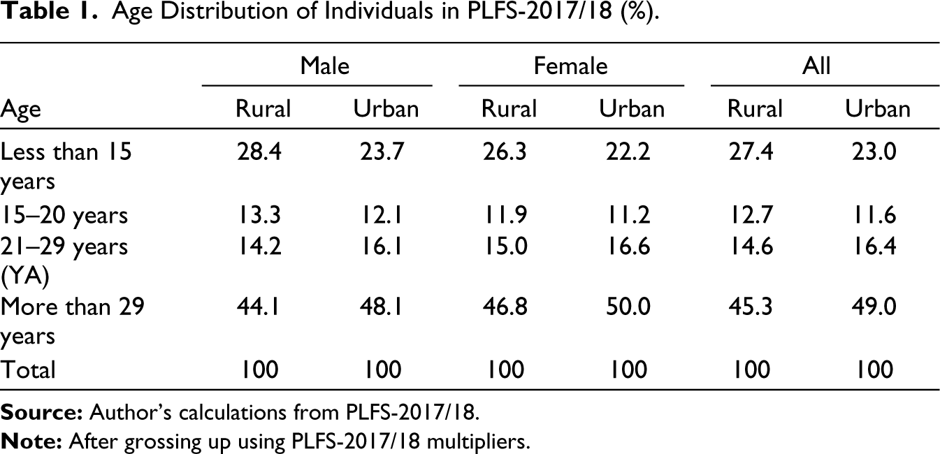
This study focuses on the GEA of those between 21 and 29 years of age. These persons, collectively described as ‘young adults’ (hereafter, YA), comprised 14.2% and 15.0% of rural men and women, respectively, and 16.1% and 16.6% of urban men and women, respectively. Over both genders, YA comprised 14.6% and 16.4% of rural and urban persons, respectively. 5 After grossing up the sample figures by the multiplier weights provided in PLFS-2017/18, Table 1 shows the age distribution of individuals in PLFS-2017/18.
Age Distribution of Individuals in PLFS-2017/18 (%).
The YA were then grouped as ST, SC, Hindu OBC (OBC), Muslims and FC. 6 These groups comprised 9.5% (ST), 19.9% (SC), 36% (OBC), 12.5% (Muslim) and 22.1% (FC) of the sample of YA. It is plausible to assume that infrastructure for higher education in India might be poorer in the rural, than in the urban, sector and, in this regard, YA in the five social groups were unequally located between the two sectors: 40.9% of YA Muslims and 46% of YA from the FC lived in urban areas compared to 12.2% of YA that were ST and 24.8% that were SC.
Educational Attainment by Subgroup
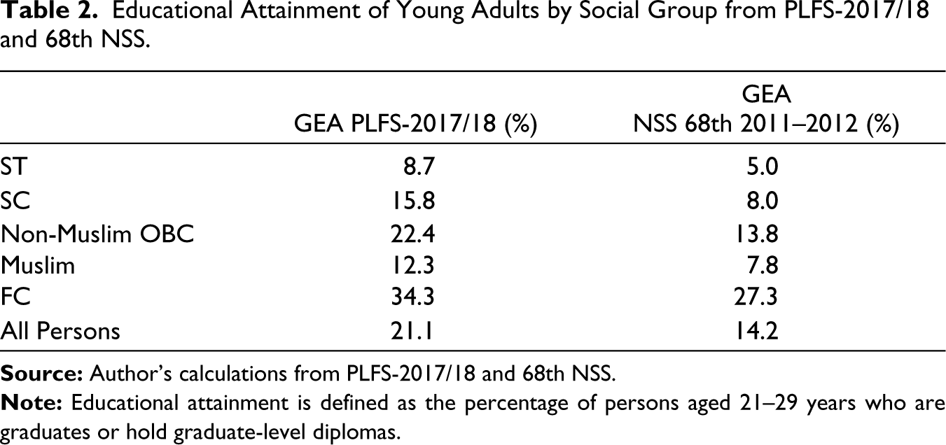
Table 2 shows the GEA of social groups from PLFS-2017/18 and compares it with the groups’ GEA from the 68th Round of the National Sample Survey 2010–2011 (hereafter, 68th NSS). The first point of interest is that there were substantial increases in the GEA of all the social groups: from 5% to 8.7% for the ST; from 8% to 15.8% for the SC; from 13.8% to 22.4% for the OBC; from 7.8% to 12.3% for Muslims; and from 27.3% to 34.3% for the FC. Consequently, the overall GEA in India rose from 14.2% in 2011–2012 to 21.4% in 2017–2018. Notwithstanding these improvements, the ST, SC and Muslims had the lowest levels of GEA in both periods which were substantially lower than that of the FC. 7
Educational Attainment of Young Adults by Social Group from PLFS-2017/18 and 68th NSS.
The hypothesis of this article is that, in respect of GEA, the four non-FC groups—ST, SC, OBC and Muslims—had two disadvantages vis-à-vis the FC: (a) They may have been less enthusiastic about graduate education than their FC counterparts and (b) they may have had less access to graduate education. The enthusiasm displayed by the various social groups for degree level education is termed in this article as their ‘graduate propensity’ (GP). The relative lack of ‘access’ of persons from the non-FC groups to graduate education is hypothesized to stem from two characteristics: (a) a disproportionate presence of non-FC persons in low-income households and (b) a disproportionate presence of non-FC persons in states which had a low EA.
Mean Monthly Consumption Expenditure of YA by Social Group
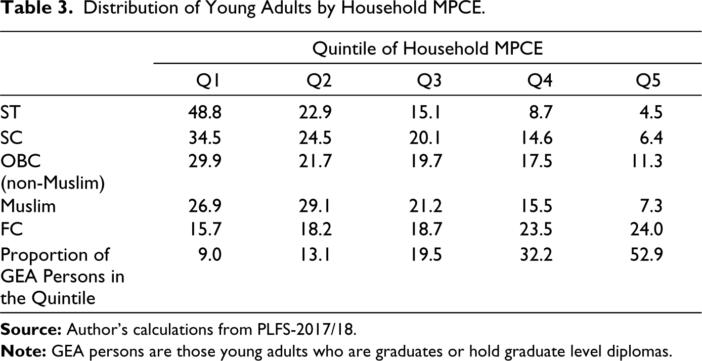
The YA were allotted to one of five quintiles of monthly per capita consumption expenditure (MPCE) depending upon their households’ MPCE. These quintiles were Q1 (lowest) to Q5 (highest), and Table 3 shows the unequal distribution between the MPCE quintiles of persons belonging to the different groups: 24% of YA from the FC were in the highest quintile of household MPCE (with another 23.5% in the next highest quintile); by contrast, only 4.5% of YA from the ST, and 6.4% of YA from the SC, 11.3% of YA from the OBC, and 7.3% of YA Muslims were in the highest quintile of household MPCE. Table 3 also shows the economic rewards associated with being a graduate: Only 9% of YA in Q1 of MPCE and 52.9% YA in Q5 of MPCE were graduates.
Distribution of Young Adults by Household MPCE.
Geographical Dispersion of GEA
The analysis in this sub-section on data considerations was restricted to YA living in India’s 21 major states: Andhra Pradesh, Assam, Bihar, Chhattisgarh, Haryana, Himachal Pradesh, Gujarat, Jammu and Kashmir, Jharkhand, Karnataka, Kerala, Madhya Pradesh, Maharashtra, Odisha, Punjab, Rajasthan, Tamil Nadu, Telangana, Uttar Pradesh, Uttaranchal and West Bengal. 8 Collectively, these states accounted for 96.5% of the sample size.
In terms of geographical dispersion, Table 4 shows that coinciding with the fact that some of the states with the lowest GEA were Assam (11.4% were graduates), Bihar (12.3%), and West Bengal (12.8%). Assam and West Bengal were the states in India with the highest concentration of Muslims: 26% and 27% of the (grossed up) sample in Assam and Bengal were Muslim, and Bihar had a high concentration (52%) of YA from the OBC. Other states with a low GEA were Jharkhand (13.6%), Odisha (12.2%), Chhattisgarh (11.2%) and Madhya Pradesh (16.7%). All four states had a high concentration of YA from the ST in their (grossed up) samples: 29.7% in Jharkhand, 23.1% in Odisha, 31.2% in Chhattisgarh and 21.9% in Madhya Pradesh. Thus, again, it is not unreasonable to suppose that part of the reason for the low GEA in certain states the disproportionate presence of low GEA groups in their populations.
GEA of Young Adults (YA) by State and Region.
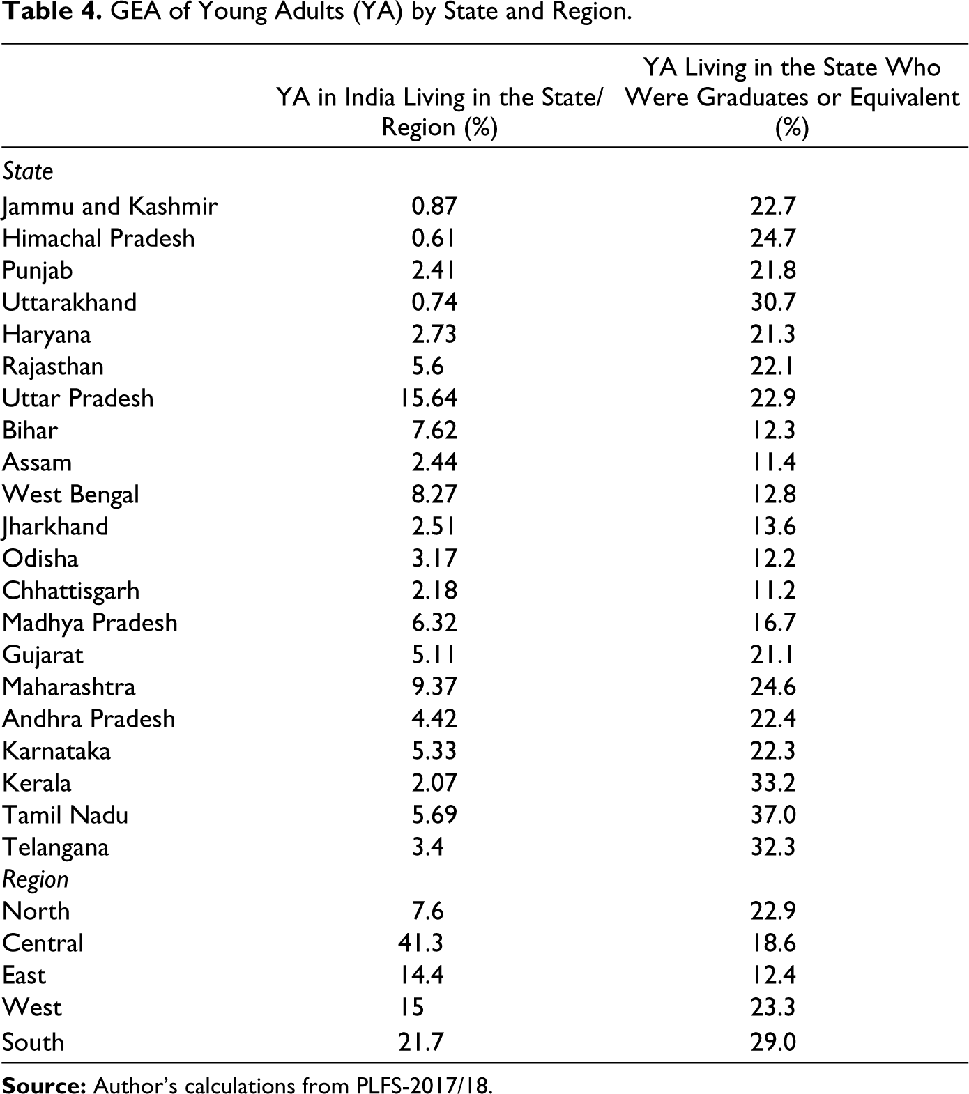
The 21 major states were aggregated, for purposes of the econometric analysis reported in the next section, into five broad regions: North (Jammu and Kashmir, Uttarakhand, Himachal Pradesh, Punjab and Haryana), Central (Rajasthan, Uttar Pradesh, Bihar, Jharkhand, Chhattisgarh and Madhya Pradesh), East (Assam, West Bengal, Odisha), West (Gujarat and Maharashtra) and South (Andhra Pradesh, Telangana, Karnataka, Kerala and Tamil Nadu). Table 4 shows that the South, with 21.7% of YA in the grossed-up sample, had the highest percentage (29%) of YA that were graduates (or equivalent) while the East, with 14.4% of YA in the grossed-up sample, had the lowest percentage (12.4%) of YA that were graduates (or equivalent)
The Decomposition of Educational Attainment
The analytical model of this section sets out the way a group’s GEA is determined through by a combination of propensity. The overall (all-India) GEA is split into two parts: (a) a part due to the propensity of the different groups for graduate education and (b) a part due to inter-group differences in geographical distribution. 9
It is assumed that a country has N young adults, of whom M have attained a specified educational level (say, are graduates). Then m = M/N is the GEA of that country. Now if there are K groups, indexed k = 1, …, K, (into which the N persons are slotted) with Nk persons and Mk graduates in each group, implying 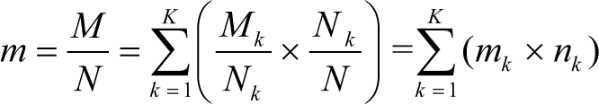
Assume there are R regions in the country, indexed r = 1, …, R, with 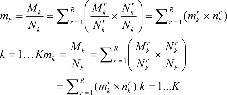
where
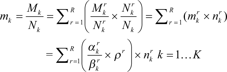
The GEA of group k(k = 1 … K) in region r, 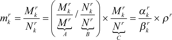
In Equation 3,
Substituting Equation 3 into Equation 2 yields the expression for the GEA of group k for the country in its entirety as:
Three forces will shape mk, the EA of persons from group k.
First, the distribution of the members of a group between the various regions. The greater the proportion of persons from the group living in regions with a high GEA (in other words,
As the GEA of a region (ρr) rises, so will the GEA of all the groups located within it. In other words, a rising tide will lift all boats.
Third, notwithstanding distribution shifts between regions, and changes in the GEA of regions, the GEA of a group will also depend upon community-specific factors or, as was termed earlier, its GP. This is reflected by the term
An Econometric Model of Educational Attainment
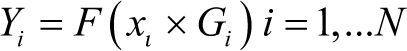
The relative strength of the various factors, set out in the previous section, on the likelihood of a person being a graduate or equivalent, can be analysed econometrically. The dependent variable Y defined over N young adults (persons 21–29 years of age) was assigned the value Yi = 1 if person i (i = 1 … N), was a graduate or equivalent and Yi = 0, if they were not. It was hypothesized that Y was a function of five determining variables—the person’s social group, sector (rural or urban), gender, household MPCE quintile, and region of residence—where, for each person, these last four variables were represented by the vector xi. The component
Furthermore, the social group variable, G, was defined as taking the value 1 (Gi = 1) if person i was from the ST, Gi = 2, if person i was from the SC, Gi = 3, if person i was from the OBC, Gi = 4, if person i was Muslim, and Gi = 5, if person i was from the FC. The econometric equation allowed each of the four components of the vector x—sector, gender, MPCE quintile and region—to interact with the social group variable, G, so that the equation estimated on observations for N persons was:
So, for example, since a person’s sector of residence was s in the vector x then, in Equation 5, the effect, on a person’s probability of being a graduate (or equivalent), of their living in a rural or urban area, ‘would be contingent on their social group’: living in a particular sector could have a differential effect on this probability, depending on whether the person was, say Muslim or from the FC. Within the context of this ‘interaction’ model, it is possible to test whether differences in the effect of a particular variable category (sector, gender, MPCE quintile, region), on the probability of being a graduate, were significantly different between the social groups.
Since the dependent variable (graduate/non-graduate), the estimated equation was binary, the model was formulated as a logit model. If 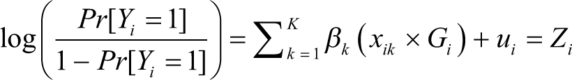
where: βk is the coefficient of variable k, k = 1 … K.
From Equation 6 it follows that:
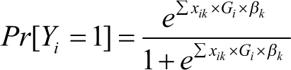
where the term ‘e’ in the above equation is the exponential term.
Predicted Probabilities
The results are presented in terms of ‘predicted probabilities’ (PP). These are described in Long and Freese (2014, Chapter 4) and in a Stata manual 10 and are based on the method of ‘recycled predictions’. Since they underpin the results of this article, their calculation and a brief description are contained below.
Suppose that one is interested in identifying the probability of a YA being a graduate which can be entirely ascribed to them being from the FC or from the SC. Note that simply computing the probabilities of GEA (using Equation 7) over the FC and SC subsamples would not provide this answer because the FC and SC subsamples would differ in more than just the caste of the individuals. These subsamples might differ in terms of sector, household resources, regional residence and so one could not attribute the subsample difference in probabilities of GEA solely to the ‘caste effect’.
To isolate the caste effect first treat all the YA in the data as belonging to the FC and then, apply the observed characteristic (sector, gender, household MPCE and region) values of the individuals in the sample to calculate the probability, using Equation 7, of GEA. Next, treat all the YA in the data as belonging to the SC and then apply the observed characteristic (sector, gender, household MPCE, region) values of the individuals in the sample to calculate the probability of GEA. The difference between the two sets of calculated probabilities of being a graduate is entirely the result of being from the FC or the SC because, in both calculations, the values of the characteristics used to compute these probabilities were identical. 11 Probabilities calculated using this methodology are PP.
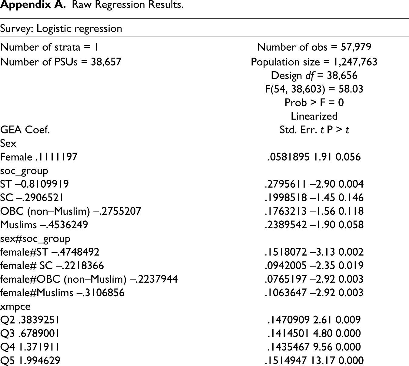
Estimation Results
Table 5 shows the results from estimating Equation 5. The equation was estimated on data for 57,979 YA drawn from the 21 major Indian states aggregated into five broad regions, as defined earlier, and shown in Table 5. The column labelled ‘Predicted Probability’ shows the PP, as defined above, of the various categories of variables. So, in terms of social groups, Table 5 shows that the PP of YA being graduates (or equivalent) was 14.3% for the ST, 18.5% for the SC, 21.8% for the OBC, 13.9% for Muslims, and 29.2% for the FC. As discussed above, these represent the ‘pure’ subgroup effect of GEA because they were computed with the values of the non-caste variables unchanged.
Predicted Probabilities of Educational Attainment by Social Group+.
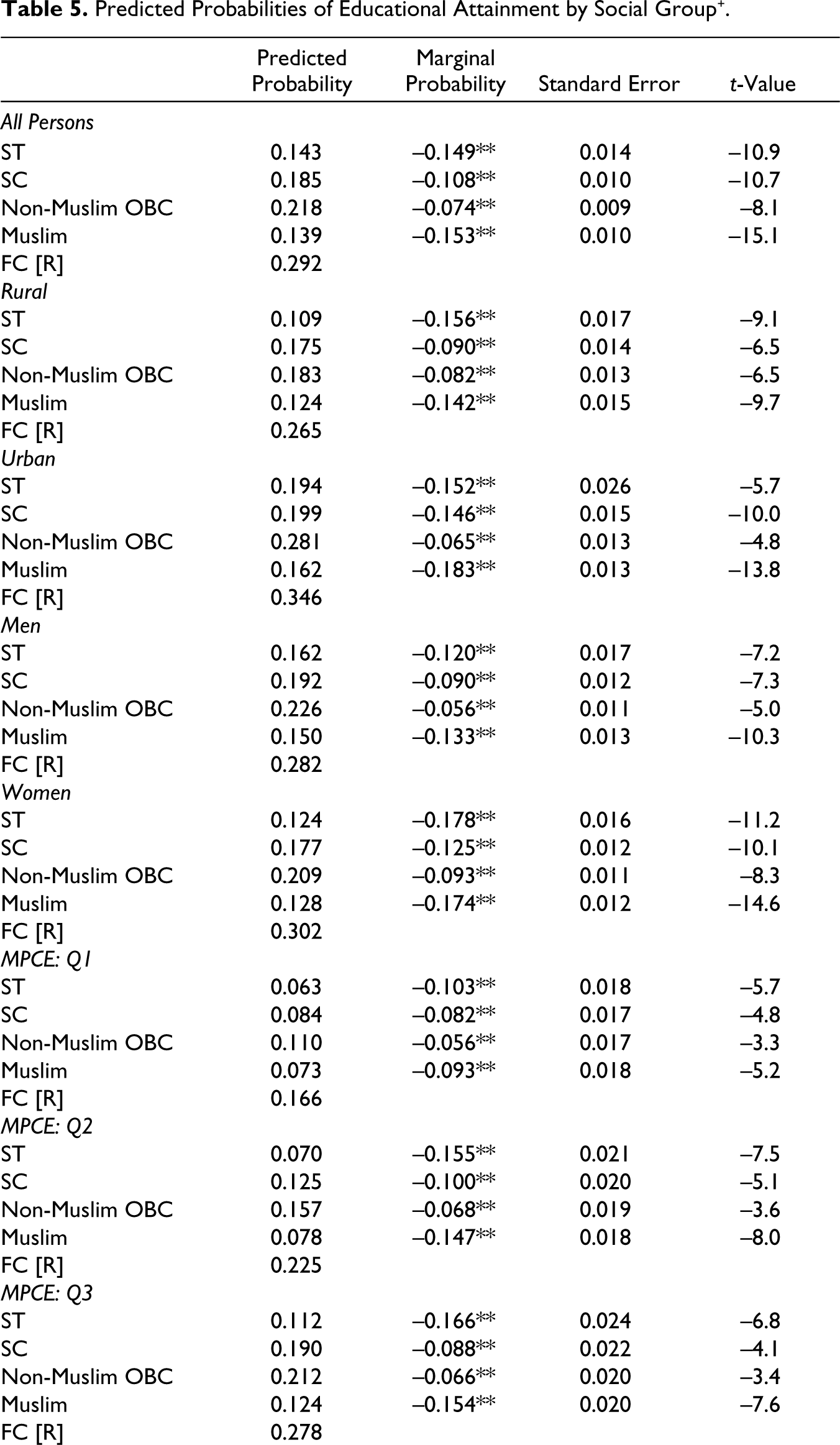
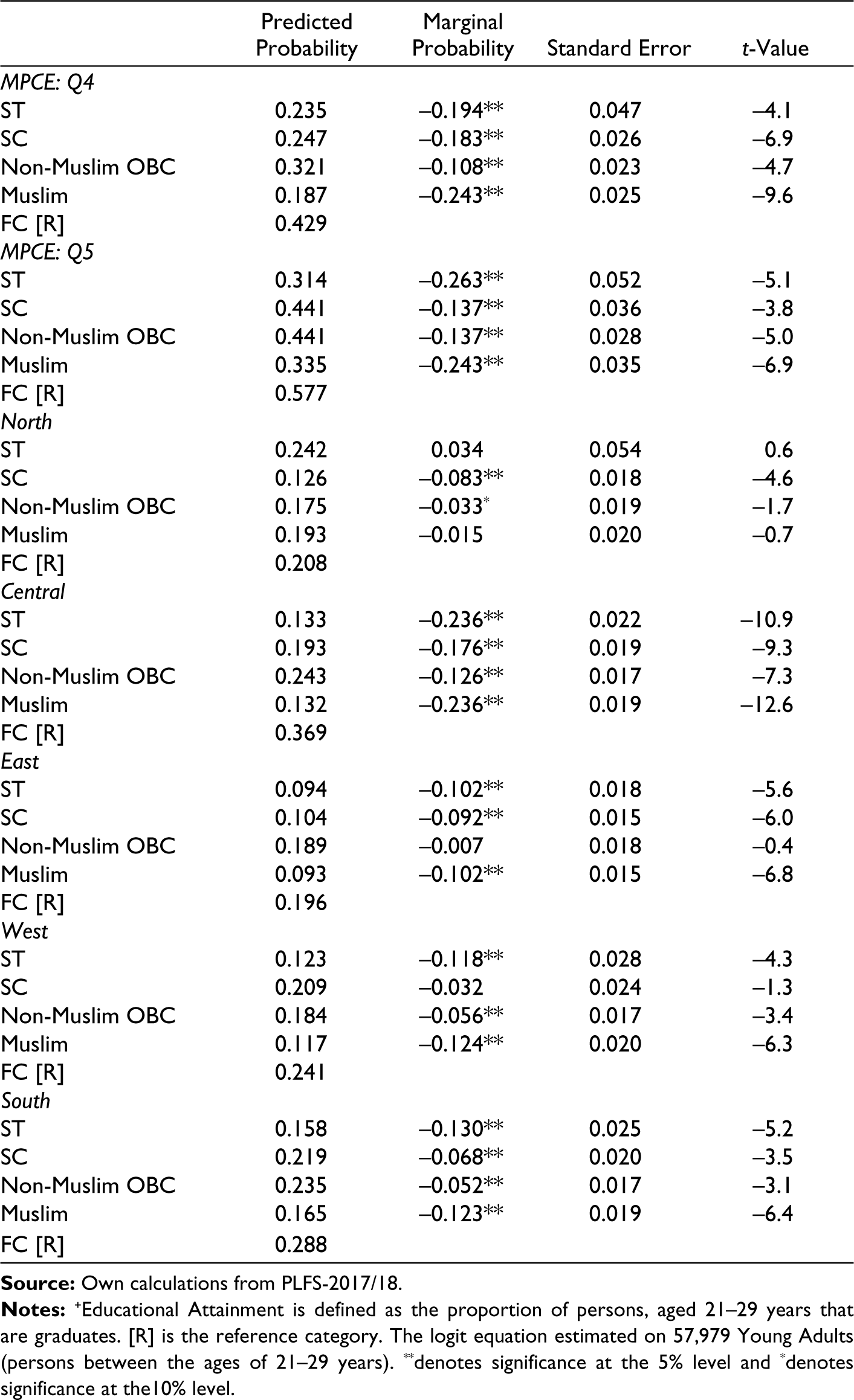
The column in Table 5 labelled ‘Marginal Probability’ represents, for the social group category, the differences between the PP of the individuals in the first four social groups and those in the reference group FC, denoted by [R]. Table 5 shows that the marginal probability for Muslims was –15.3 points (= 13.9 – 29.2) points. The ratios of these marginal probabilities and their standard errors (shown in the next column) are the t-values. These tested the null hypothesis that the marginal probabilities were zero.
Table 5’s first panel, labelled ‘All Persons’, shows that, compared to the non-FC groups, the PP of GEA of YA from the FC significantly higher. The statistical tests showed that, comparing between the non-FC groups, the difference between YA Muslims and those from the ST in their PP of GEA (14.3% and 13.9%, respectively) was not significant; however, the PP of GEA of YA Muslims was significantly lower than that for YA from the SC (18.5%); the PP of GEA for YA from the SC was significantly lower than that for YA from the OBC (21.8%). So, the econometric results make clear that, after neutralizing for non-social group factors, there was a clear hierarchy in terms of the PP of YA being graduates with those from the FC at the top, followed by the OBC, then by the SC, and with Muslims and the ST at the bottom.
Comparing Social Groups by Rural/Urban Sector
The next panels of Table 5 compare the PP of the social groups for specific categories of the determining variables. The panels labelled ‘Rural’ and ‘Urban’ shows the PP of GEA of YA men and women from the five social groups, respectively. Once again, the finding was that after neutralizing for non-group factors, there was a hierarchy in terms of the PP of both rural and urban YA being graduates with those from the FC at the top, followed by the OBC, then by the SC, and with Muslims and the ST at the bottom.
A feature of interest about the estimation results is that for YA from every social group, the PP of GEA was greater for urban than for rural residents. Thus, for example, the PP of GEA of YA from the FC was significantly larger if they were in urban (34.6%) than in rural (26.5%) areas. Overall, the PP of GEA of urban YA (25.3%) was significantly larger than that for rural YA (18.4%).
Comparing Social Groups by Gender
The next two panels of Table 5 compare the PP of the social groups for specific categories of the determining variables. The panels labelled ‘Men’ and ‘Women’ shows the PP of GEA of YA men and women from the five social groups, respectively. Once again, the finding was that, after neutralizing for non-group factors, there was a clear hierarchy in terms of the PP of YA men and women being graduates with those from the FC at the top, followed by the OBC, then by the SC, and with Muslims and the ST at the bottom.
Comparing the panels for men and women, the statistical tests showed that the PP of GEA was higher for male, compared to female, YA from the ST (16.2% versus 12.4%), the OBC (22.6% versus 20.9%) and Muslims (15% versus 12.8%). However, there did not appear to be any significant difference, in the PP of GEA, between male and female YA from the SC (19.2% and 17.7%) and between male and female YA from the FC (28.2% and 30.2%). 12 Overall, the PP of GEA of male YA (21.4%) was significantly larger than that for female YA (20.5%).
Comparing Social Groups by Household MPCE
The five panels in Table 5, headed ‘MPCE: Q1’–‘MPCE: Q5’, show the PP of GEA by social group for each of the five quintiles of household MPCE ranging from the lowest (Q1) to the highest (Q5) quintile. The results clearly showed that the PP of GEA for YA from every social group rose as their household MPCE improved. For FC households in the lowest quintile of MPCE, the PP of their YA being graduates (or equivalent) was 16.6%, and this rose to 57.7% for FC households were in the highest quintile of MPCE. At the other end of the spectrum, for ST and Muslim and households in the lowest quintile of MPCE, the PP of their YA being graduates (or equivalent) was 6.3% and 8.4%, respectively, and these probabilities rose to 31.4% and 33.5% for ST and Muslim households in the highest quintile of MPCE. Overall, the PP of GEA of young adults with households in the various quintiles of MPCE was 10.4% (Q1), 14.3% (Q2), 19.7% (Q3), 29.7% (Q4) and 43.7% (Q5).
Notwithstanding the positive association, for every social group, between household resources and the probability of YA being graduates it remained the case that, in every quintile of household resources, there was an identical hierarchy to that noted earlier: After neutralizing for non-group factors, the highest PP of GEA for young adults was for the FC and lowest was for Muslims and the ST. In terms of disadvantaged groups, the results in Table 5 make clear that the PP of GEA of Muslim YA was inferior to that of their SC counterparts.
Comparing Non-FC Social Groups by Household MPCE
The preceding subsection showed that households’ resources (as proxied by their MPCE) were an important determinant of the PP of their YA being graduates (or equivalent). This subsection asks whether the same level of household resources affected the PP of GEA differently for YA from the different social groups.
The PP of Muslims and SC young adults being graduates (or equivalent), in the lowest quintile of household MPCE, was 7.3 and 8.4%, respectively, and this difference was not statistically significant. If we regard households in the lowest quintile of MPCE as being ‘poor’, the PP of GEA of YA Muslims and YA from the SC from poor households was (statistically) identical. In addition, for YA from poor households, the PP (of GEA) of YA from the ST (6.3%), the SC (8.4%) and Muslims (7.3%) was not statistically significant. For poor households, however, compared to the other non-FC groups, the PP (of GEA) of YA from the OBC (11%) was significantly higher.
As household resources improved, lifting them out of poverty, a significant gap emerged between SC and Muslim YA in their PP of GEA: for Q2, it was 12.5% versus 7.8%; for Q3, it was 19% versus 12.4%; for Q4, it was 24.7% versus 18.7%; and, for the highest quintile, it was 44.1% versus 33.5%. This suggests that YA from SC and Muslim ‘non-poor’ households had different attitudes towards the importance of being a graduate. This raises the question of why non-poor YA from two disadvantaged groups, SC and Muslim, should value graduate qualifications differently.
Muslims had an advantage over the SC in that they were, to a greater extent than the SC, located in urban areas: Aaccording to PLFS-2017/18, 41% of Muslim YA lived in urban areas, in contrast to 25% of YA from the SC. On the face of it, this should have provided Muslim YA greater opportunities for higher education than their counterparts in the SC. However, as Gaynor and Jaffrelot (2011) have pointed out, in their detailed ethnographic study of urban Muslims in India, that Muslims are marginalized in Indian cities. In the former princely states, such as Bhopal and Hyderabad, the end of aristocracy has meant a loss of patronage for artisans and the loss of Urdu as an official language has hastened the decline. Muslim enclaves in other parts of India are located away from the city’s core and are characterized by low levels of public service provision. So, all in all, urbanization does not deliver to Muslims the advantages that one might expect from living in an urban environment.
Discrimination and Attitudes Towards Education
Both Muslims and the SC face discrimination: Muslims on the grounds of religion and the SC on the grounds of untouchability. The difficulties that Muslims and persons from the SC faced in renting houses in five metropolitan areas of the National Capital Region of Delhi were detailed in Thorat et al. (2015). House owner prejudices meant that they were either denied tenancy, or, if they were granted tenancy, it was on unfavourable terms and with conditions attached. Similarly, Thorat and Attewell (2010) showed that college-educated Muslims and persons from the SC, when applying for jobs, did less well than equivalently qualified high caste persons. Their findings suggest that ‘caste favouritism’ and the social exclusion of Muslims and SC persons occurred even in the most dynamic sectors of the Indian economy.
‘Stereotype threat’ refers to the phenomenon whereby persistent discrimination reduces the confidence of victims (of discrimination) and undermines their self-esteem because they begin to believe that they are of low worth. Consequently, negative stereotypes-based discrimination—referred to by Bertrand et al. (2005) as ‘implicit discrimination’—erodes people’s motivation for equipping themselves for advancement.
Jeffery and Jeffery (1997) in their study of Muslims in Bijnor argued that many Muslims regarded their relative economic weakness as stemming from their being excluded from jobs due to discriminatory practices in hiring. The belief that their sons would not get jobs then led Muslim parents to devalue the importance of education as an instrument of upward economic mobility. It was with such considerations in mind that Myrdal (1944) spoke of the ‘vicious circles of cumulative causation’: The failure of discriminated groups to make progress justifies the prejudicial attitudes of dominant groups.
While it is also the case that the SC face discrimination in education and employment (Thorat & Newman, 2010), they are, unlike Muslims, the beneficiaries of India’s ‘reservation’ policies. Post-independence India adopted a constitution which made special provisions for its ‘backward castes’. Reservation policies established quotas in representative politics: the national parliament, state legislatures, municipality boards and village councils (panchayats). Quotas were established for government jobs and jobs in publicly funded (or publicly assisted) organizations and for places in public higher educational institutions. It was Dalits and the ST that benefited from these policies which reserved 23% of jobs and higher education places for them. Then, in 1990, a further 27% was reserved for the OBC. Thus, apart from Muslims, all the non-FC groups in India benefit from ‘reservation policies’.
Since reservation benefits in India are based on caste and not on religion, Muslims have not gained from them. Consequently, Muslims from the OBC—approximately 40% of India’s Muslims—are entitled to reservation benefits by virtue of belonging to a OBC if their group is officially recognized as an OBC. 13 Since this recognition is the responsibility of states, reservation benefits for Muslims vary from state to state. Consequently, Muslim YA, who do not have the protection of reservation policies, have less the incentive to acquire qualifications than their counterparts from the SC. 14
Comparison of the GEA of the Social Groups in the Different Regions
Table 5 also identifies the regions where the groups did badly in terms of GEA PP. Muslims did best in the North (mainly because of Jammu and Kashmir) with a PP of 19.3%, and they did worst in the East (PP of 9.3%). The ST fared worst in the East (PP of 9.4%) and best in the North (mainly because of Uttarakhand) with a PP of 24.2%. The SC fared worst in the East and in the North (with PP of 10.4% and 12.6%, respectively) and did best in the Southern and Western regions (with PP of 20.9% and 21.9%, respectively).
One can also compare the PP of YA being graduates (or equivalent), across the 21 states which aggregate into the five broad regions listed in Table 5. Using Tamil Nadu as the reference (or comparator state), shows that the social groups’ marginal probabilities were mostly negative, meaning that the PP of GEA of young adults was, in 19 of the 21 states, smaller than (the 26.6%) in Tamil Nadu. 15 In the case of 16 of these 19 states, the difference was significantly different from zero. It would not be farfetched to say, therefore, that in terms of the GEA of young adults in India, Tamil Nadu leads the way.
Endowments Versus Coefficients in Explaining Graduate Educational Achievement
Table 2 noted that the difference in the observed proportion (OP) of FC and SC young adult graduates was 18.5 percentage points (34.3% and 15.8%, respectively). This difference can be ascribed to two causes: (a) because of differences between the groups in the observed values of their explanatory variables and (b) because of differences between the groups in their estimated coefficients. These two causes may be termed the ‘endowment’ and the ‘coefficient’ effects, respectively. The purpose of this section is to determine the size of these two effects in explaining the observed difference in the proportion of YA that are graduates (or equivalent) between each of the non-FC groups and the FC.
The fourth section differentiated between the OP and the PP of GEA for YA in each social group. Denote the social groups’ OP as
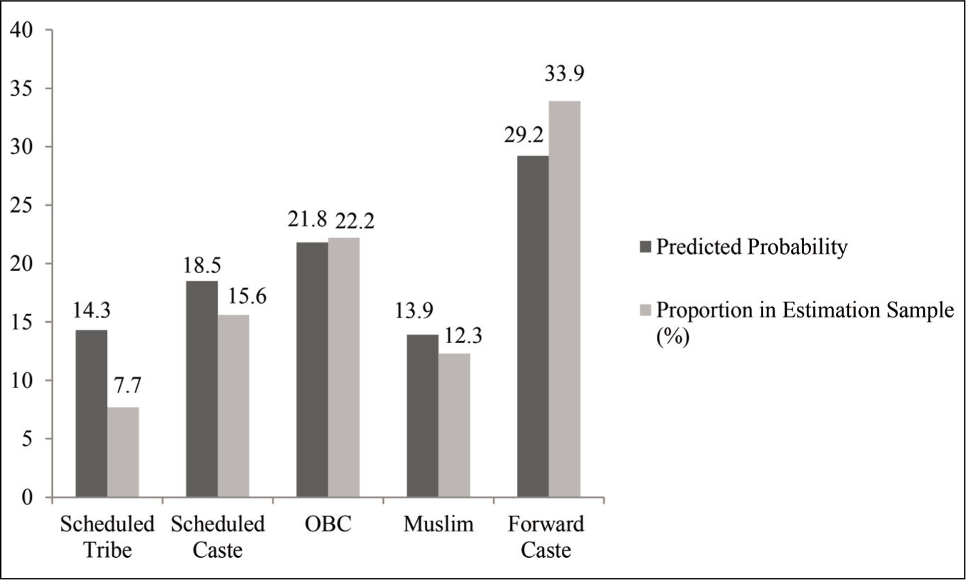
Figure 1 shows that for three groups—ST, SC and Muslims—the OP of GEA (7.7%, 15.6% and 12.3%, respectively) was less than their corresponding PP. This means that their group’s GEA-related endowments were inferior to that of the sample in its entirety. For the FC, the OP of GEA was greater than the PP: This means that FC GEA-related endowments were superior to that of the sample in its entirety. For the OBC, the OP of GEA was almost the same as its PP (22.2% versus 21.8%): This means that OBC GEA-related endowments were the same as that of the sample in its entirety.
Consequently, it is possible to decompose the difference in OP between two groups, say FC and Muslim (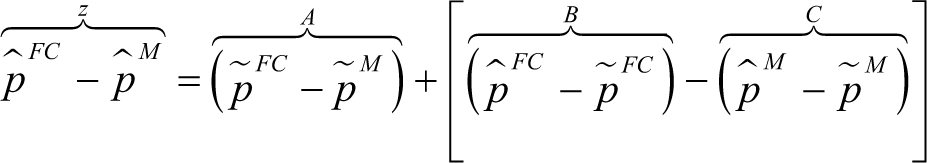
The term Z > 0 if, by assumption,
In Equation 8, the term B and C are the difference for, respectively, the FC and Muslims between their OP and PP of GEA. Therefore, they represent, the relative superiority (B, C > 0) or inferiority (B, C < 0) of the group’s endowments over the general level of endowments of social groups considered in their entirety. 16 The difference between the two terms B and C in Equation 8 is a measure of the ‘relative’ superiority, (B – C) > 0/inferiority (B – C) < 0 of the attributes of YA from the FC vis-à-vis their Muslim counterparts.
The term A > 0 and (B – C) > 0. Then the ‘graduate propensities’ of FC young adults are superior to that of Muslims (δ > 0), and they also have superior endowments (λ > 0). A > 0 and (B – C) < 0. Then Z > 0 despite the relative ‘inferiority’ of FC to Muslim endowments (λ < 0) because the graduate propensities of FC young adults is superior to that of Muslims. A <0 and (B – C) > 0. Then Z > 0 despite the superior GP of Muslim young adults because the relative endowment superiority of FC young adults endowments (λ > 0) outweighs this.
In Equation 8, B and C could be positive or negative. If, say, C < 0, then
The empirical results corresponding to Equation 8 are shown in Table 6. Differences in the OP of graduate YA from the FC and those from the other groups (ST, SC, OBC and Muslims, respectively) were 26.2, 18.3, 11.7 and 21.6 percentage points. The corresponding differences in the PP of young adults from the FC and those from the other groups (the ST, SC, OBC and Muslims, respectively) were much smaller: 14.9, 10.7, 7.4 and 15.3 percentage points.
Propensity versus Characteristics in GEA by Social Group.
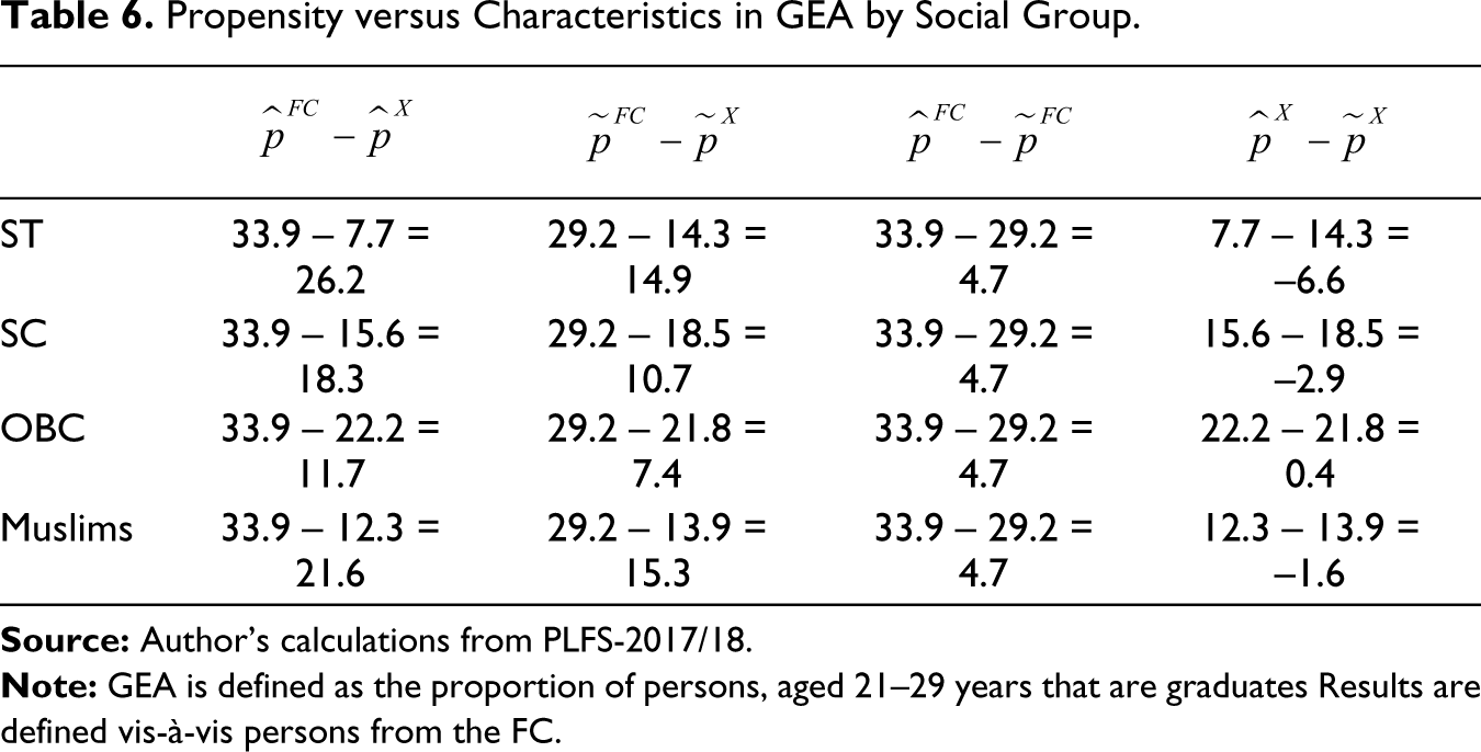
Remembering that PP gaps represent GP differences between the non-FC groups and the FC, the largest propensity difference related to Muslims: 70.8% (=15.3/21.6) of the FC-Muslim OP gap in the GEA of their young adults were due to differences in propensity. The smallest propensity difference was between the SC and the ST: 58.5% (=10.7/18.3) of the FC-SC OP gap and 56.9% (=14.9/26.2) of the FC-ST OP gap, in the GEA of their young adults was due to propensity difference. The corresponding figures for YA from the OBC was 63.2% (=7.4/11.7).
Poverty as a Barrier to Educational Attainment
The link between lack of resources and educational attainment is brought out very clearly in Table 3: Only 9% YA whose households were in the first quintile of MPCE—compared to 52.9% of those in households in the top quintile—were graduates or (equivalent). Since nearly half of YA from the ST (48.8%), and over a third of YA from the SC (34.5%), belonged to households in the lowest quintile of MPCE, it might be thought that this fact alone—quite apart from any group-based propensity to be graduates—would inhibit GEA. So, the question is to what extent would the educational attainment of the non-FC groups be improved if they had more economic resources?
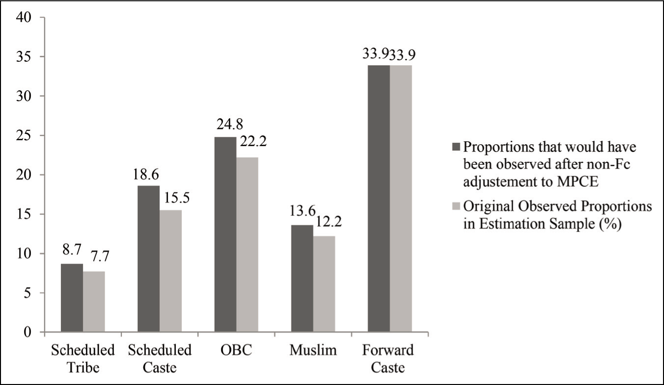
To answer this question, a simulation was conducted in which all non-FC households in the lowest quintile of MPCE were raised to the next (Q2) quintile and all non-FC households in the second quintile of MPCE were raised to the next (Q3) quintile. These new values were used in the logit equation to re-compute what would now be the new OP:
Figure 2 compares the original PP of group EA (i.e., the sample proportions) with the new PP. This shows that under their new affluence, the proportion of graduates among YA would rise from 7.7% to 8.7% for the ST, 15.5% to 18.6% for the SC, 22.2% to 24.8% for the OBC, and 12.2% to 13.6% for Muslims. There was, of course, no change for the FC since its household MPCE quintiles had not been altered.
Conclusions
This article argued that the low educational attainment—defined as the proportion of YA (persons aged 21–29-year-olds) that are graduates—of non-FC groups vis-à-vis the FC was partly due to the lower propensity of persons from the non-FC for graduate-level education and partly to a less favourable configuration of education-friendly endowments. An important endowment was rural/urban location of YA; another was the MPCE of the YA’s households; a third was the broad region (arrived at by a grouping of Indian states) in which the YA lived.
Educational attainment defined in terms of the proportion of YA in a community that are graduates is but one facet of the educational achievement of a community. Other, arguably equally important aspects, are first, the proportion of a community’s 15–24-year-olds that are enrolled in educational institutions and, second, the proportion of this group that are not in NEET. Although these aspects are not studied in this article, they deserve serious analysis in future work.
In conducting its analysis, the article painted a ‘stylized’ picture of GEA in India, omitting some details, but focusing on what it believed are the essentials. Other studies of GEA might focus on details but, for that reason, fail to do justice to an all-India scenario. So, while acknowledging that the article might not include details which an ethnographic observer thought important, its merit is that by presenting a parsimonious model which captures the essence of the GEA problem, it does not miss the wood for the trees.
Footnotes
Acknowledgements
I am grateful to the Editor and to three anonymous referees for comments that have greatly improved this article.
Declaration of Conflicting Interests
The author declared no potential conflicts of interest with respect to the research, authorship, and/or publication of this article.
Funding
The author received no financial support for the research, authorship, and/or publication of this article.
Raw Regression Results.
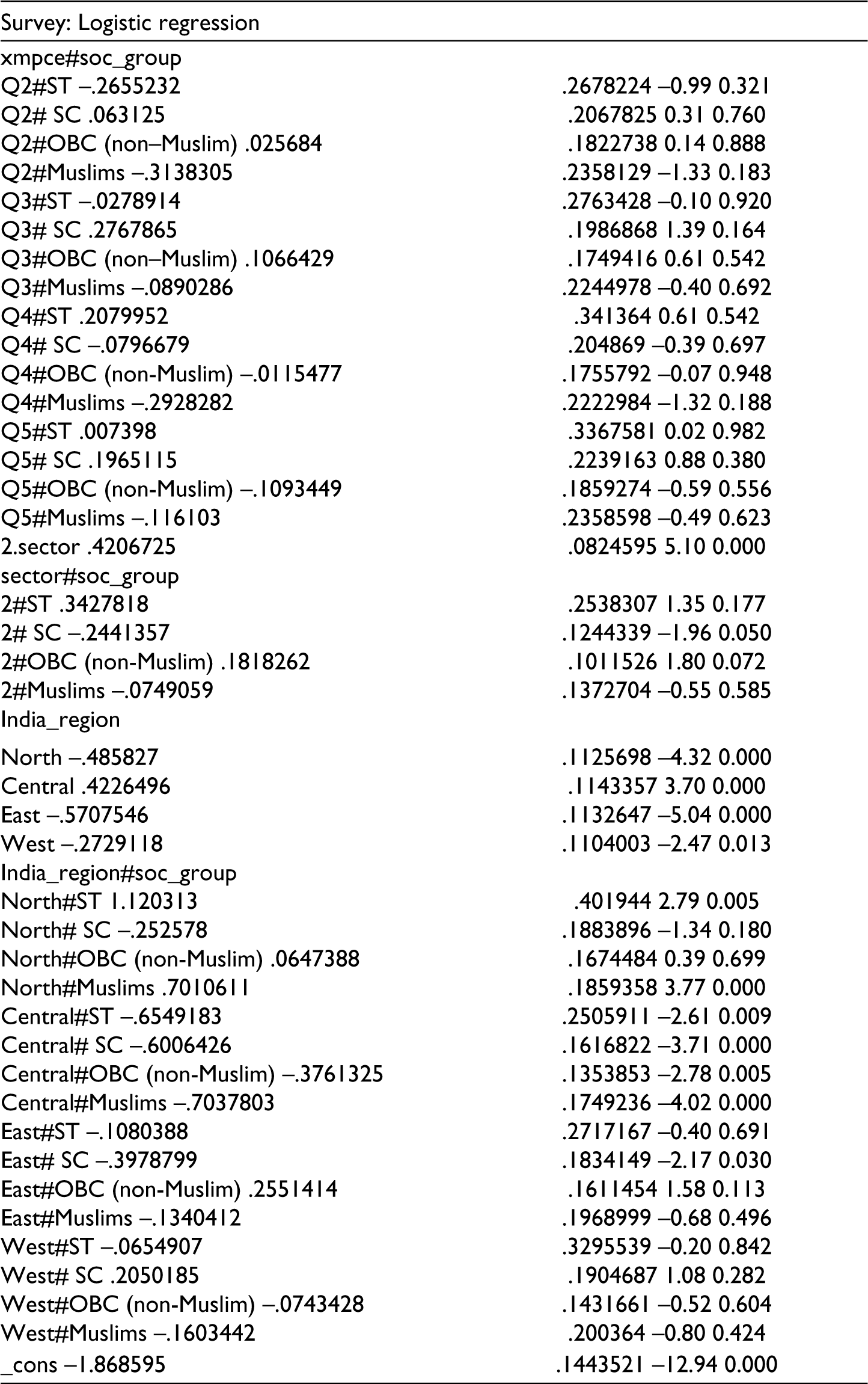
| Survey: Logistic regression | |
| Number of strata = 1 | Number of obs = 57,979 |
| Number of PSUs = 38,657 | Population size = 1,247,763 |
| Design df = 38,656 | |
| F(54, 38,603) = 58.03 | |
| Prob > F = 0 | |
| Linearized | |
| GEA Coef. | Std. Err. t P > t |
| Sex | |
| Female .1111197 | .0581895 1.91 0.056 |
| soc_group | |
| ST –0.8109919 | .2795611 –2.90 0.004 |
| SC –.2906521 | .1998518 –1.45 0.146 |
| OBC (non–Muslim) –.2755207 | .1763213 –1.56 0.118 |
| Muslims –.4536249 | .2389542 –1.90 0.058 |
| sex#soc_group | |
| female#ST –.4748492 | .1518072 –3.13 0.002 |
| female# SC –.2218366 | .0942005 –2.35 0.019 |
| female#OBC (non–Muslim) –.2237944 | .0765197 –2.92 0.003 |
| female#Muslims –.3106856 | .1063647 –2.92 0.003 |
| xmpce | |
| Q2 .3839251 | .1470909 2.61 0.009 |
| Q3 .6789001 | .1414501 4.80 0.000 |
| Q4 1.371911 | .1435467 9.56 0.000 |
| Q5 1.994629 | .1514947 13.17 0.000 |
| xmpce#soc_group | |
| Q2#ST –.2655232 | .2678224 –0.99 0.321 |
| Q2# SC .063125 | .2067825 0.31 0.760 |
| Q2#OBC (non–Muslim) .025684 | .1822738 0.14 0.888 |
| Q2#Muslims –.3138305 | .2358129 –1.33 0.183 |
| Q3#ST –.0278914 | .2763428 –0.10 0.920 |
| Q3# SC .2767865 | .1986868 1.39 0.164 |
| Q3#OBC (non–Muslim) .1066429 | .1749416 0.61 0.542 |
| Q3#Muslims –.0890286 | .2244978 –0.40 0.692 |
| Q4#ST .2079952 | .341364 0.61 0.542 |
| Q4# SC –.0796679 | .204869 –0.39 0.697 |
| Q4#OBC (non-Muslim) –.0115477 | .1755792 –0.07 0.948 |
| Q4#Muslims –.2928282 | .2222984 –1.32 0.188 |
| Q5#ST .007398 | .3367581 0.02 0.982 |
| Q5# SC .1965115 | .2239163 0.88 0.380 |
| Q5#OBC (non-Muslim) –.1093449 | .1859274 –0.59 0.556 |
| Q5#Muslims –.116103 | .2358598 –0.49 0.623 |
| 2.sector .4206725 | .0824595 5.10 0.000 |
| sector#soc_group | |
| 2#ST .3427818 | .2538307 1.35 0.177 |
| 2# SC –.2441357 | .1244339 –1.96 0.050 |
| 2#OBC (non-Muslim) .1818262 | .1011526 1.80 0.072 |
| 2#Muslims –.0749059 | .1372704 –0.55 0.585 |
| India_region | |
| North –.485827 | .1125698 –4.32 0.000 |
| Central .4226496 | .1143357 3.70 0.000 |
| East –.5707546 | .1132647 –5.04 0.000 |
| West –.2729118 | .1104003 –2.47 0.013 |
| India_region#soc_group | |
| North#ST 1.120313 | .401944 2.79 0.005 |
| North# SC –.252578 | .1883896 –1.34 0.180 |
| North#OBC (non-Muslim) .0647388 | .1674484 0.39 0.699 |
| North#Muslims .7010611 | .1859358 3.77 0.000 |
| Central#ST –.6549183 | .2505911 –2.61 0.009 |
| Central# SC –.6006426 | .1616822 –3.71 0.000 |
| Central#OBC (non-Muslim) –.3761325 | .1353853 –2.78 0.005 |
| Central#Muslims –.7037803 | .1749236 –4.02 0.000 |
| East#ST –.1080388 | .2717167 –0.40 0.691 |
| East# SC –.3978799 | .1834149 –2.17 0.030 |
| East#OBC (non-Muslim) .2551414 | .1611454 1.58 0.113 |
| East#Muslims –.1340412 | .1968999 –0.68 0.496 |
| West#ST –.0654907 | .3295539 –0.20 0.842 |
| West# SC .2050185 | .1904687 1.08 0.282 |
| West#OBC (non-Muslim) –.0743428 | .1431661 –0.52 0.604 |
| West#Muslims –.1603442 | .200364 –0.80 0.424 |
| _cons –1.868595 | .1443521 –12.94 0.000 |
Social Groups in India
The caste system in India stratifies Hindus, constituting 80% of the population, into mutually exclusive groups, membership of which is determined entirely by birth, with the caste into which a person is born playing an important role in determining their life prospects. Very broadly, one can think of the FC as comprising the three subgroups: Brahmins, Kshatriyas and Vaisyas. (These three castes are said to have come from Brahma’s mouth [Brahmin], arms [Kshatriya] and thighs [Bania]. This is termed the Purusasukta legend which appears in an appendix to the Rig Veda.)
Below these are the non-FC. These comprise, first, the OBC, who, while included in the Hindu caste system as its fourth caste, traditionally performs menial jobs. Then there are those persons (mostly Hindu, but some who have converted to Buddhism or Christianity) with whom the four castes, delineated above, regard any physical contact as polluting or unclean: This is the practice of ‘untouchability’. They are separately identified and referred to in this paper as the SC. Also identified separately are the ST. There are about 85 million Indians classified as belonging to the ST. Of these, Adivasis (meaning original inhabitants) refer to the 70 million who live in Central India, in a relatively contiguous hill and forest belt extending across the states of Gujarat, Rajasthan, Maharashtra, Madhya Pradesh, Chhattisgarh, Jharkhand, Andhra Pradesh, Orissa, Bihar and West Bengal (Guha, 2007).
The last group of persons are Muslims who, in terms of religion, bear the brunt of deprivation and exclusion in India. The Sachar Committee (2006) in its report to the government of India highlighted the backwardness of Indian Muslims. This Report drew attention to a number of areas of disadvantage, inter alia, the existence of Muslim ghettos stemming from their concern with physical security, low levels of education engendered by the poor quality of education provided by schools in Muslim areas, pessimism that education would lead to employment, difficulty in getting credit from banks, and the poor quality of public services in Muslim areas. Basant and Shariff (2010), Basant (2013) and Kabir (2019) provide further analysis of the educational and economic conditions of Muslims.