COVID-19 Lifecycle: Predictive Modelling of States in India

Abstract

The study captures the COVID-19 lifecycle in different states of India using predictive analytics. Drawing upon the seminal susceptible–infected–removed (SIR) model of capturing the spread of viral diseases, this study models the spread of COVID-19 in the ten most infected states of India (as on 30 April 2020). Using publicly available state-wise time series data of COVID-19 patients during the period 1–30 April 2020, the study uses the forecasting technique of auto-regressive integrated moving averages (ARIMA) to predict the likely population susceptible to COVID-19 in each state. Thereafter, based on the SIR model, predictive modelling of state-wise COVID-19 data is carried out to determine: (a) the predictive accuracy; (b) the likely number of days it would take for the disease to reach the peak number of infections in a state; (c) the likely number of infections at the peak; and (d) the state-wise end date. The SIR model is implemented by running Python 3.7.4 on Jupyter Notebook and using the package Matplotlib 3.2.1 for visualization. The study offers rich insights for policymakers as well as common citizens.

Keywords

COVID-19 India SIR model predictive analytics ARIMA

Introduction

The COVID-19 pandemic has probably been the most influential public catastrophe encountered by humankind since World War II. It has changed our outlook towards life and its existential uncertainty. It has forced us to adopt a lifestyle which is different from the one we are used to. It has put a question mark over our economic survival. And even as it has given us an opportunity to reflect and introspect, learn, unlearn and relearn, it still is a nemesis. Therefore, it is but natural to explore its lifecycle patterns. A cautious endeavour to capture the uncertainty may help in planning without displaying over-optimism or undue pessimism about the future. A data-driven approach to predict the COVID-19 lifecycle, based on robust theoretical framework in extant research related to viral infections, may give us greater insights and help us to prepare rationally for the challenges that lie ahead.

Even as researchers the world over are trying to capture the COVID-19 infection data and build predictive models, to the best of our knowledge, no such attempt has been made in India so far. Moreover, no study so far has attempted to do predictive modelling at a comparatively granular level of each state in India. Such a study is relevant at two levels. First, India offers a unique set-up for the spread of infectious diseases. While we have a robust universal vaccination programme (Banik et al., 2020) and a proven track record of completely eliminating various viral diseases, we are also hampered by a large population and high population density. Second, in a federal structure, different states in India have been able to implement various policies to prevent the spread of COVID-19 with different levels of efficacy. This has resulted in extremely different rates of spread of the disease in different states of India. Therefore, the very specific objective of this study is to carry out predictive modelling of the COVID-19 lifecycle pattern of various states in India. In the process, the study determines: (a) the predictive accuracy; (b) the likely number of days it would take for the disease to reach the peak number of infections in a state; (c) the likely number of infections at the peak; and (d) the state-wise end date. The rest of the article is structured as follows: the second section lays down the conceptual framework; the third section gives a description of the research method; the fourth section presents results from the study; and, finally, the fifth section offers a discussion on implications.

Conceptual Framework

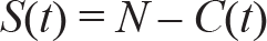
The study is based on the susceptible–infected–removed (SIR) model (Kermack & McKendric, 1927) of viral infection. The model divides the population into three categories: susceptible, infected and removed. The SIR model has been used by various studies in the recent past to model the spread of COVID-19 (e.g., Liu et al., 2020) and also for other infectious diseases, in general (Bhattacharya et al., 2015; Muthuramakrishnan & Martin, 2016). The SIR model captures incremental changes in the number of susceptible, infected and removed individuals over a period of time in a region and, therefore, is summed up in terms of the following three equations:

d s / d t = - β (s i)

d i / d t = β (s i) - v^{'} (i)

d r / d t = v^{'} (i)

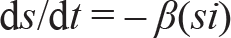
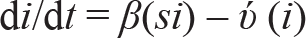
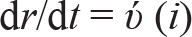
where s = S/N, i = I/N, and r = R/N. The various variables, parameters and their respective acronyms in the SIR model are as follows:

1. N: The population. It need not be equal to the population of the state. It is the population of people who may get affected by the disease.

N = S (1),

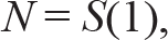
wherein S(1) gives the susceptible population at the beginning of the time period.

2. S(t): Number of individuals in the society who are susceptible to the disease at time t. This number is unknown and can safely be assumed to be equal to N at the beginning of the time period. These individuals are not yet infected.

S (t) = N - C (t)

3. C(t): The number of cases reported at time t. It should be equal to the total number of individuals infected and removed (quarantined for treatment).

C (t) = I (t) + R (t)

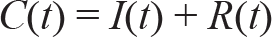
4. I(t): The number of individuals infected at time t. They are capable of transmitting the disease to those who are still in the susceptible category.

5. R(t): The number of individuals removed up to time t. The individuals belonging to this category can neither be infected again nor infect others.

6. R₀: The reproductive number.

7. β: The effective contact rate.

8. ύ: The removal rate. It is the inverse of the expected duration of infection.

The SIR model captures two directions of movement—from susceptible to infected and from infected to removed (Bhattacharya et al., 2015). Further, the SIR model is based on the following assumptions:

The population size, N, is constant.

The contact and removal rates are constant.

There are no demographic changes during the period of assessment.

The population is well-mixed such that any infected individual has a probability of contacting any susceptible individual.

The possible variants of the SIR model that can provide a theoretical framework for modelling the spread of an epidemic are the susceptible–exposed–infectious–recovered (SEIR) and susceptible–infected–recovered–deceased (SIRD) models. The SEIR model assumes that the virus incubates inside the host for a period of time before the infected individual becomes infectious and is, therefore, more suitable for those epidemics having a significant incubation period (Li et al., 1999). The SIRD model, on the other hand, considers recovered and deceased as separate compartments and, therefore, has to take into consideration the mortality rate. Some of the recent research has attempted to model COVID-19 using the SIRD model (e.g., Caccavo, 2020). A major prerequisite for modelling an epidemic using the SEIR or SIRD model is having to consider the possible incubation period of virus and mortality rate per unit time, respectively. Given the fact that research is still in progress on various aspects of COVID-19, there is a great degree of uncertainty regarding these values. For example, Fernández-Villaverde and Jones (2020) model COVID-19 using the SIRD model, considering a mortality rate of 0.8 per cent but with the caveat that ‘there is substantial uncertainty about this number’. Since the research on COVID-19 is still in its infancy, the authors of the present study use the SIR model to avoid having to adopt additional assumptions related to the incubation period or the mortality rate. However, once more information is available, the authors intend to use the SIRD framework for modelling COVID-19 in future studies.

Research Design

Data

The data for the study was obtained from publicly available sources (Rajkumar, 2020). Even as the dataset has data from the beginning of the outbreak of COVID-19 in a given state, we considered data during 1–30 April 2020. This was done to catch the trend of infection in the general public rather than capture sporadic noise in the data.

Methodology

The following parameters were calculated as follows:

Susceptible population at the beginning (N)

Time series regression analysis technique of auto regressive integrated moving average (ARIMA) is used for estimating N or the initially susceptible population. This is based on the usage of a similar method to estimate N in the extant literature on COVID-19 modelling (Batista, 2020). Data was analysed state-wise. The autocorrelation function (ACF) and partial autocorrelation function (PACF) values suggest there is no seasonality in the data. A good fit was observed between actual and predicted values for the available data points (1–30 April 2020). ARIMA was conducted to forecast the number of cases 60 days ahead [C(90)]. This is based on the assumption that out of all the people living in a state, all the susceptible cases would be exposed within 3 months from the start date of current time series (1 April 2020) and within 5 months from the confirmation of the first case in India. The first case in India was confirmed on 31 January 2020 in Kerala. It is a conservative estimation, since predicting too far ahead beyond the currently available data (30 days: 1–30 April 2020) at a time when there is still uncertainty in data capturing may lead to an erroneous forecast.

The basic reproduction number (R ₀ )

The basic reproduction number, R_0, is defined as the expected number of secondary cases produced by a single (typical) infection in a completely susceptible population (Jones, 2007). It is one of the most critical values which influences the rate of spread. Since the beginning of COVID-19, a number of studies have attempted to determine the value of R₀. Unfortunately, there is huge variance between the numbers suggested by various studies, with the World Health Organization (WHO)–recommended figure being at the lower end of the spectrum. Liu et al. (2020) summarized the findings from 12 studies on COVID-19 conducted during 1 January to 7 February 2020 to conclude that the estimates for R₀ ‘ranged from 1.4 to 6.49, with a mean of 3.28, a median of 2.79 and interquartile range (IQR) of 1.16’ (p. 1). For this study, we have taken the value of R₀ to be 3.28, as recommended by Liu et al. (2000). This value suggests that every infected individual, during every single day of non-confirmation, infects a little more than three other susceptible individuals in the population. Considering the R₀ value as 3.28 might seem negatively biased for a dense country like India, and assuming the same value of R₀ for all the states may look like a simplistic assumption. However, as more data is accumulated post-lockdown, the estimation error for R₀ is likely to decrease and a clearer state-wise picture could emerge.

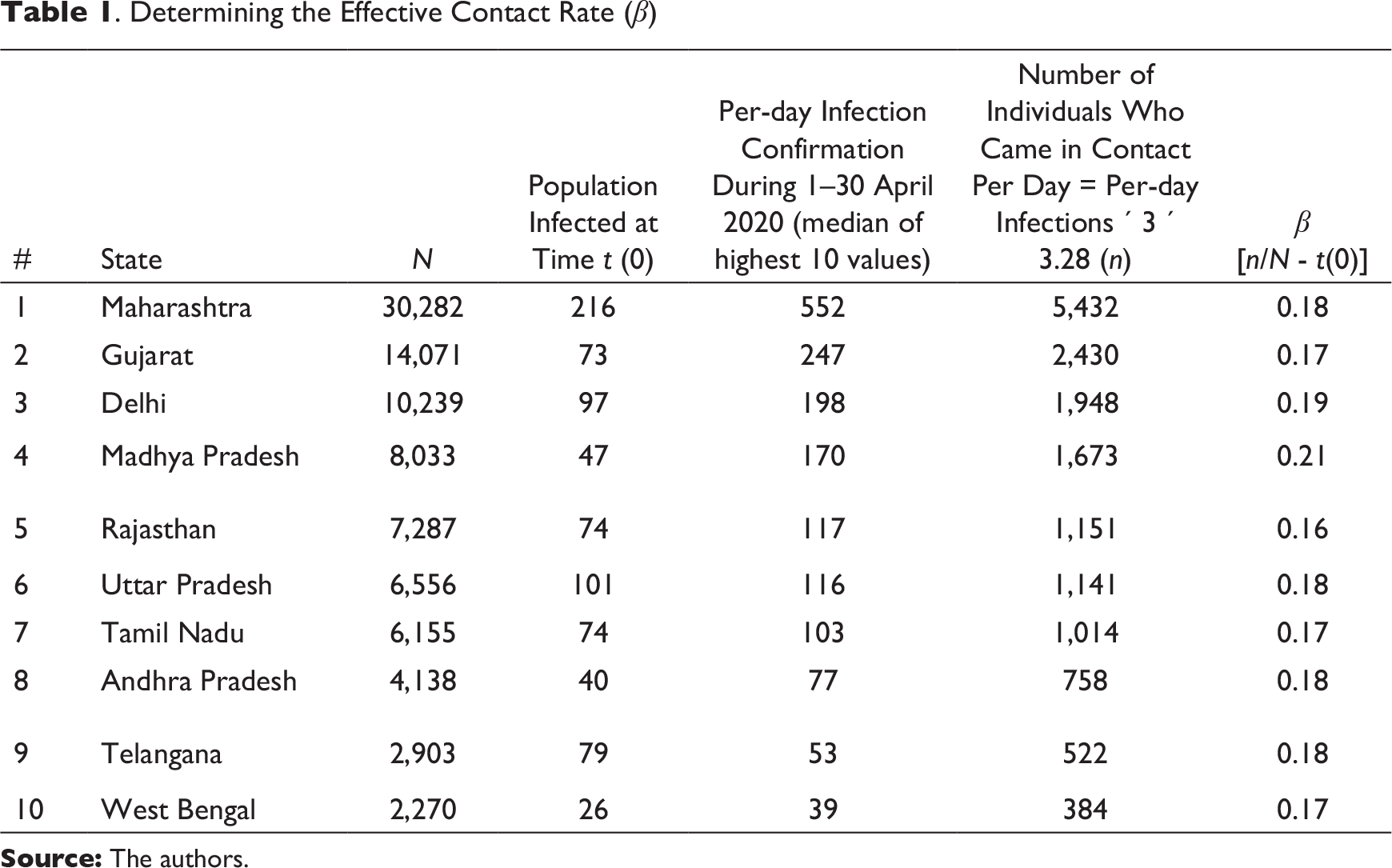
The effective contact rate (β)

The effective contact rate, β, is one of the two parameters of the SIR model that facilitate capturing the infection pattern in a population. It gives the proportion of susceptible population that an infected individual comes into contact with, per unit time (Hill, 2016).

βN = Total number of other individuals that infected individuals come into contact with per day, assuming the average infection time to be 3 days, that is, after 3 days the patient is confirmed as having COVID-19 (Batista, 2020):

Number of other individuals that an infected individual comes into contact with per day = per-day infections × 3 × 3.28

For example, let us say Delhi has an average daily infection of 300 individuals. On day (t) these 300 infected individuals are in contact with the susceptible population and thereby, infecting them. However, since it takes 3 days for an infected individual to be confirmed as a COVID-19 patient, the 300 infected individuals of day (t – 1) and day (t – 2) are also infecting the susceptible population on day (t). Therefore, on combining the previous two equations, the number of susceptible individuals who may have come in contact with the infected individuals is:

β N = Per-dayinfections \times 3 \times 3.28

Since β is the parameter of interest:

β = (Per-day infections \times 3 \times 3.28) / N

The values of per-day infections and N are different for each state. Hence, the values of parameter β are also different for each state.

Per-day infections (n)

The number of confirmed COVID-19 cases per day not only varies across states but also varies across the time period being considered (1–30 April 2020). Due to the fluctuating nature of the data, the following process was adopted to identify a representative figure for per-day infections. First, the 30 data points pertaining to confirmed cases during 1–30 April 2020 were sorted in an ascending order. Second, the median number of infections out of the ten highest values across the data was identified and considered as the number of infections per day. Due to the highly fluctuating nature of number of cases per day, the overall mean, median or quartile was not considered as an appropriate representative of per-day infections.

The removal rate (ύ)

The removal rate, ύ, is the inverse of the expected duration of infection (Jones, 2007). ύ is the second parameter of the SIR model that, along with β, facilitates capturing the infection pattern within a population. This is the post-infection duration during which the individual is removed from the population and, therefore, is not in a position to spread the infection. The expected duration of infection in the case of COVID-19 is around 30 days (Batista, 2020). Since ύ is the inverse of the expected duration of infection:

ύ = 1/Duration of infection = 1/30 = 0.03

The value of ύ is constant across states, since the duration of infection is likely to be independent of the state in which the infected person is treated.

Results

The values of the variables and effective contact rate parameter (β) for states are calculated as given in Table 1. The parameter values of N, t(0), β and ύ obtained from the data are run on Python 3.7.4 (Van Rossum & Drake, 2009) Jupyter Notebook (Kluyver et al., 2016) to model the expected lifecycle of COVID-19 in ten different states of India based on the SIR conceptual framework for the spread of viral diseases. The package Matplotlib 3.2.1 (Hunter, 2007) was used for deriving state-wise plots (Figure 1). The relevant Python codes to run the SIR model were borrowed from Hill (2016) and tweaked to suit the objectives of the present study.

Table 1

. Determining the Effective Contact Rate (β)

#	State	N	Population Infected at Time t (0)	Per-day Infection Confirmation During 1–30 April 2020 (median of highest 10 values)	Number of Individuals Who Came in Contact Per Day = Per-day Infections ´ 3 ´ 3.28 (n)	Β [n/N - t(0)]
1	Maharashtra	30,282	216	552	5,432	0.18
2	Gujarat	14,071	73	247	2,430	0.17
3	Delhi	10,239	97	198	1,948	0.19
4	Madhya Pradesh	8,033	47	170	1,673	0.21
5	Rajasthan	7,287	74	117	1,151	0.16
6	Uttar Pradesh	6,556	101	116	1,141	0.18
7	Tamil Nadu	6,155	74	103	1,014	0.17
8	Andhra Pradesh	4,138	40	77	758	0.18
9	Telangana	2,903	79	53	522	0.18
10	West Bengal	2,270	26	39	384	0.17

Source: The authors.

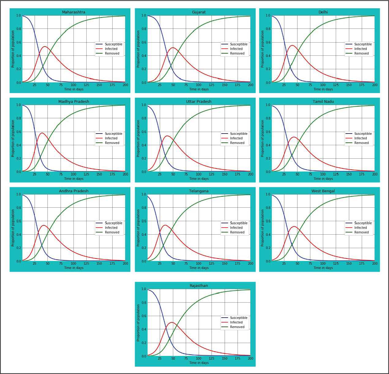
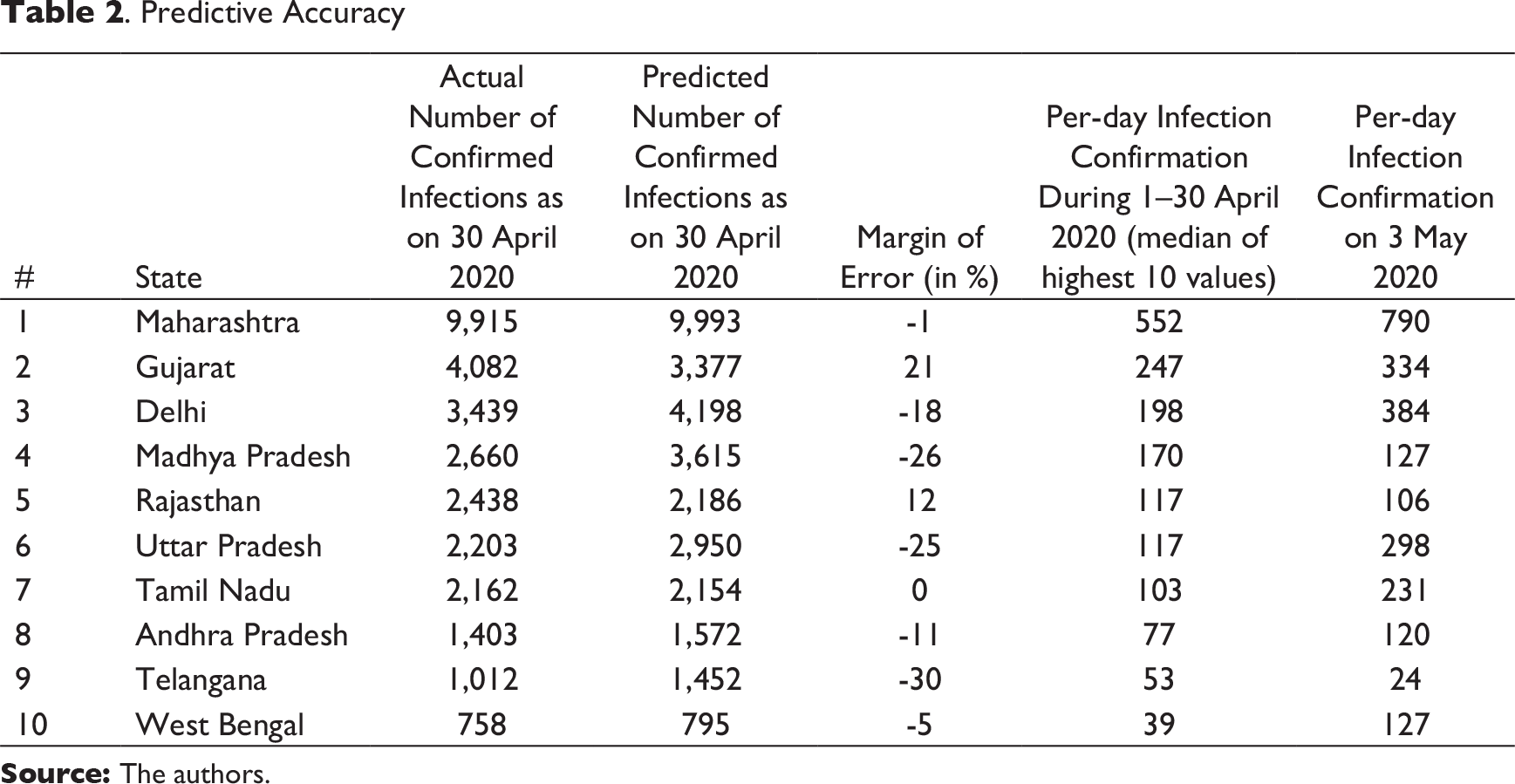
Using the package Matplotlib 3.2.1 (Hunter, 2007) and running the codes on Jupyter Notebook (Kluyver et al., 2016) IDLE, we obtained state-wise plots for ten states of India for determining information pertaining to: (a) the overall lifecycle and end date of the pandemic; (b) the peak date and the peak number of infected individuals; and (c) the predicted number of infected individuals as on 30 April 2020, so that the same could be compared vis-à-vis the actual data. The plots related to each of the ten states having the highest number of COVID-19-infected individuals as on 30 April 2020 is given in Figure 1. The predictive accuracy (Table 2), peak time and end time (Table 3) have been calculated based on the SIR plots given in Figure 1.

The output (Table 2) suggests the model has worked well for most of the states. Based on a comparative analysis between the actual data and predicted data as on 30 April 2020, the predictive accuracy of the model has been determined. The predictive accuracy is high for the states Maharashtra, Rajasthan, Tamil Nadu, Andhra Pradesh and West Bengal. This could be due to less variation in the number of confirmed cases per day. On the other hand, for Gujarat, Delhi, Madhya Pradesh, Uttar Pradesh and Telangana, the predictions have been moderately close to the actual figure. Again, the reason could be due to the following two factors. First, due to the variation in the number of confirmed cases per day, the calculated value of per-day infection confirmation during 1–30 April 2020 may not be a true representative of the per-day infections. A comparison of the representative value with per-day actual infection confirmation value as on 3 May 2020 (Table 2) reveals the discrepancy. This is due to the still-climbing rate of infections. Second, it is possible that the number of susceptible people each infected individual is infecting (R₀) could be less than the average value of 3.28, thereby affecting the total number of individuals who come in contact with COVID-19-infected individuals per day and, as a result, are getting infected (n).

Figure 1.

Source: The authors.

Table 2

. Predictive Accuracy

#	State	Actual Number of Confirmed Infections as on 30 April 2020	Predicted Number of Confirmed Infections as on 30 April 2020	Margin of Error (in %)	Per-day Infection Confirmation During 1–30 April 2020 (median of highest 10 values)	Per-day Infection Confirmation on 3 May 2020
1	Maharashtra	9,915	9,993	-1	552	790
2	Gujarat	4,082	3,377	21	247	334
3	Delhi	3,439	4,198	-18	198	384
4	Madhya Pradesh	2,660	3,615	-26	170	127
5	Rajasthan	2,438	2,186	12	117	106
6	Uttar Pradesh	2,203	2,950	-25	117	298
7	Tamil Nadu	2,162	2,154	0	103	231
8	Andhra Pradesh	1,403	1,572	-11	77	120
9	Telangana	1,012	1,452	-30	53	24
10	West Bengal	758	795	-5	39	127

Source: The authors.

Table 3.

Predicting the Peak Date and End Date

#	State	Peak Date	Predicted Number of Confirmed Infections as on Peak Date	End Date
1	Maharashtra	45 days: 15 May 20	16,352	180 days: 30 September 20
2	Gujarat	50 days: 20 May 20	7,317	185 days: 5 October 20
3	Delhi	40 days: 10 May 20	5,631	180 days: 30 September 20
4	Madhya Pradesh	40 days: 10 May 20	4,659	180 days: 30 September 20
5	Rajasthan	45 days: 15 May 20	3,644	180 days: 30 September 20
6	Uttar Pradesh	40 days: 10 May 20	3,606	180 days: 30 September 20
7	Tamil Nadu	45 days: 15 May 20	3,201	180 days: 30 September 20
8	Andhra Pradesh	42 days: 12 May 20	2,152	180 days: 30 September 20
9	Telangana	35 days: 5 May 20	1,597	175 days: 25 September 20
10	West Bengal	45 days: 15 May 20	1,180	180 days: 30 September 20

Source: The authors.

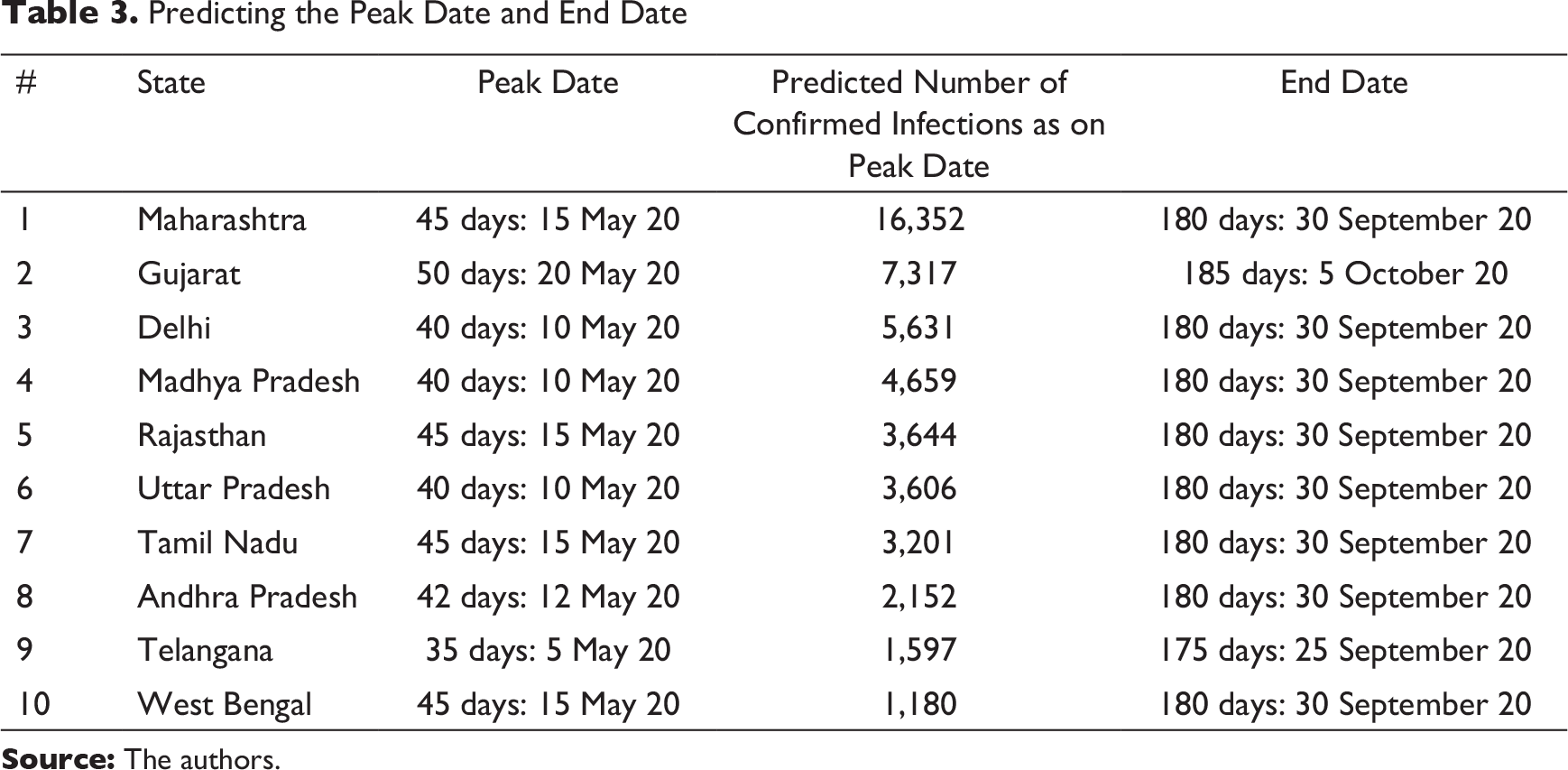
The output in Table 3 provides the likely number of days it would take for each state to reach the peak stage, as calculated from 1 April 2020 onwards. As per the present data, all the states are likely to reach the peak stage between 10 and 20 May 2020. The predicted number of cases as on the peak date has been calculated based on the proportion of infected individuals out of the total susceptible population as on the peak date. Further, based on culmination of the infection curve in each plot, the likely end date of the disease has been estimated for each state. All the states are likely to be under the influence of the disease for 175–185 days, as calculated from 1 April 2020. Thus, the influence of the COVID-19 pandemic in India is likely to last until the first week of October 2020.

Discussion and Conclusion

A model is only as good as the data available. Moreover, every model’s predictive accuracy depends on whether the assumptions are met. To what extent the available data reflects the true situation is questionable, because of limited testing during the early stages of the onset of the disease. This has resulted in the state-wise data having a lot of variations in terms of number of COVID-19-positive cases detected every day. Second, the study is based on the following major assumptions: (a) the total susceptible population of the state would be exposed to the virus for 3 months from the first date of data collection, that is, from 1 April 2020; (b) the median of the highest ten instances of confirmed cases per day during the month of April 2020 is representative of per-day infection confirmation; (c) an infected person continues to infect susceptible individuals in the population for 3 days until removed; and (d) each infected individual infects 3.28 other individuals per day. A violation in any of these assumptions results in a poor prediction. However, the findings of the study are in alignment with a similar international endeavour by Singapore University of Technology and Design’s (SUTD) Data-Driven Innovation Lab to predict the end date of the pandemic in various countries. This study by Luo (2020, May 5) predicts the theoretical end date of the pandemic in India to be in September 2020. Given the uncertainty and confusion surrounding the pandemic, our model is of some help to policymakers as well as ordinary citizens, giving them some form of timeline regarding the lifecycle of COVID-19 across ten states in India.

Footnotes

Declaration of Conflicting Interests

The authors declared no potential conflicts of interest with respect to the research, authorship and/or publication of this article.

Funding

The authors received no financial support for the research, authorship and/or publication of this article.

ORCID iD

Manit Mishra

References

Banik

Nag

Chowdhury

S. R.

Chatterjee

(2020). Why do COVID-19 fatality rates differ across countries? An explorative cross-country study based on select indicators. Global Business Review , 0972150920929897. http://doi/10.1177/0972150920929897.

Batista

(2020, May). FitVirusCOVID19 . https://in.mathworks.com/matlabcentral/fileexchange/74658-fitviruscovid19.

Bhattacharya

Paul

Biswas

(2015). Mathematical modeling of treatment SIR model with respect to variable contact rate. International Proceedings of Economics Development and Research , 83, 34–41.

Caccavo

(2020). Chinese and Italian COVID-19 outbreaks can be correctly described by a modified SIRD model. medRxiv . doi: https://doi.org/10.1101/2020.03.19.20039388.

Fernández-Villaverde

Jones

C. I.

(2020). Estimating and simulating a SIRD model of COVID-19 for many countries, states, and cities (No. w27128). National Bureau of Economic Research. https://www.nber.org/papers/w27128.

Hill

(2016). Learning scientific programming with Python . Cambridge University Press. Retrieved from https://scipython.com/book/.

Hunter

J. D.

(2007). Matplotlib: A 2D graphics environment. Computing in Science & Engineering , 9(3), 90–95.

Jones

J. H.

(2007). Notes on R _o . California: Department of Anthropological Sciences. https://web.stanford.edu/~jhj1/teachingdocs/Jones-on-R0.pdf.

Kermack

W. O.

McKendrick

A. G.

(1927). A contribution to the mathematical theory of epidemics. Proceedings of the Royal Society of London. Series A, Containing Papers of a Mathematical and Physical Character , 115(772), 700–721.

10.

Kluyver

Ragan-Kelley

Pérez

Granger

B. E.

Bussonnier

Frederic

Kelley

Hamrick

J.B.

Grout

Corlay

Ivanov

Avila

Abdalla

Willing

Jupyter Development Team (2016). Jupyter Notebooks—A publishing format for reproducible computational workflows (pp. 87–90). In Loizides

Scmidt

(Eds.), Positioning and power in academic publishing: Players, agents and agendas . IOS Press.

11.

M.Y.

Graef

J.R.

Wang

Karsai

(1999). Global dynamics of a SEIR model with varying total population size. Mathematical Biosciences , 160(2), 191–213.

12.

Liu

Gayle

A. A.

Wilder-Smith

Rocklöv

(2020). The reproductive number of COVID-19 is higher compared to SARS coronavirus. Journal of Travel Medicine . doi: 10.1093/jtm/taaa021.

13.

Luo

(2020). When will COVID-19 end? Data-driven prediction . https://ddi.sutd.edu.sg/.

14.

Muthuramakrishnan

Martin

(2016). SIR epidemic model with total population size. Advances in Applied Mathematical Biosciences , 7(1), 33–39.

15.

Rajkumar

(2020). COVID-19 in India: Dataset on Novel Corona virus disease 2019 in India . https://www.kaggle.com/sudalairajkumar/covid19-in-india.

16.

Van Rossum

Drake

F. L.

(2009). PYTHON 2.6 Reference Manual . PythonLabs.