Sage Journals: Discover world-class research

Abstract

Coronavirus disease 2019 (COVID-19) outbreak that was declared as a pandemic by the World Health Organization (WHO) on 11 March 2020 has already had severe consequences in all aspects of people’s lives worldwide. The pandemic has affected over 200 countries and has become a major concern. India also faced a stiff challenge in terms of controlling the virus outbreak and through some strict measures such as nationwide lockdown was able to control the further spread of COVID-19 towards the latter part of 2020. Therefore, it is imperative to predict the spread of this virus along with causality analysis of parameters that play a significant role in its spread. The present study employs a series of univariate and multivariate time series forecasting techniques namely MSARIMA, ARMAX and extended VAR models to predict COVID-19 cases in New Delhi, Mumbai and Bengaluru. Besides, providing a robust forecasting performance for COVID-19 cases, the study also deals with finding the causal relationship of the spread of COVID-19 with various mobility and weather parameters. Outcomes of our study establish that the spread of COVID-19 can be associated with mobility and weather parameters apart from the various precautions that are taken by the people to reduce community transmission. However, the type of mobility (residential, retail and workplace) and type of weather conditions (air quality, temperature and humidity) associated with the causality differ with cities. For New Delhi, air quality, residential, retail are the parameters affecting the spread of the COVID-19 cases, whereas masks, temperature, residential and workplace were the significant mobility and weather parameters for Mumbai. In addition, for Bengaluru, the statistically significant causal variables were air quality, masks and residential. Outcomes of this study would help the concerned authorities to predict and contain future COVID-19 spreads in Indian cities efficiently.

Keywords

COVID-19 India Time-Series Forecasting ARIMA ARMAX VAR Granger Causality

Introduction

Today, the world is facing an unprecedented outbreak of severe acute respiratory syndrome coronavirus 2 (SARS-CoV-2) or commonly referred to as coronavirus disease 2019 (COVID-19). On 11 March 2020, the World Health Organization (WHO) declared the COVID-19 outbreak as a pandemic and encouraged all countries to not only detect and test their people but also treat them by isolating the affected ones. Also, it advised the countries to contact trace the spread of the virus as it will help them prevent a handful of cases from becoming clusters and eventually leading to community transmission.

The virus that migrated from bats to humans first originated in Wuhan, China, rapidly spread to all Chinese provinces and since then has affected majorly all the countries of the world. China tried to contain the spread by undertaking some strict actions like suspension of activities such as public social gatherings or any mass activities, airport and highway closures along with railway interruptions. All these steps were aimed at minimizing the spread of community-level transmission, which is one of the leading factors for the high infection rate of the disease. Many other countries tried to control the initial spread by imposing nationwide lockdown but with time had to relax these rules in order to strike a fine balance between protecting the health of its people, minimizing economic and social disruption, and also respecting human rights. Though numerous efforts were put in place, the virus spread was not contained and till the time the WHO declared the novel coronavirus as a pandemic there were already 118,000 active cases in over 114 countries and 4,291 people had already lost their lives to this deadly virus. As of 2 February 2021, almost 102,942,987 cases have been reported worldwide with a total death count of 2,232,233. According to the WHO COVID-19 Dashboard, the worst affected countries are the USA, India, Brazil, France and Russia in terms of the total number of active cases. The virus that started by infecting a single individual later reached a scale where it is spreading at a cluster level and presently the situation is of community-level transmission making it all the more infectious.

India, with a population of 1.3 billion people, is not only the second-most populous country in the world but also has one of the highest population densities which makes India susceptible to large-scale community transmission, hence India was under the scanner of the whole world when the first confirmed cases of novel coronavirus were detected on 30 January 2020. It has been almost 10 months since the first confirmed case and India is the second worst affected country in the world in terms of the total number of active cases; however, in terms of deaths tally, the USA and Brazil fare much worse than India. In terms of total cases per million population as well as total deaths per million, India is doing better than the USA and other European Union countries which are experiencing second waves of COVID-19 with a potential risk of further new waves owing to ease in government restrictions (Dey, 2020).

In India, as the first few cases of COVID-19 infection surfaced, the government mandatorily started scanning not only the people travelling from China but also the people who had a recent travel history to China. Moreover, India was one of the few countries that imposed a nationwide lockdown when the number of confirmed cases was pretty low and still in a few hundred. The Indian Government announced the first nationwide lockdown on 23 March 2020 and it was for 21 days. Since the first lockdown, the government has kept on further extending the lockdown period to keep a check on the rising number of cases. Other important measures implemented by the government included contact tracing along with providing timely health care facilities to all those affected. Extensive testing was also carried out which was accomplished by setting up new facilities as well as converting some hotels and banquet halls into specialized COVID care units (‘Delhi hotels’, 2020). Although to strike a balance between protecting the health of its citizens and the economic health of the country, the government after three to four months of countrywide lockdown soon started gradually opening its economy basis red, orange and green zones created based on the active cases in that region. Various states have already started to recover from the different challenges that have helped them keep a check on the number of active cases. On the other hand, some states like Maharashtra, Delhi, etc. are still struggling to contain the number of rising cases.

Various research studies have been conducted worldwide to estimate the impact of coronavirus (Fardeen & Shareena, 2020; Sami, 2020 amongst others). Other studies (Abuhasel et al., 2020; Gurumurthy & Mukherjee, 2021; Nosier & Beram, 2020; Singh et al., 2020, among others) focused on forecasting the number of confirmed cases using various time series models to estimate the healthcare infrastructure requirements. Details of these studies have been provided in Table 1. As evident, the majority of these studies were with respect to China, the USA and other Asian and European Union countries and not much work has been done on India. The current study tried to bridge this gap.

Table 1.

Summary of Research Studies Focused on Forecasting COVID-19 Cases

Authors	Title	Country/Region	Model/Method	Major Outcomes
Singh et al. (2020)	Forecasting Daily Confirmed COVID-19 Cases in Malaysia Using ARIMA Models	Malaysia	ARIMA	The aim of this research is to first create a prediction model for regular reported COVID-19 cases using several covariates, and then to choose the best prediction model using a subset of these covariates
Katris (2020)	A Time Series-Based Statistical Approach for Outbreak Spread Forecasting: Application of COVID-19 in Greece	Greece	Epidemiological Model (tSIR)	The objective of this research is to develop a time series-based analytical data-driven methodology for tracking outbreaks
Abuhasel et al. (2020)	Analyzing and Forecasting COVID-19 Pandemic in the Kingdom of Saudi Arabia Using ARIMA and SIR Models	Saudi Arabia	Classical SIR Model, ARIMA	The well-known classical SIR model was used in the case of Saudi Arabia to estimate the highest number of cases that could be realized and the subsequent flattening of the curve. The ARIMA model, on the other hand, was used to estimate the prevalence of events
Nosier and Beram (2020)	Forecasting Covid-19 Infections and Deaths Horizon in Egypt (preprint)	Egypt	ARDL, ARIMA	The purpose of this study is to present a simple, parsimonious and accurate model for forecasting mortality caused by COVID-19. The presented Bass Model has compared it with several alternative existing models for forecasting the spread of COVID-19. Finally, some suggestions for limiting the virus’s spread and preventing new deaths as far as possible
Gurumurthy and Mukherjee (2021)	The Bass Model: A Parsimonious and Accurate Approach to Forecasting Mortality Caused by COVID-19	USA	Bass Model	The aim of this study is to present a clear, effective and accurate model for predicting COVID-19-related mortality. The presented Bass Model was compared to a number of other existing models for forecasting COVID-19 spread
Argawu (2020)	Modeling and Forecasting of COVID-19 New Cases in the Top 10 Infected African Countries Using Regression and Time Series Models (preprint)	Africa	Curve estimation regression, Time series models	Using data from 14 February to 6 September 2020, this analysis will model and forecast COVID-19 new cases in the top ten infected African countries (South Africa, Egypt, Morocco, Ethiopia, Nigeria, Algeria, Ghana, Kenya, Cameroon and Cote-dIvoire)
Iftikhar, H. and Iftikhar, M. (2020)	Forecasting Daily COVID-19 Confirmed, Deaths and Recovered Cases Using Univariate Time Series Models: A Case of Pakistan Study (preprint)	Pakistan	Univariate Time Series Models	They used AR, MA, ARMA, NPAR and SES models for forecasting confirmed, death and recovered cases for thorough policies shaping in this study
Zuhairoh and Rosadi (2020)	Real-Time Forecasting of the COVID-19 Epidemic Using the Richards Model in South Sulawesi, Indonesia	Indonesia	Richards Model	For the top five provinces in South Sulawesi, the goal is to create a model for the growth of COVID-19 cases and to predict when the pandemic will reach its peak of spread and when it will end
Sun et al. (2020)	Modeling and Forecasting the Spread Tendency of the COVID-19 in China	China	Improved SEIR Model	An improved SEIR model was developed to predict the spread of COVID-19 in China and to develop successful disease prevention strategies
Kola et al. (2020)	Forecasting COVID-19 Cases in Saudi Arabia Using Machine Learning SEIR and LSTM	Saudi Arabia	SEIR and LSTM	Using different machine learning models such as Sigmoid fitting, SEIR model and LSTM, the study aims to demonstrate in this article information-driven methods of forecasting the number of COVID-19 cases in Saudi Arabia 60 days ahead and the impacts of protective measures such as social isolations or COVID-19 lockout in the future
Jamshidi et al. (2020)	Modelling the Number of Confirmed Cases and Deaths from COVID-19 Pandemic in the UK and Forecasting over 15 April–30 May 2020	UK	Time Series Model	The current research focuses on the modelling and forecasting of the COVID-19 outbreak in the United Kingdom. This modelling was done using a two-part time series model to investigate the number of reported cases and deaths
Lakman (2020)	COVID-19 Mathematical Forecasting in the Russian Federation	Russia	ARIMA, SIRD and Holt–Winters exponential smoothing models	The paper provides an overview of current mathematical methods for forecasting COVID-19’s global trajectory. The newly established COVID-19 forecasting project office allowed the Russian Federation to identify the most successful analysis tools — the ARIMA, SIRD and Holt–Winters exponential smoothing models

Source: The author.

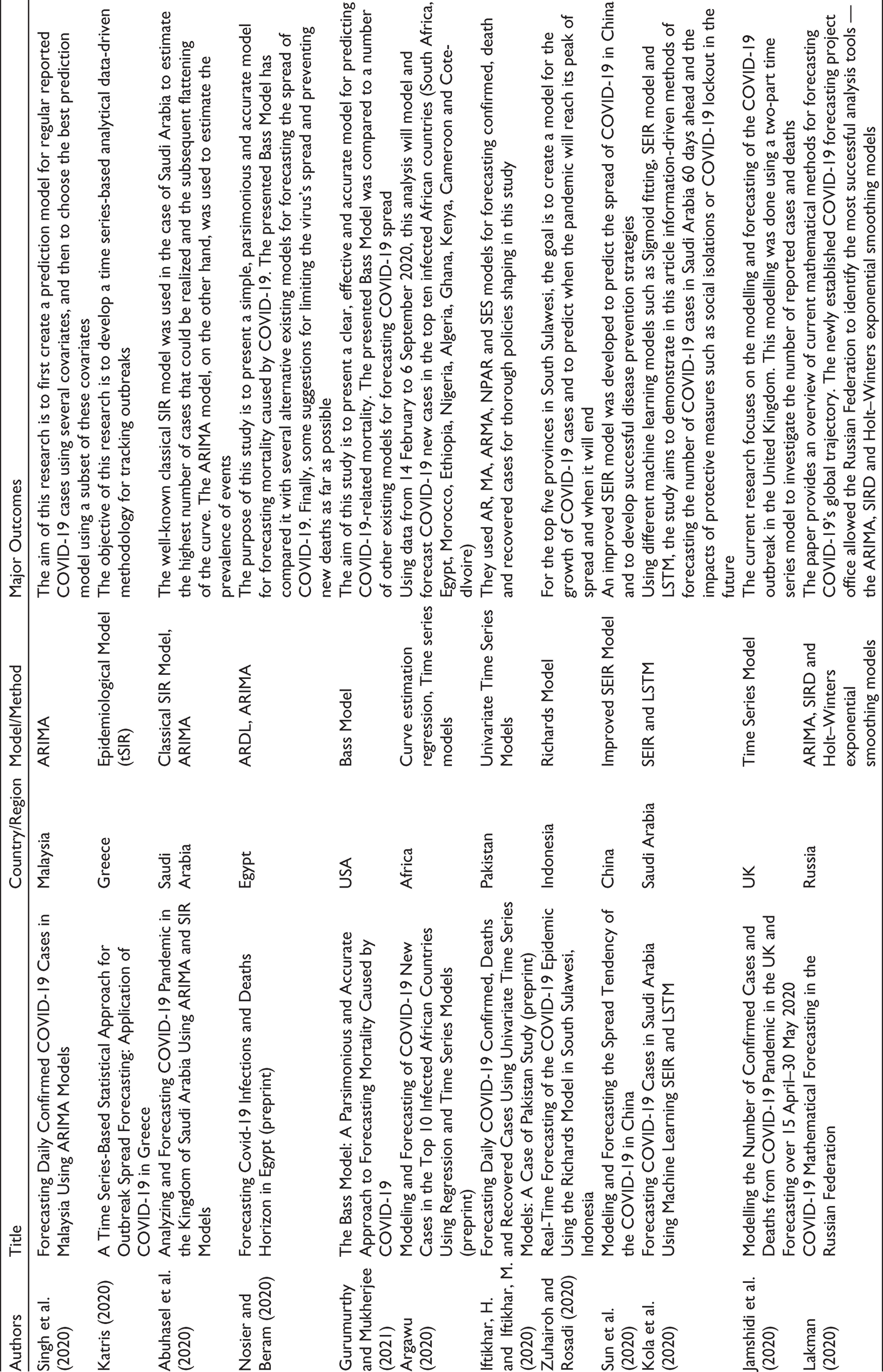
Gupta et al. (2020) presented a comprehensive analysis of the COVID-19 outbreak situation by answering different questions pertaining to the effects that various lockdown and social distancing measures had in curbing the number of coronavirus cases. Raju and Patil (2020) analysed the different Indian publications on SARS-CoV-2 and presented a bibliometric study of the WHO COVID-19 database whereas P. Ghosh et al. (2020) presented a state-wise analysis and prediction of the number of coronavirus cases. However, all these studies were conducted when the impact of coronavirus was limited to a few states that led to model performance being impacted by a limited number of data points. Also, no prior studies were conducted on the role played by mobility and weather parameters with respect to the spread of novel coronavirus.

We use a variety of univariate and multivariate models in this study to estimate and forecast the number of COVID-19 cases in three Indian cities: New Delhi, Mumbai and Bengaluru. In addition, the study also explores the connectedness between COVID-19 cases with different mobility and weather parameters.

All the models employed in this study provide forecasts with Mean absolute percentage error (MAPE) of less than 1%, thus providing a variety of accurate and robust methods for forecasting the number of cases in Indian cities. Also, our results point towards the relation that the spread of the novel coronavirus can be associated with mobility and weather parameters along with the precautions and other measures people are taking to reduce community transmission. However, the type of mobility (residential, retail and workplace) and type of weather conditions (air quality, temperature and humidity) associated with the causality differ across cities. The associated connectedness of COVID-19 cases with various mobility and weather-related factors can help in preventing the spread of the new strains that are emerging in different countries.

Materials and Methods

Data Sources and Description

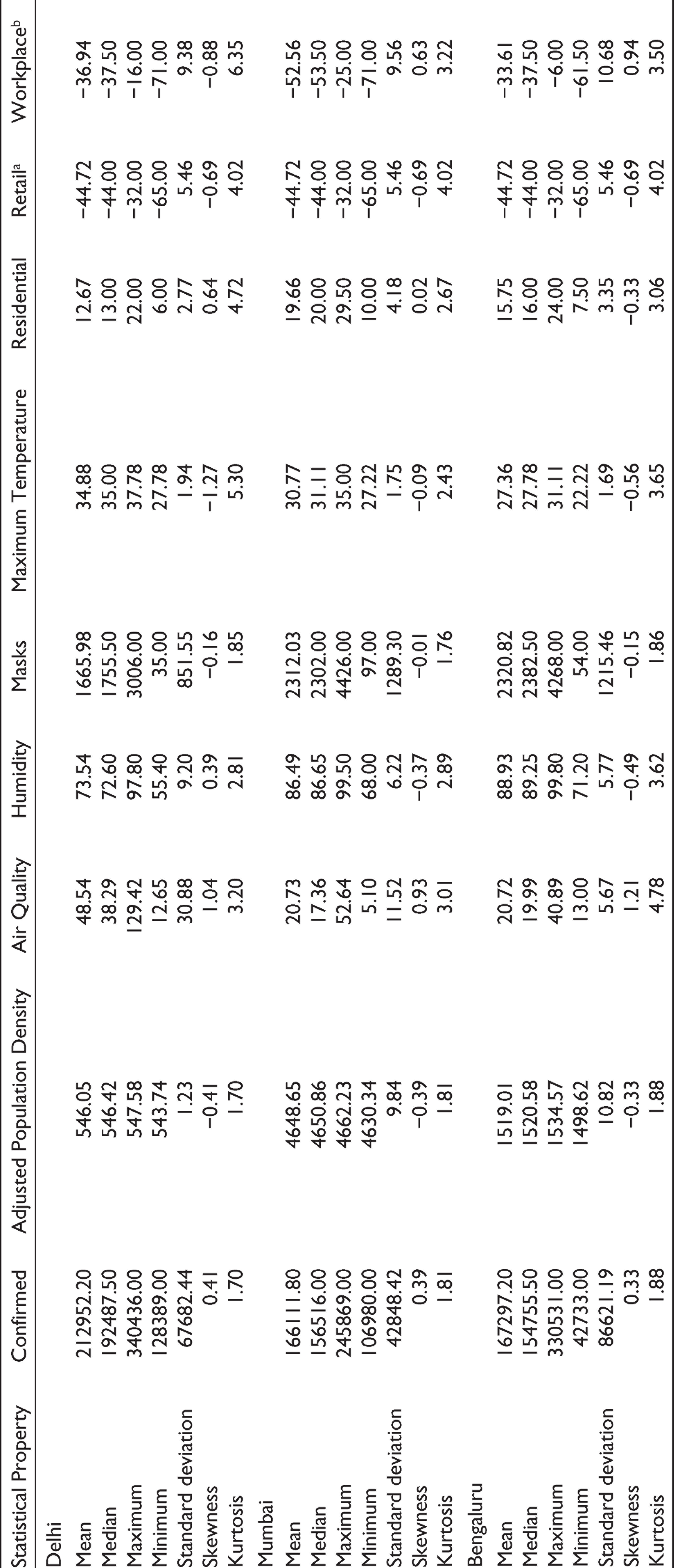
For the duration of 24 July 2020 to 21 October 2020, the data for confirmed COVID-19 cases in Delhi, Mumbai and Bengaluru were gathered from the website https://www.covid19india.org/. Data on the effect of the pandemic on mobility patterns in various locations were also collected for our study from Google’s Community Mobility Database. Google provides data for the Community Mobility Report, which tracks changes in mobility patterns for six different types of locations, which are

Retail and recreation—Visits to restaurants, cafes, shopping malls, amusement parks, museums, libraries, theatres and other similar establishments fall under this category

Grocery and pharmacy—Supermarkets, warehouses, farmers markets, specialty food stores and drug stores are included in this category

Parks—Beaches, marinas, dog parks, plazas and other public areas are included in this category

Transit stations—train stations including subways

Workplaces—office complexes

Residences—covers residential homes

It shows the change in mobility for every day of the week compared to the baseline (median during 3 January to 6 February 2020). But for this study, we have only considered mobility changes with respect to residential, workplaces and retail and recreation categories.

To take into account the weather parameters namely temperature and humidity, the data were collected from the website https://www.wunderground.com/. For assessing the impact of air quality (PM 2.5) on the number of COVID-19 cases in cities like New Delhi, Mumbai and Bengaluru, the data were collected from the website http://berkeleyearth.lbl.gov/air-quality/local/India

‘Adjusted population density’ is the immunity-adjusted population density. It is the population density multiplied by the square of the proportion of people who are still unprotected. It incorporates the effect of already affected individuals. Furthermore, ‘masks’ is the total amount of Google search interest observed by the different Indian states. It is a proxy indicator for people’s precautions and other efforts to minimize community transmission. People all over the world have begun to use masks, wash their mouths, refrain from touching their faces or shaking other people’s hands, disinfect public surfaces among other steps during this pandemic.

The rationale behind choosing these cities was that the lockdown measures must have had a significant impact on their mobility as they are amongst the biggest metropolitan cities in India along with having distinctive weather conditions.

Table 2 gives the summary statistics of the data for all the three cities under consideration.

Table 2.

Statistical Summary of the Data

Statistical Property	Confirmed	Adjusted Population Density	Air Quality	Humidity	Masks	Maximum Temperature	Residential	Retail^a	Workplace^b
Delhi
Mean	212952.20	546.05	48.54	73.54	1665.98	34.88	12.67	−44.72	−36.94
Median	192487.50	546.42	38.29	72.60	1755.50	35.00	13.00	−44.00	−37.50
Maximum	340436.00	547.58	129.42	97.80	3006.00	37.78	22.00	−32.00	−16.00
Minimum	128389.00	543.74	12.65	55.40	35.00	27.78	6.00	−65.00	−71.00
Standard deviation	67682.44	1.23	30.88	9.20	851.55	1.94	2.77	5.46	9.38
Skewness	0.41	−0.41	1.04	0.39	−0.16	−1.27	0.64	−0.69	−0.88
Kurtosis	1.70	1.70	3.20	2.81	1.85	5.30	4.72	4.02	6.35
Mumbai
Mean	166111.80	4648.65	20.73	86.49	2312.03	30.77	19.66	−44.72	−52.56
Median	156516.00	4650.86	17.36	86.65	2302.00	31.11	20.00	−44.00	−53.50
Maximum	245869.00	4662.23	52.64	99.50	4426.00	35.00	29.50	−32.00	−25.00
Minimum	106980.00	4630.34	5.10	68.00	97.00	27.22	10.00	−65.00	−71.00
Standard deviation	42848.42	9.84	11.52	6.22	1289.30	1.75	4.18	5.46	9.56
Skewness	0.39	−0.39	0.93	−0.37	−0.01	−0.09	0.02	−0.69	0.63
Kurtosis	1.81	1.81	3.01	2.89	1.76	2.43	2.67	4.02	3.22
Bengaluru
Mean	167297.20	1519.01	20.72	88.93	2320.82	27.36	15.75	−44.72	−33.61
Median	154755.50	1520.58	19.99	89.25	2382.50	27.78	16.00	−44.00	−37.50
Maximum	330531.00	1534.57	40.89	99.80	4268.00	31.11	24.00	−32.00	−6.00
Minimum	42733.00	1498.62	13.00	71.20	54.00	22.22	7.50	−65.00	−61.50
Standard deviation	86621.19	10.82	5.67	5.77	1215.46	1.69	3.35	5.46	10.68
Skewness	0.33	−0.33	1.21	−0.49	−0.15	−0.56	−0.33	−0.69	0.94
Kurtosis	1.88	1.88	4.78	3.62	1.86	3.65	3.06	4.02	3.50

Source: The author.

Notes: ^aNegative values showcase a dip to visits to retail and recreation areas, covering visits to restaurants, cafes, shopping centres, etc. as compared to the baseline period (median during 3 January to 6 February 2020). ^bNegative values showcase a dip to visits to workplace areas such as offices as compared to the baseline period (median during 3 January to 6 February 2020).

Models Description

In this study, three statistical models (ARMAX, SARIMA and VAR models) are used to predict the spread of COVID-19 in New Delhi, Mumbai and Bengaluru. Extended VAR model is used to understand the causal dynamics between the number of COVID-19 cases with weather and mobility parameters.

MSARIMA Model

A time series data set is essentially a data series that over time is collected consecutively. In any time series, an inherent feature of the data set is that the adjacent observations are naturally dependent. The study of this dependency is essentially considered as a sophisticated and commonly used model for forecasting and is referred to as time series analysis. Time series data usually include four components: secular trends, seasonal fluctuations, cyclical movements and random components. The movement of the business cycles that are captured by the cyclical aspect induces substantial changes over a long period. Therefore, for a short time period, it becomes extremely difficult to distinguish between secular trends and cyclical movements of the time series data set.

Msarima (x,y,z) (X,Y,Z)^s

MSARIMA belongs to the group of models known as univariate time series, which refers to a data set consisting of sequentially reported single observations over equal time intervals. Univariate analysis of a time series data set involves the usage of historical data from the variable in question to build a model that explains the behaviour of the variable. As a result, we can forecast using this constructed model. MSARIMA is an excellent technique to forecast a time series data set of high frequency where the effect of secular trends and seasonal fluctuations of a non-stationary time series Y_t is taken into account and expressed as:

Φ_{P} (B^{s}) φ_{P} (B) (1 B^{s}) {}^{D}{(1 B)} {}^{d}X_{t}^{} = Θ_{Q} (B {}^{s}) θ_{q} (B) u_{t}

(1)

where B is the backward shift operator, f and Φ are non-seasonal and seasonal autoregressive (AR) parameters while q and Θ are non-seasonal and seasonal moving average (MA) parameters, respectively. D is the order of seasonal differencing whereas d is the order of non-seasonal differencing.

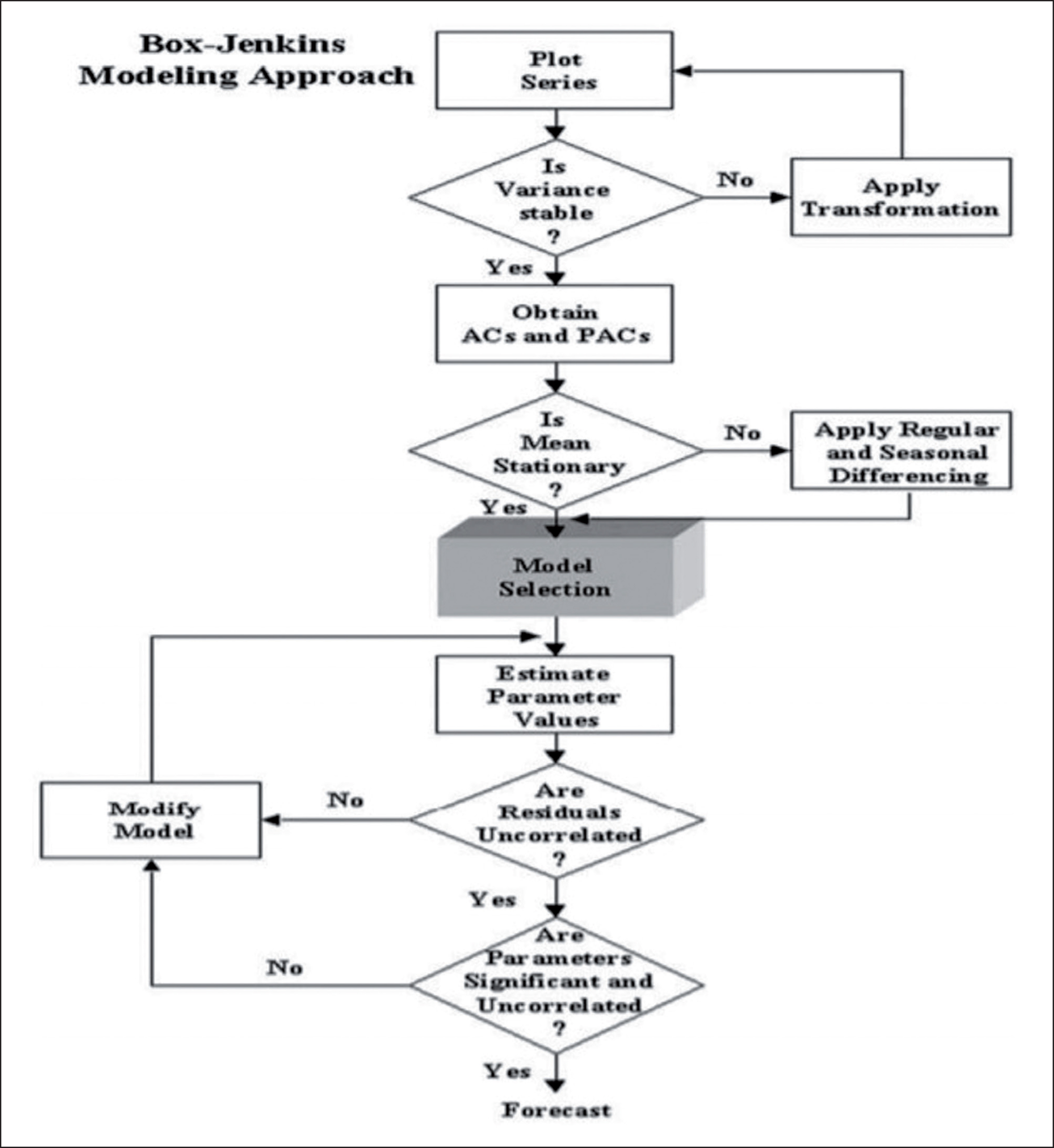
For any time series data set, it is essential to determine the MSARIMA model capable of generating the series. In other words, to make accurate predictions for the given time series which model should be considered that adequately captures its behaviour. This study employs the methodology developed by Box–Jenkins to identify the most appropriate model. It considers the model building as a reiterative process that can be divided into four stages: identification, estimation, diagnostic checking and forecasting which are explained below:

Identification: In this stage, appropriate AR and MA components are identified along with their seasonal counterparts based on the correlogram of the stationary form of the data series.

Estimation: Here, point estimates of the coefficients identified in earlier stage can be obtained by the method of maximum likelihood. Also, the provided associated standard errors along with t-statistics suggest the coefficients that can be dropped.

Diagnostic checking: This stage examines the residues of the estimated model to establish whether they have reached the white noise process.

Forecasting: Here, one tries to forecast the future values of the time series variable under-study after completion of the diagnostic checking process.

Flow chart of Box–Jenkins model building strategy is shown in Figure 1.

Figure 1.

Source: The author.

ARMAX Model

The ARMAX model is generally specified as:

X_{t} = Z_{t} ’ β + u_{t}

(2)

where Z_t’ is a (1 × h) vector containing h exogenous variables at time t, β is a (h × 1) vector of parameters and ut follows an ARMA(p, q)(P.Q) process.

The various exogenous variables used in this study are as follows:

Residential, Workplace, Retail that is the percentage changes in mobility with respect to the residential, workplace and retail and recreation categories from Google Mobility reports

Adjusted Population Density is the original population density times the square of the proportion of still vulnerable people. It incorporates the effect of already affected individuals.

Masks represent a proxy variable that measures the extent to which individual precautions are being taken by the people living in various states. For our study, ‘Masks’ is the cumulative Google search interest observed at state level. It serves as a proxy variable for precautionary measures people are taking to reduce community transmission.

Temperature represents the maximum temperatures in degree Celsius at state level.

Humidity represents state-level daily time series data on humidity.

Air quality represents state-level daily time series data on air quality measured using PM 2.5 levels.

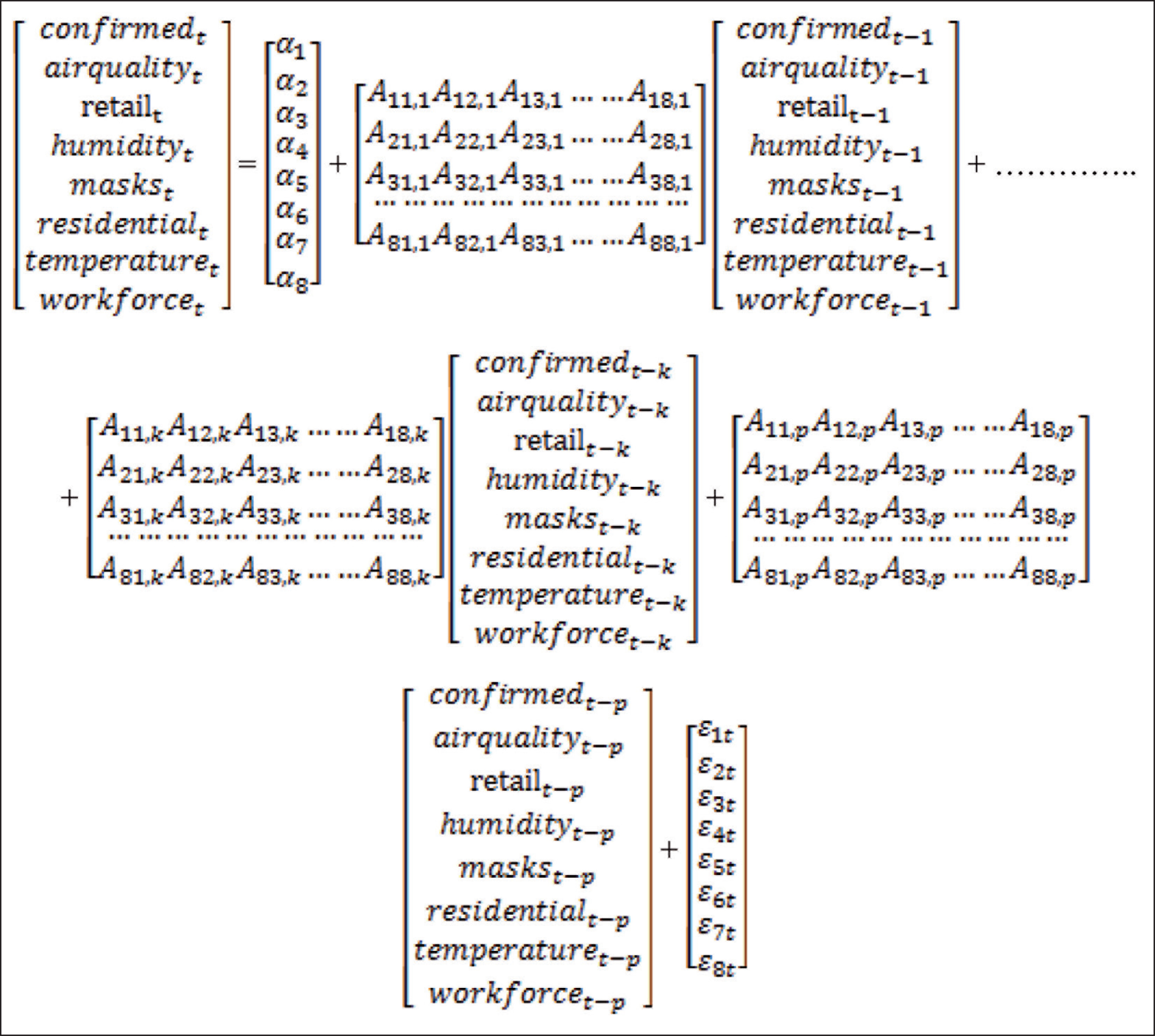
Toda Yamamoto Extended VAR Model

Traditional Granger causality tests are conditional on the presumption that the underlying variables are integrated of order zero in nature or stationary in an unrestricted VAR environment. The basic stability condition of the VAR is violated if the time series is non-stationary. This means that the tests used to determine the joint importance of the other lagged endogenous variables in VAR equations, such as the χ2 (Wald) test statistics for Granger causality, are no longer accurate. Co-integration must be investigated in the case of non-stationary data, and if it occurs, the vector error correction model should be used in place of unrestricted VAR. No long-term relationship test is used if the time series is not of order I(1) or is integrated with different orders. If tests like unit root and co-integration are used; however, they can have low power compared to the alternative. As a result, they could be misplaced and subject to pre-testing bias (Pesaran et al., 2001; Toda & Yamamoto, 1995).

To mitigate most of these problems, Toda and Yamamoto (1995) and Dolado and Lutkepohl (1996) limit the number of VAR(k) parameters using a modified Wald test, where k is the lag length of the VAR method. Using this method, the right order of the model (k) is increased by maximum integration order (d_max), then the VAR(k+d_max) is computed using the coefficients of the last lagged d_max vector. Toda and Yamamoto (1995) confirm that the Wald statistics converge with degrees of freedom equal to the number of the omitted lagged variables in distribution to a chi-square random variable, irrespective of whether the method is stationary, possibly around a linear pattern or co-integrated.

The Toda Yamamoto (TY) method is unique, firstly, since it does not necessitate pre-testing of the system’s co-integrating properties, which eliminates the potential for bias associated with unit roots and co-integration tests (Clarke & Mirza, 2006; Zapata & Rambaldi, 1997). Secondly, it suggests a causality test in a possibly arbitrary ordered system be it integrated or co-integrated using a higher VAR modelling standard, which allows for long-run details that are often ignored in systems that requires pre-whitening and first-differencing (Clarke & Mirza, 2006; Rambaldi & Doran, 2006) and finally the MWALD test statistics hold till the time the true lag length of the method is not exceeded by the process’s order of integration (Toda & Yamamoto, 1995).

However, there are some disadvantages to the TY method. Since the VAR model is purposefully over-fitted, the solution is ineffective and has some loss of power (Toda & Yamamoto, 1995, p. 247). For small sample sizes, Kuzozumi and Yamamoto (2000: 212) caution that the asymptotic distribution might be a poor approximation of the distribution of test statistics.

A VAR of order p can be represented by:

x_{t} = a_{0} + a_{1} t + \sum φ_{i} y_{t - 1} + ψ w_{t} + u_{t}

where x_t is a (m × 1) vector of endogenous variables, t is the linear time trend, a₀ and a₁ are (p × 1) vectors, w_t is a (q × 1) vector of exogenous variables and u_t is a (m × 1) vector of unobserved disturbances where u_t ~ N (0, Ω), t = 1, 2, …, T.

In our case, the TY version of the VAR(k+d_max) can be written as:

where d is the first-difference operator and (k + d_max) represents the order of p. By applying standard Wald tests to the first ‘k’ VAR coefficient matrix, we can detect the directions of Granger causality.

For example,

H₀₁: A_12,1 = A_12,2 = ……. = A_12,k = 0, suggests air quality does not Granger cause confirmed

H₀₂: A_21,1 = A_21,2 = ……. = A_21,k = 0, suggests confirmed does not Granger cause air quality

H₀₃: A_13,1 = A_13,2 = ……. = A_13,k = 0, suggests retail does not Granger cause confirmed

H₀₄: A_31,1 = A_31,2 = ……. = A_31,k = 0, suggests confirmed does not Granger cause retail and so on.

Model Performance Measures

Time series forecasting models can be assessed using the following commonly used accuracy measurement functions:

Root mean square error (RMSE) = $\sqrt{\frac{1}{N} \sum_{i = 1}^{N} (z_{i}} - {\bar{z}}_{i})$

Root mean square relative error (RMSRE) = $\sqrt{\frac{1}{N} \sum_{i = 1}^{N} } {(\frac{{\bar{z}}_{i} - z_{i}}{{\bar{z}}_{i}})}^{2}$

Mean absolute error (MAE) = $\frac{1}{N} \sum_{i = 1}^{N} | z_{i} - {\bar{z}}_{i} |$

MAPE = $\frac{1}{N} \sum_{i = 1}^{N} | \frac{z_{i} - z_{i}}{{\bar{z}}_{i}} |$

where z_I and ${\bar{z}}_{i}$ represent the actual and predicted values, respectively.

In this study, three statistical models (ARMAX, SARIMA and extended VAR models) are used for predicting the spread of the virus in three metropolitan cities in India, namely, New Delhi, Mumbai and Bengaluru along with causality analysis of weather and mobility parameters on the number of COVID-19 confirmed cases. The rationale behind choosing these cities was that the lockdown measures must have had a significant impact on their mobility as they are amongst the biggest metropolitan cities in India along with having distinctive weather conditions. To provide information regarding good model fit, each model’s performance was evaluated by using the above set of performance metrics.

Results and Discussion

For MSARIMA analysis, for each of the cities, either the de-trended series or de-seasonalized series or in some cases both were analysed as suggested by the correlogram of the original series. To make an MSARIMA(p,d,q)(P,D,Q)_s model, the AR order p and MA order q in a univariate ARMA model along with its seasonal components were identified using the autocorrelation function (ACF) and partial autocorrelation function (PACF) of the de-trended or de-seasonalized series or both. If then also, any autocorrelation remained, it was inspected in the residual series.

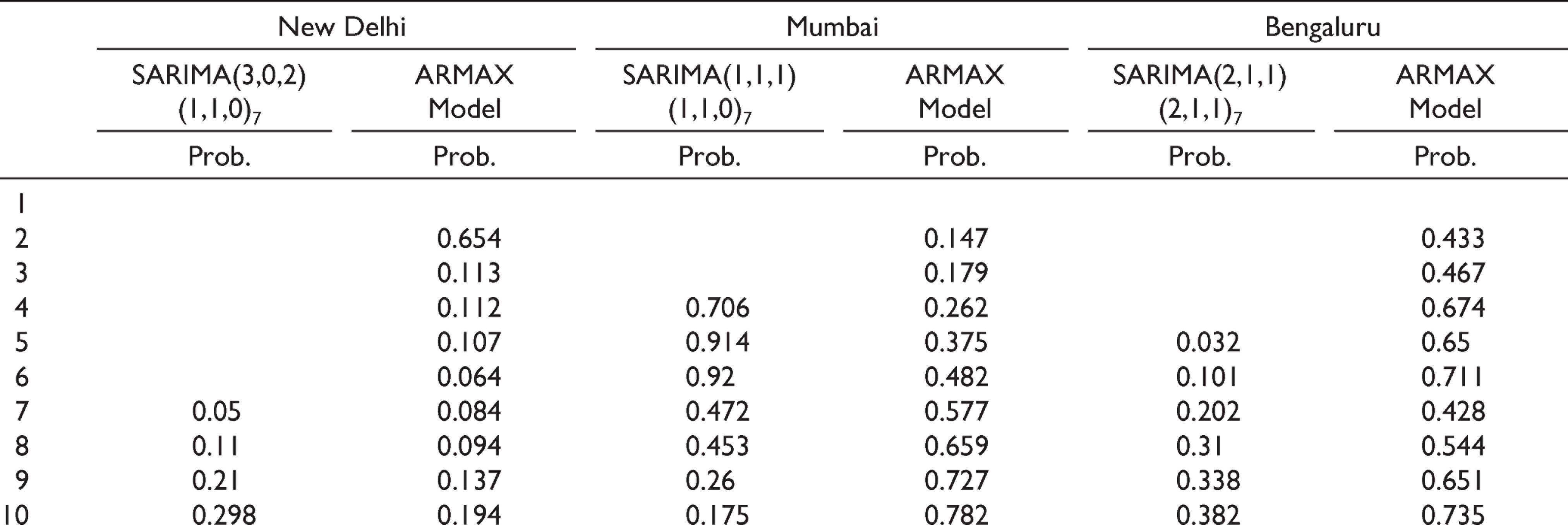
For New Delhi, we have found that SARIMA(3,0,2)(1,1,0)₇ model along with SARIMA(1,1,1)(1,1,0)₇ models for Mumbai and SARIMA(2,1,1)(2,1,1)₇ model for Bengaluru gives the best forecasting performance amongst various MSARIMA models. The estimated AR and MA parameters along with their seasonal components are found to be statistically significant at a 5% level. The stationarity as well as the invertibility conditions for respective seasonal and non-seasonal components, that is, AR and MA terms were also satisfied. Also, in all the cases, the residual series appears to be purely white noise as are shown in Table 4.

Table 3.

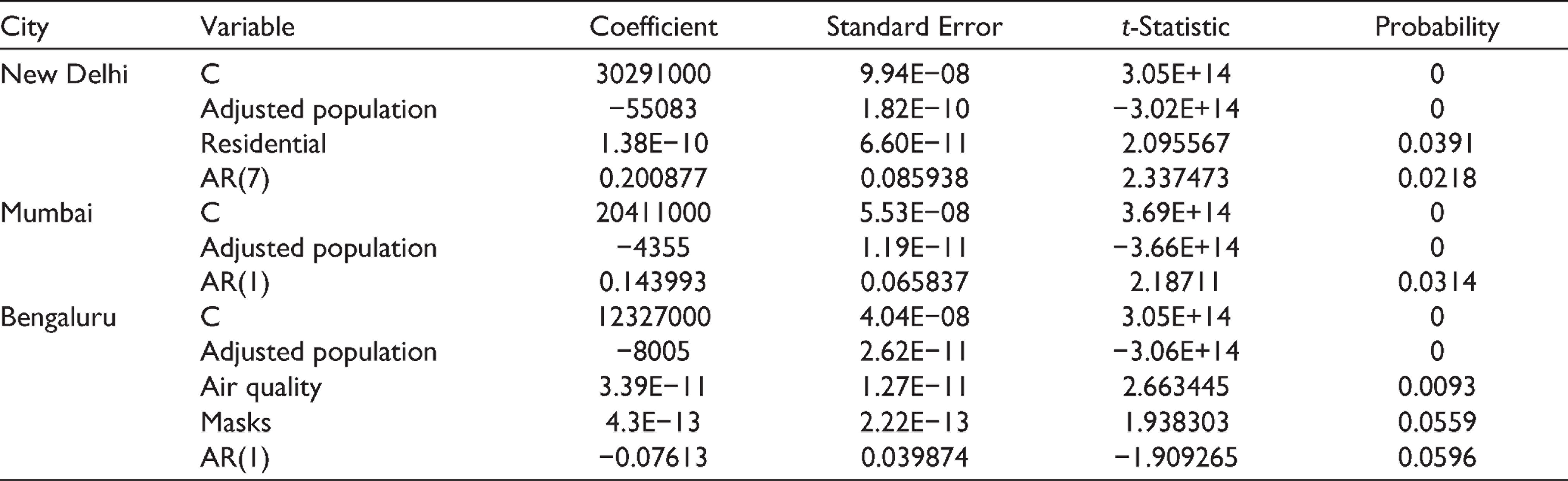
Estimated Parameters of ARMAX Model

City	Variable	Coefficient	Standard Error	t-Statistic	Probability
New Delhi	C	30291000	9.94E−08	3.05E+14	0
	Adjusted population	−55083	1.82E−10	−3.02E+14	0
	Residential	1.38E−10	6.60E−11	2.095567	0.0391
	AR(7)	0.200877	0.085938	2.337473	0.0218
Mumbai	C	20411000	5.53E−08	3.69E+14	0
	Adjusted population	−4355	1.19E−11	−3.66E+14	0
	AR(1)	0.143993	0.065837	2.18711	0.0314
Bengaluru	C	12327000	4.04E−08	3.05E+14	0
	Adjusted population	−8005	2.62E−11	−3.06E+14	0
	Air quality	3.39E−11	1.27E−11	2.663445	0.0093
	Masks	4.3E−13	2.22E−13	1.938303	0.0559
	AR(1)	−0.07613	0.039874	−1.909265	0.0596

Source: The author.

Table 4.

Probability Values for Residual Series Depicting White Noise for Different Models

	New Delhi		Mumbai		Bengaluru
	SARIMA(3,0,2)(1,1,0)₇	ARMAX Model	SARIMA(1,1,1)(1,1,0)₇	ARMAX Model	SARIMA(2,1,1)(2,1,1)₇	ARMAX Model
	Prob.	Prob.	Prob.	Prob.	Prob.	Prob.
1
2		0.654		0.147		0.433
3		0.113		0.179		0.467
4		0.112	0.706	0.262		0.674
5		0.107	0.914	0.375	0.032	0.65
6		0.064	0.92	0.482	0.101	0.711
7	0.05	0.084	0.472	0.577	0.202	0.428
8	0.11	0.094	0.453	0.659	0.31	0.544
9	0.21	0.137	0.26	0.727	0.338	0.651
10	0.298	0.194	0.175	0.782	0.382	0.735
11	0.344	0.262	0.186	0.826	0.488	0.796
12	0.459	0.205	0.257	0.861	0.053	0.827
13	0.576	0.243	0.332	0.889	0.083	0.877
14	0.642	0.147	0.098	0.911	0.11	0.674
15	0.72	0.189	0.089	0.928	0.144	0.719
16	0.694	0.206	0.112	0.941	0.109	0.763
17	0.724	0.089	0.15	0.952	0.134	0.814
18	0.793	0.115	0.196	0.948	0.079	0.653
19	0.78	0.13	0.238	0.947	0.097	0.653
20	0.792	0.045	0.244	0.494	0.114	0.711
21	0.844	0.05	0.294	0.537	0.059	0.765
22	0.879	0.049	0.341	0.551	0.057	0.811
23	0.836	0.048	0.393	0.507	0.032	0.849
24	0.864	0.064	0.447	0.52	0.043	0.793
25	0.89	0.082	0.316	0.565	0.055	0.781
26	0.892	0.091	0.37	0.614	0.071	0.801
27	0.692	0.107	0.414	0.659	0.087	0.84
28	0.663	0.121	0.412	0.7	0.1	0.848
29	0.718	0.092	0.449	0.738	0.125	0.879
30	0.731	0.11	0.413	0.773	0.072	0.903
31	0.692	0.129	0.432	0.803	0.086	0.901
32	0.741	0.155	0.483	0.831	0.09	0.907
33	0.785	0.094	0.521	0.854	0.073	0.898
34	0.77	0.108	0.563	0.875	0.085	0.92
35	0.808	0.129	0.508	0.893	0.096	0.884
36	0.764	0.155	0.392	0.909	0.112	0.879

Source: The author.

Results of the estimated ARMAX models are shown in Table 3. Adjusted population density appears to be the only statistically significant exogenous variable for all the cities which influence the number of COVID-19 confirmed cases. Apart from adjusted population density, the percentage change in residential mobility for New Delhi along with masks and air quality parameters for Bengaluru were other statistically significant exogenous variables. In addition, for New Delhi there are statistically significant seasonal ARMA(1,0) components, for Mumbai and Bengaluru there are statistically significant non-seasonal ARMA(1,0) components. The residual series, as shown in Table 4, appears to be white noise.

In the next stage, we estimate the VAR model. For New Delhi, the order of the VAR based on the AIC (Akaike information criterion) and HQ (Hannan-Quinn information criterion) is found to be 7. Similarly, for Mumbai and Bengaluru the order of the VAR was found out to be 2 and 7, respectively.

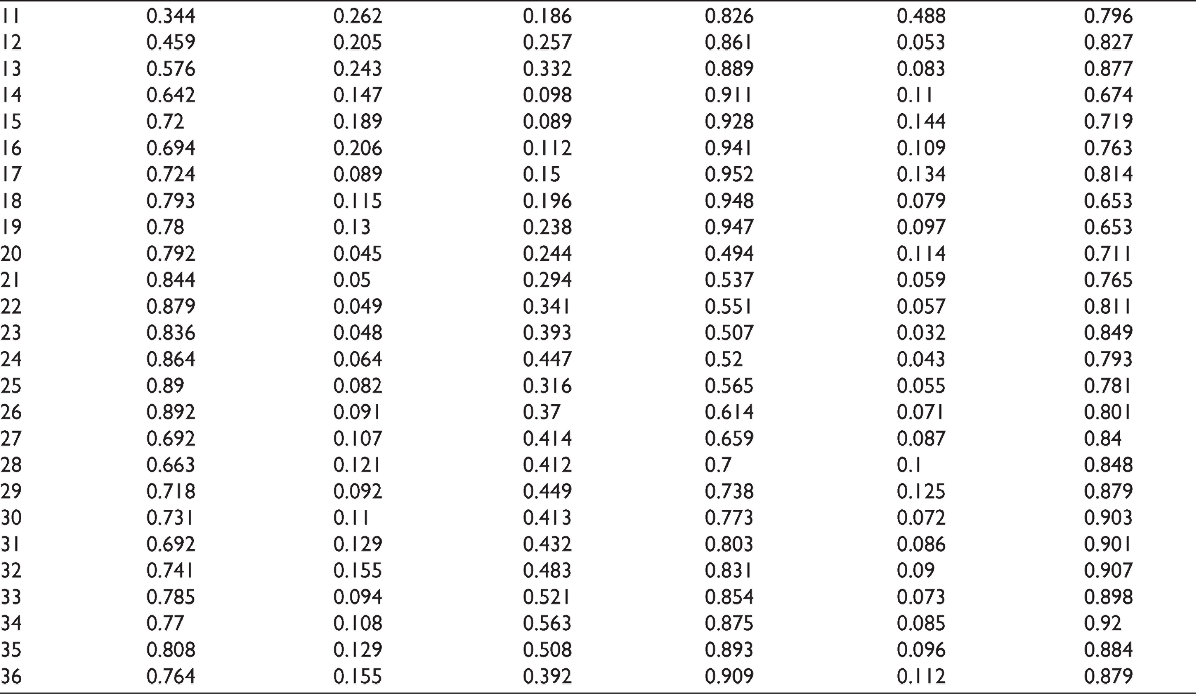
Estimated ARMAX, MSARIMA and VAR models are finally used to forecast COVID-19 confirmed cases for the period 21 September 2020 to 21 October 2020, and the forecasts are then evaluated based on MAE, RMSE and MAPE, which are standard performance criterion used in time series forecasting. Two performance criteria, that is, RMSE and MAE usually depend on the scale of the variable. On the other hand, MAPE is generally not sensitive to the variable’s scale. The forecasting performance of the series is better if the errors are smaller.

As shown in Table 5, MAPE values between actual and predicted values by the three models, that is, MSARIMA, ARMAX and extended VAR models for the last one month (21 September to 21 October) of the data span is less than 1. Also, it is evident that the ARMAX model slightly outperforms the other two models.

Table 5.

Forecasting Performance

City	Model	RMSE	MAE	MAPE
New Delhi	MSARIMA Model SARIMA(3,0,2)(1,1,0)₇	185.8043	129.7836	0.04095
	ARMAX Model	2.42E-09	2.06E-09	6.95E-13
	Extended VAR Model	96.90699	82.82325	0.028537
Mumbai	MSARIMA Model: SARIMA(1,1,1)(1,1,0)₇	370.0051	334.8674	0.1434
	ARMAX Model	6.76E-10	1.37E-10	5.62E-14
	Extended VAR Model	392.2006	312.1433	0.143511
Bengaluru	MSARIMA Model: SARIMA(2,1,1)(2,1,1)₇	482.4084	392.9664	0.1299
	ARMAX Model	6.62E-10	5.95E-10	2.12E-13
	Extended VAR Model	106.0432	80.37353	0.031043

Source: The author.

Results of Granger causality after running the extended VAR model are shown in Table 6.

Table 6.

Granger Causality Tests (Linear)

Null Hypothesis of Non-Causality; χ² (2) Statistics
New Delhi (VAR 8)^a
	Confirmed	Air Quality	Retail	Humidity	Masks	Residential	Temperature	Workforce
Confirmed		9.96154(0.2677)	4.712719(0.7878)	14.44906(0.0708)	9.774819(0.2812)	6.211198(0.6236)	40.98912(0.000)	7.225592(0.5125)
Air quality	14.19061(0.0769)	Not the focus area
Retail	20.0459(0.0102)
Humidity	8.689458(0.3692)
Masks	3.887522(0.8671)
Residential	21.39409(0.0062)
Temperature	4.144472(0.08439)
Workforce	3.246236(0.918)
Mumbai (VAR 3)^a
Confirmed		3.028990(0.0818)	0.015031(0.9024)	0.256206(0.6127)	0.486304(0.4856)	3.447119(0.0634)	0.186653(0.6657)	1.206210(0.2721)
Air quality	2.643027(0.104)	Not the focus area
Retail	2.426966(0.1193)
Humidity	0.868853(0.3513)
Masks	38.2629(0.0000)
Residential	11.75219(0.0006)
Temperature	4.718427(0.0.298)
Workforce	7.071621(0.0078)
Bengaluru (VAR 8)^a
Confirmed		7.461902(0.5891)	8.166725(0.5174)	27.38664(0.0012)	14.45272(0.1071)	11.14329(0.2660)	2.685870(0.9755)	19.84737(0.0189)
Air quality	19.32122(0.0226)	Not the focus area
Retail	7.883101(0.546)
Humidity	14.64555(0.1011)
Masks	25.41936(0.0025)
Residential	15.59492(0.0758)
Temperature	9.540158(0.389)
Workforce	10.709(0.2962)

Source: The author.

Note: ^aIn extended VAR, order of VAR is inflated by the maximum order of integration which in our case is 1.

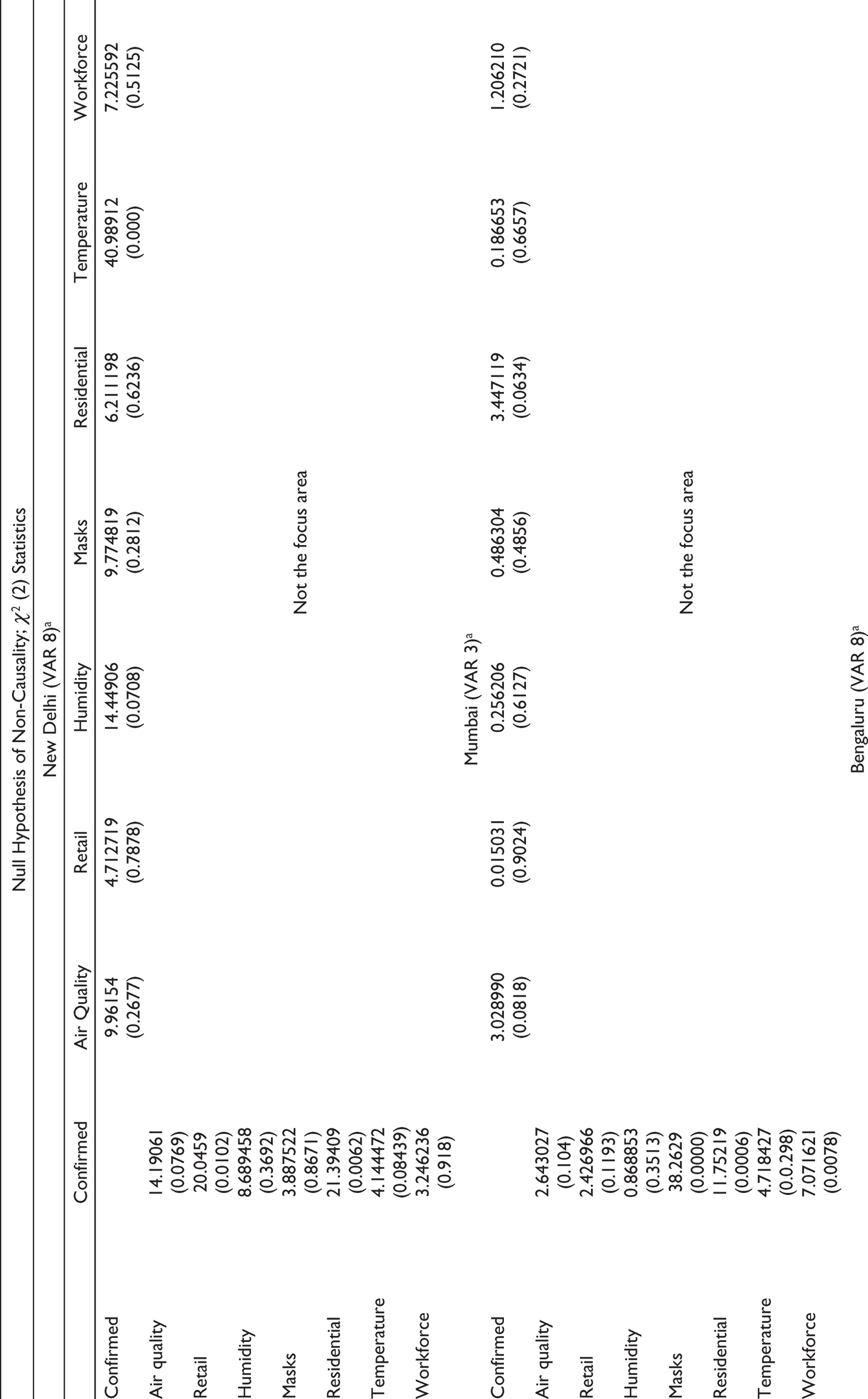
For New Delhi, air quality, residential and retail variables were statistically significant at a 10% confidence interval. Hence, the Granger causality runs from all these statistically significant variables to the number of COVID-19 confirmed cases. Similarly, for Mumbai, masks, temperature, residential and workplace were the statistically significant variables, suggesting that the Granger causality runs from all these statistically significant variables to COVID-19 confirmed cases.

For Bengaluru, the statistically significant variables were air quality, masks and residential, suggesting that the Granger causality runs from all these variables to COVID-19 confirmed cases.

Conclusion

In this study, univariate and multivariate time series techniques are used for forecasting COVID-19 cases in three Indian cities namely New Delhi, Mumbai and Bengaluru. All the models explored have lower forecasting errors; however, it was found that ARMAX slightly outperforms other models. One of the contributions of this study is that it develops robust forecasting models to predict COVID-19 cases. The models explored in this study provide very low forecasting errors (MAPE of less than 1%), thus providing a variety of accurate and robust methods for forecasting the number of cases. It also helps in finding the causal relationship of the spread of COVID-19 with various mobility and weather parameters. In addition, the study also establishes the connectedness between COVID-19 cases with various mobility and weather-related factors.

It was found that ARMAX models outperform both MSARIMA and extended VAR in terms of forecasting daily confirmed cases in the three studied cities. For New Delhi, ARMAX models suggest that the increase in COVID-19 confirmed cases is only influenced by adjusted population density and percentage change in residential mobility. Similarly, the ARMAX model suggests that masks and air quality parameters for Bengaluru were the other statistically significant exogenous variables. The statistical significance of residential, masks and air quality exogenous variables in some cities points towards the relation that the spread of the novel coronavirus can be associated with mobility and weather parameters along with the precautions and other measures people are taking to reduce community transmission. This argument is further strengthened by the results of the Granger causality tests, which states that certain mobility parameters along with weather conditions influence the spread of COVID-19. However, the type of mobility (residential, retail and workplace) and type of weather conditions (air quality, temperature and humidity) associated with the causality differ with cities.

For New Delhi and Bengaluru, as air quality is one of the causal variables, it points to the fact that exposure to air pollution may increase the risk of contracting the COVID-19 infection. Hence, the concerned authorities should especially pay attention to the poor communities, who are at greater risk of contracting the COVID-19 infection, as they are more susceptible to be exposed to indoor air pollution. For preventing the further spread of the COVID-19 virus, monitoring air quality should also be counted as an important aspect of public health protection. For Mumbai, as masks represent one of the causal variables, it points to the fact that the concerned authorities should further strive towards raising awareness about the precautions and other measures they should be taking to reduce community transmission. Wearing masks, disinfecting public surfaces, not touching their faces or shaking other people’s hands, washing hands, etc. are some of the steps that should be constantly advertised.

The availability of a novel coronavirus vaccine is a positive step towards the eradication of this pandemic; however, the emergence of new COVID-19 strains has raised serious concerns about the efficacy of the newly developed vaccine. The associated connectedness of COVID-19 cases with various mobility and weather-related factors can help in preventing the spread of the new strains.

Footnotes

Declaration of Conflicting Interests

The author declared no potential conflicts of interest with respect to the research, authorship and/or publication of this article.

Funding

The author received no financial support for the research, authorship and/or publication of this article.

References

Abuhasel

K. A.

, Khadr

, & Alquraish

M. M.

(2020). Analyzing and forecasting COVID-19 pandemic in the Kingdom of Saudi Arabia using ARIMA and SIR models. Computational Intelligence, 1–14

Argawu

A. S.

(2020). Modeling and forecasting of COVID-19 new cases in the top 10 infected African countries using regression and time series models. MedRxiv. https://doi.org/10.1101/2020.09.23.20200113

Clarke

, & Mirza

S. A.

(2006). Comparison of some common methods of detecting Granger noncausality. Journal of Statistical Computation and Simulation, 76, 207–231.

COVID19India.com (2020). India COVID-19 tracker: City wise confirmed cases. https://www.covid19india.org/

Delhi hotels step up the game, turn into COVID Care Centres (2020, 30 June. Times of India. https://timesofindia.indiatimes.com/travel/travel-news/delhi-hotels-step-up-the-game-turn-into-covid-care-centres/as76703125.cms

Dey

(2020). COVID-19: Second waves emerge in many countries. Is India ready? DownToEarth. https://www.downtoearth.org.in/blog/health/covid-19-second-waves-emerge-in-many-countries-is-india-ready--70872

Dolado

J. J.

, & Lütkepohl

(1996). Making Wald tests work for cointegrated VAR systems. Econometric Review, 15, 369–386.

Fardeen

, & Shareena

(2020). An empirical study on impact of covid-19 on the businesses. https://papers.ssrn.com/sol3/papers.cfm?abstract_id=3700339

Ghosh

, Ghosh

, & Chakraborty

(2020). COVID-19 in India: State-wise analysis and prediction. Medrxiv. https://doi.org/10.1101/2020.04.24.20077792

10.

Gola

, Arya

, Animesh

, Dugh

, & Khan

(2020). Fine-tuned forecasting techniques for COVID-19 prediction in India. MedRxiv. https://doi.org/10.1101/2020.08.10.20167247

11.

Griebe

(2020). COVID-19 mobility model. https://www.stat-vision.com/2020/05/29/covid-19-mobility-model/

12.

Gupta

, Pal

, & Pandey

(2020). A comprehensive analysis of COVID-19 outbreak situation in India. Medrxiv. https://doi.org/10.1101/2020.04.08.20058347

13.

Gurumurthy

, & Mukherjee

(2021). The Bass Model: a parsimonious and accurate approach to forecasting mortality caused by COVID-19. International Journal of Pharmaceutical and Healthcare Marketing, 14(3). https://www.emerald.com/insight/content/doi/10.1108/IJPHM-06-2020-0056/full/html

14.

Iftikhar

, & Iftikhar

(2020). Forecasting daily COVID-19 confirmed, deaths and recovered cases using univariate time series models: A case of Pakistan study. MedRxiv. https://doi.org/10.1101/2020.09.20.20198150

15.

Jamshidi

, Rezaei

, Kakavandi

, & Jamshidi Zargaran

(2020). Modeling the number of confirmed cases and deaths from the COVID-19 pandemic in the UK and forecasting from April 15 to May 30, 2020. Disaster Medicine and Public Health Preparedness, 1–7.

16.

Katris

(2020). A time series based statistical approach for outbreak spread forecasting: Application of COVID-19 in Greece. Expert Systems with Applications, 166, 114077. https://www.sciencedirect.com/science/article/abs/pii/S0957417420308368?via%3Dihub

17.

Kola

, Veena

, & Guntoju

(2020). Forecasting COVID-19 cases in Saudi Arabia using machine learning SEIR and LSTM. Journal of Green Engineering, 10(5).

18.

Kuzozumi

, & Yamamoto

. (2000). Modified lag augmented autoregressions. Econometric Review, 19, 207–231.

19.

Lakman

I.A.

, Agapitov

A.A.

, Sadikova

L.F.

, Chernenko

O.V.

, Novikov

S.V.

, Popov

D.V.

, Pavlov

V.N.

, Gareeva

D.F.

, Idrisov

B T.

, Bilyalov

A.R.

, & Zagidullin

N.Sh.

(2020). Possibilities of mathematical forecasting of coronavirus infection in the Russian Federation. Arterial Hypertension, 26(3), 288–294

20.

Nature.com (2020). Coronavirus latest: pandemic could have killed 40 million without any action. https://www.nature.com/articles/d41586-020-00154-w

21.

Nosier

, & Beram

(2020). Forecasting Covid-19 infections and deaths horizon in Egypt. MedRxiv. https://www.medrxiv.org/node/98707.external-links.html

22.

Pesaran

M. H.

, Smith

R. J.

, & Shin

(2001). Bounds testing approaches to the analysis of level relationships. Journal of Applied Econometrics, 16(3), 289–326.

23.

Raju

, & Patil

(2020). Indian publications on SARS-CoV-2: a bibliometric study of WHO COVID-19 database. Medrxiv. https://doi.org/10.1101/2020.06.08.20125518

24.

Rambaldi

A. N.

, & Doran

T. E.

(2006). Testing for Granger non-causality in cointegrated system made easy [Working Papers in Econometrics and Applied Statistics No. 88]. Department of Econometrics, University of New England.

25.

Sami

(2020). Impact of covid-19 pandemic on global economy. https://papers.ssrn.com/sol3/papers.cfm?abstract_id=3700302

26.

Singh

, Murali Sundram

, Rajendran

, Boon Law

, Aris

, Ibrahim

, Chandra Dass

, & Singh Gill

(2020). Forecasting daily confirmed COVID-19 cases in Malaysia using ARIMA models. The Journal of Infection in Developing Countries, 14(9), 971–976.

27.

Singhal

(2020). A review of coronavirus disease-2019 (COVID-19). The Indian Journal of Pediatrics, 87(4), 281–286.

28.

Sun

, Duan

, Xiong

, & Wang

(2020). Modeling and forecasting the spread tendency of the COVID-19 in China. Advances in Difference Equations, (1), 1–16.

29.

Toda

H. Y.

, & Yamamoto

(1995). Statistical inference in vector auto-regressions with partially integrated processes. Journal of Econometrics, 66, 225–250.

30.

Zapata

H.O.

, & Rambaldi

A.N.

(1997). Monto Carlo evidence on cointegration and causation. Oxford Bulletin of Economics Statistics, 59, 285–298.

31.

Zuhairoh

, & Rosadi

(2020). Real-time forecasting of the COVID-19 epidemic using the Richards Model in South Sulawesi, Indonesia. Indonesian Journal of Science and Technology, 5(3), 456–462.

Forecasting COVID-19 Confirmed Cases in Major Indian Cities and Their Connectedness with Mobility and Weather-related Parameters

Abstract

Keywords

Introduction

Materials and Methods

Data Sources and Description

Models Description

MSARIMA Model

Msarima (x,y,z) (X,Y,Z)s

ARMAX Model

Toda Yamamoto Extended VAR Model

Model Performance Measures

Results and Discussion

Conclusion

Footnotes

Declaration of Conflicting Interests

Funding

References

Msarima (x,y,z) (X,Y,Z)^s