Sage Journals: Discover world-class research

Abstract

Historical trends are widely analysed in financial market research for their long-term influence on stock indices. The current research examines the impact of historical volatility on NIFTY 50 returns on the basis of daily data from 2009 to 2025. The research aims to highlight the impact of historical volatility on market performance. The study employs a five-step econometric modelling for building an ARDL model for NIFTY returns by using historical volatility as an independent variable. We have performed ARDL and ARDL bound tests for finding short- and long-term relationship between the variables, respectively. The results of the study reveal a short- and long-term significant relationship between historical volatility and NIFTY returns. The ARDL bound test and diagnostic check validate the model’s robustness and long-term predictive value. The study’s results have implications for market participants, policymakers and researchers in understanding return predictability and market efficiency in the Indian stock market.

Keywords

Historical volatility ARDL model econometric modelling NIFTY 50 volatility–return dynamics

Introduction

NIFTY 50 is a major benchmark index that represents the Indian stock market. Several factors influence the performance of NIFTY, including macroeconomic indicators, investors’ sentiments as well as historical trends (Hingane et al., 2023; Megaravalli & Sampagnaro, 2018). The study of historical trends is important to understand the market pattern, market trends and time series investment behaviour. The historical data are used to determine the recurring cycles, assess the efficiency of the market and develop predictive models for future trends and forecasting (Kumar et al., 2021; Toromade & Chiekezie, 2024). Thus, it is crucial to understand the interrelation between historical market trends.

While making investment decisions, it is crucial to understand the relationship between historical market trends and NIFTY returns. Though past performance does not always guarantee future returns, it does enable investors, researchers and investigators to inquire about factors that drive market movements, which include identifying the pattern and assessing the risk (Malkiel, 2003). The current research will look at how historical data can be used to better understand market behaviour, determine the effect of volatility and refine investment strategies. The current study will determine whether past time trends are in sync with the NIFTY returns. The existing literature on the current topic has extensively examined the various aspects in relation to NIFTY returns and volatility, including the impact of volatility during specific events (e.g., demonetization), modelling and forecasting volatility using different statistical techniques, and understanding the divergence between historical and implied volatility. Prior research studies have not sufficiently addressed both the short- and long-run dynamics using different time frames and events. The study aims to bridge the gap by providing an analysis of historical returns. The main objective of the current research is to find out the impact of historical volatility on NIFTY return by using daily data. The research aims to contribute to the field of financial market analysis and investment decision-making by using historical market data. The research will provide valuable takeaways for investors and traders in navigating market fluctuations and long-term investment strategies. The research is grounded in an extensive literature review and utilizes secondary data for the years 2009–2025. The period from 2009 to 2025 captures a broad spectrum of market conditions, including post-global financial crisis, multiple policy reforms (such as GST and demonetization), the COVID-19 pandemic impact and the recent economic stabilization and growth. The insights from the study will not only enrich our comprehension of the Indian stock market but also help in shaping policies to instil financial stability and investors’ confidence in the Indian equity market.

Origin of Financial Market and Importance of Historical Data

The origin of the stock market may be traced back to the early practice of trading between merchants and bankers in Europe (Poitras, 2012). Since its beginning, the stock market has grown into a complex system that arranges for the creation of capital and opportunities for investment and economic growth (Gomes & Gubareva, 2021).

The Indian stock market is regulated by the Securities and Exchange Board of India (SEBI). It is a very important part of the Indian financial system (Kaur, 2018; Sabarinathan, 2010). Analysing historical data is essential for understanding trends assessing risk and making informed investment decisions. It provides insights into past market fluctuations, economic cycles and investor behaviour. This information allows the market analysts to identify patterns that may influence future performance. The investors use investor historical data to evaluate market corrections, bulls and beer phases and the impact of macroeconomic events on stock returns.

Understanding NIFTY Returns

NIFTY 50 is one of the premier stock indices of India, a weighted benchmark of 50 large-cap stocks listed at the National Stock Exchange (NSE). The index reflects the market sentiment and stability of the economy, where returns from NIFTY are nothing but the appreciation or depreciation of the value of listed indices within the period due to factors such as the corporate earnings of the companies and macroeconomic conditions. The trends of the global market, along with the investor decision-making process, are significantly influenced by various economic, political, and technological factors (Sahu, 2015; Subburayan, 2017). Intraday, weekly, monthly and yearly measurements of stock returns are common; hence, based on the trends in historical return series, the investor tries to focus on future movements of the market. The factors behind the fluctuation in the return of NIFTY include inflation, interest rate, financial institution investors’ (FIIs) inflow and outflow, and geopolitical situation. The comprehension of these variations is important for the investor to optimize the investment strategies with a minimum level of risk.

Literature Review

Theoretical Background and Divergent Views on Volatility and Returns

The relationship between past volatility and stock market movement has been extensively studied and has produced mixed results depending on market conditions and the economy (Schwert, 1989). The efficient market hypothesis (EMH) states that financial markets are efficient in themselves, and past performance or prices have no influence on the future expected returns (Ali et al., 2021; Malkiel, 1989, 2003; Shiller, 2003). According to EMH, using past values to forecast NIFTY returns would be ineffective, especially in efficient markets. Conversely, several research studies have observed that historical volatility does influence future returns, particularly in emerging markets, where inefficiencies are more common. On the other hand, several studies conducted on emerging economies and some that have been conducted in the Indian context confirmed that past winners continue to outperform past losers (Beloskar & Nageswara Rao, 2024; Locke & Gupta, 2009; Pandey & Sehgal, 2016). Technical indicators such as moving averages and relative strength indices (RSI) do provide signals for NIFTY returns (Dongrey, 2022; Waghela et al., 2024). This view suggests that markets are not entirely efficient and that investor psychology and sentiment, influenced by past volatility, play a significant role in decision-making. The strong relationship between past performance and returns has been related to inefficiency (Rosenberg et al., 1998). Such results may indicate that past volatility influences investors’ expectations and trading decisions and, therefore, can lead to return predictability.

Several research studies have conducted studies to observe the impact of historical market trends on future returns (Chandra, 2012; Durham et al., 2005; Mukherjee & Roy, 2016; Snowden, 1990). Two contradictory views have emerged in the literature: some studies have established that historical data have an impact on returns (Awan et al., 2021; Goetzmann et al., 2001; Kahn & Rudd, 1995; Merton, 1980), whereas other studies have shown that there is no significant relationship between them (Banz, 1981; Huy et al., 2021; Merton, 1980).

Empirical Studies Supporting the Predictive Power of Historical Volatility

Several studies support the argument that historical volatility impacts future stock returns. The studies confirm that volatility is a measure of market risk that reflects uncertainty in price movements (Mishra et al., 2025). Studies have shown that historical volatility significantly impacts future returns; the higher volatility in the past is often associated with increased market risk and fluctuating return patterns (Engle, 2004; Lundblad, 2007; Muguto & Muzindutsi, 2022; Schwert, 1989). The research has confirmed that the historical periods of high volatility are generally followed by a long string of price fluctuations (Poon & Granger, 2003; Xiuzhen et al., 2022). The research has reflected a strong correlation between past levels of VIX and subsequent NIFTY returns (Chakrabarti & Kumar, 2020; Mukherjee & Mandal, 2024) such that historical volatility seems to determine the risk perception and investors’ decisions (Huber et al., 2022; Klos et al., 2005). This reinforces the argument that past volatility serves as an indicator of market sentiment and potential return shifts (Chu et al., 2022; Lee et al., 2002). Historical spiking of volatilities, including that at the time of financial crisis, found that such instances suppress returns in the near future as investors behave more cautiously in subsequent times (Bouri & Harb, 2022; Yang, 2024).

Empirical Studies Challenging the Predictive Role of Historical Volatility

While many studies demonstrate a connection between historical volatility and returns, others argue against any significant relationship. Some findings support the EMH by showing that historical data lack predictive power, with no consistent influence on future market movements (Banz, 1981; Huy et al., 2021; Merton, 1980). These studies highlight that any apparent patterns may be spurious or arise from over-fitting in certain models. The findings established that historical analysis is inefficient or has no predictive power and thus would be ineffective in predicting NIFTY movements.

Empirical Approaches for Analysing and Modelling of Historical Volatility and NIFTY Returns

A study, using the GARCH model, revealed that historical volatility exhibits the clustering effect, meaning that periods of high volatility tend to be followed by continued turbulence. To study the impact of historical volatility on NIFTY returns, several modelling techniques have been used in the past, ranging from traditional statistical models to advanced machine learning systems (Kashyap, 2023). Earlier studies relied on Autoregressive Integrated Moving Average (ARIMA)–based models, where they used past patterns to examine the underlying pattern. This demonstrated that short-term price trends captured by ARIMA-based forecasting models were successful, but they failed to account for sudden shock (Borges et al., 2024; Ospina et al., 2023; Raza et al., 2024). There are other better models like Generalized Auto-regressive Conditional Heteroscedasticity (GARCH) that have been widely employed to measure persistent volatility (Chang & Tsai, 2008; Yurttagüler, 2024).

Machine learning methods have also been explored for the volatility–return relationship further (Kashyap, 2023; Zhong & Enke, 2019). Long short-term memory (LSTM) networks have been utilized for analysing historical NIFTY data and also for forecasting. It was found that deep-learning models significantly outperformed traditional methods in modelling relationships between volatility and return. They have been proven to bring improved return prediction based on historical market behaviour (Alkhatib et al., 2022; Shah et al., 2022). The recent rise in the role of AI-driven market forecasting for real-time prediction based on historical data is established in research (Chakraborty & Parida, 2024; Pillai, 2023).

Though there is extensive research work on historical volatility and market returns, there exist several gaps within the literature. Most of these studies focus on daily or short-term volatility measures, opening the question about how weekly, monthly or yearly historical volatility impacts NIFTY returns (Mishra et al., 2025). The research has been conducted on technical analysis but in isolation without using different time frames and events. GARCH and ARIMA have been widely used, but their predictive power is limited during extreme market events (Borges et al., 2024; Shah et al., 2019). The potential of advanced machine learning models analysing long-term volatility trends remains unexploded, especially in the context of Indian markets. The study bridges this gap as it explores historical volatility’s effect on NIFTY returns using daily data for a very long period, which covers different time frames and events.

From the scope of the objective of the present research, aimed at determining the historical volatility-affected NIFTY returns using daily data points, hypotheses are built for the current research. Previous studies suggested that shorter market movements are highly sensitive to volatility due to speculative trading and rapid sentiment shift (Baker & Wurgler, 2007; Ben Osman et al., 2024; Poon & Granger, 2003). If confirmed, this hypothesis indicates that investors react strongly to recent fluctuations when making weekly investment decisions.

H₁: Historical volatility has a significant impact on daily NIFTY returns.

Research Methodology

Data

The daily data of NIFTY returns from January 2009 to January 2025 (15 years) have been captured from the official website of the NSE of India. The data then have been utilized to calculated historical volatility of daily NIFTY return data.

First, we calculate historical volatility from the daily data of NIFTY returns. Then, we compute the log returns as follows:

r_{t} = I n (P_{t} / P_{t}_{- 1})

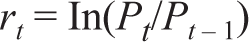
Where

r_t = Daily log return on day t

P_t₌ Closing price on day t

P_t_–1 = Closing price on day t–1

To calculate historical volatility, first, we compute the standard deviation of the returns using the following formula:

σ = \sqrt{\frac{1}{N - 1}} \sum_{t =!}^{N} {(R_{t} - \bar{R})}^{2}

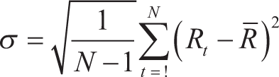
Where

σ = Historical volatility

(R_t – R–)² = log return at time t

R– = Average log return over the period

N = Number of observations (days)

We have taken standard deviation of the log return to capture historical volatility.

The Econometric Research Methods

In the first step, we perform unit root testing for the NIFTY returns and the historical volatility for daily data. To assess the stationarity of data, we use augmented Dickey–Fuller (ADF) test and Kwiatkowski–Phillips–Schmidt–Shin (KPSS) test of the time series under study. Upon checking the unit root, we found that the series are integrated at different levels. The series of independent variable is integrated at I(1), which indicates that the series is first difference stationary, while that of the dependent variable is integrated at I(0), indicating level stationary. Then, we run the Bai–Perron test for structural break (Bai & Perron, 2003). We have identified five potential breakpoints in the data. The optimal number of breakpoints is determined by the point at which the Bayesian information criterion (BIC) reaches its minimum.

In the second step, we proceed with model identification when the series are integrated at I(1) and I(0) combination we use ARDL to test the relationship between the variables (Nkoro & Uko, 2016). To test short-term relationship between variables, we have used ARDL regression models, while to test long-term relationship between the variables, we have used ARDL bound test (Sarkodie & Owusu, 2020).

Then, the third step is model specification. To apply the ARDL model, we first select suitable lags of dependent and independent variables. For optimum lag selection, we have used the Akaike Information Criterion (AIC).

As the next step after performing the ARDL bound test, we have done diagnostic testing of the regression models. For the diagnostic test, we have used the serial correlation test (Breusch–Godfrey LM test), heteroscedasticity test (Breusch–Pagan test or white test), normality test (Jarque–Bera Test) and model stability check (CUSUM and CUSUMSQ tests).

We have used R-studio to perform the statistical method on the time series.

Data Analysis and Interpretation

Step 1: Unit Root Test

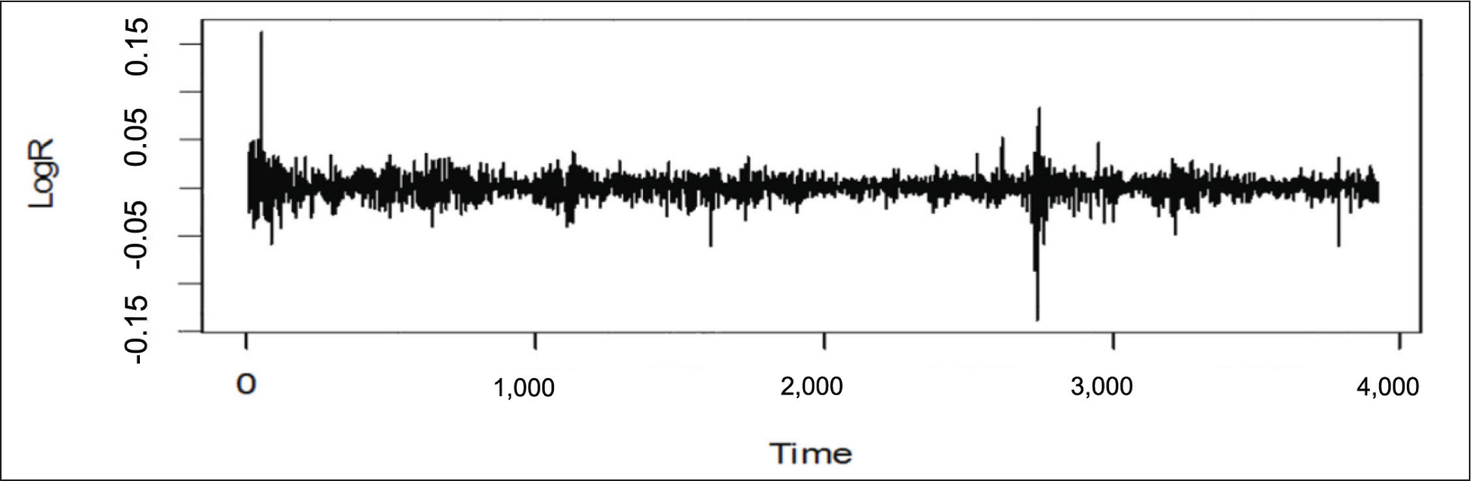
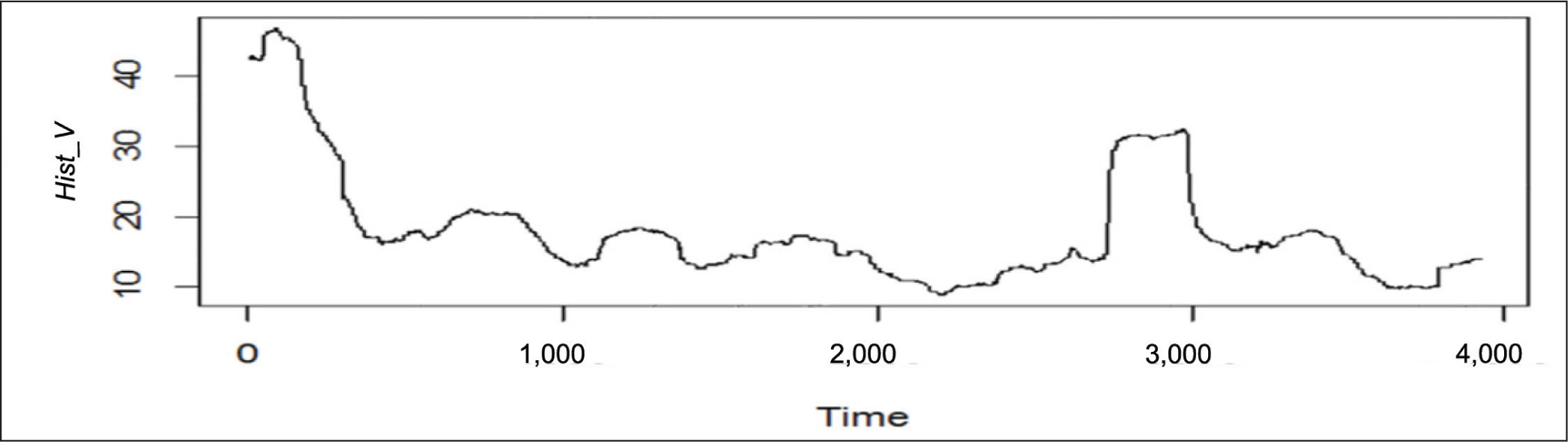
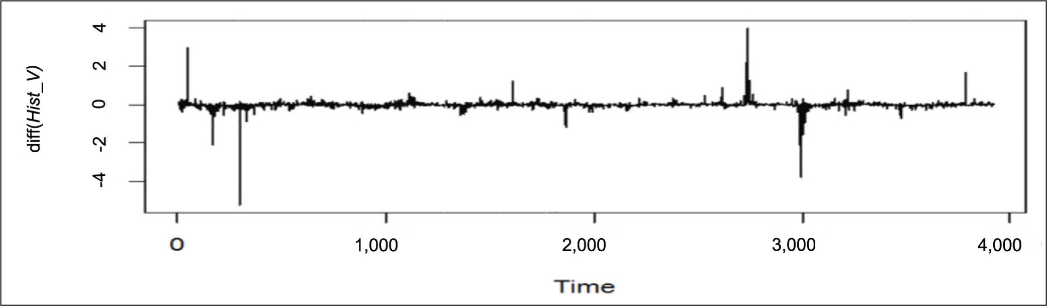
First, we check the presence of stationarity of the time series under study. For checking stationarity, we have used ADF test and KPSS test. ADF test has null hypothesis that the data are not stationary, while KPSS test has the null hypothesis that the data are stationary. The results of unit root testing are given in Table 1. The results of Table 1, in the case of daily data, show that the time series for NIFTY return is stationary at the level, while the time series for historical volatility is stationary at first difference. Figure 1 shows the time series plot of NIFTY returns, while Figures 2 and 3 show the time series plots of historical volatility at level and at first difference.

Table 1.

Unit Root Testing.

Variable	Frequency	ADF Test Statistics	ADF p Value	KPSS Test Statistics	KPSS p Value	Integration Order I(d)
NIFTY returns	Daily	–15.34	.01	0.106	.10	I(0)
Historical volatility	Daily	–2.91	.19	7.54	.01	Not integrated
Historical volatility	Daily at first difference	–10.49	.01	0.59	.20	I(1)

Figure 1.

Daily Log Return.

Figure 2.

Daily Historical Volatility at Level.

Figure 3.

Daily Historical Volatility at First Difference.

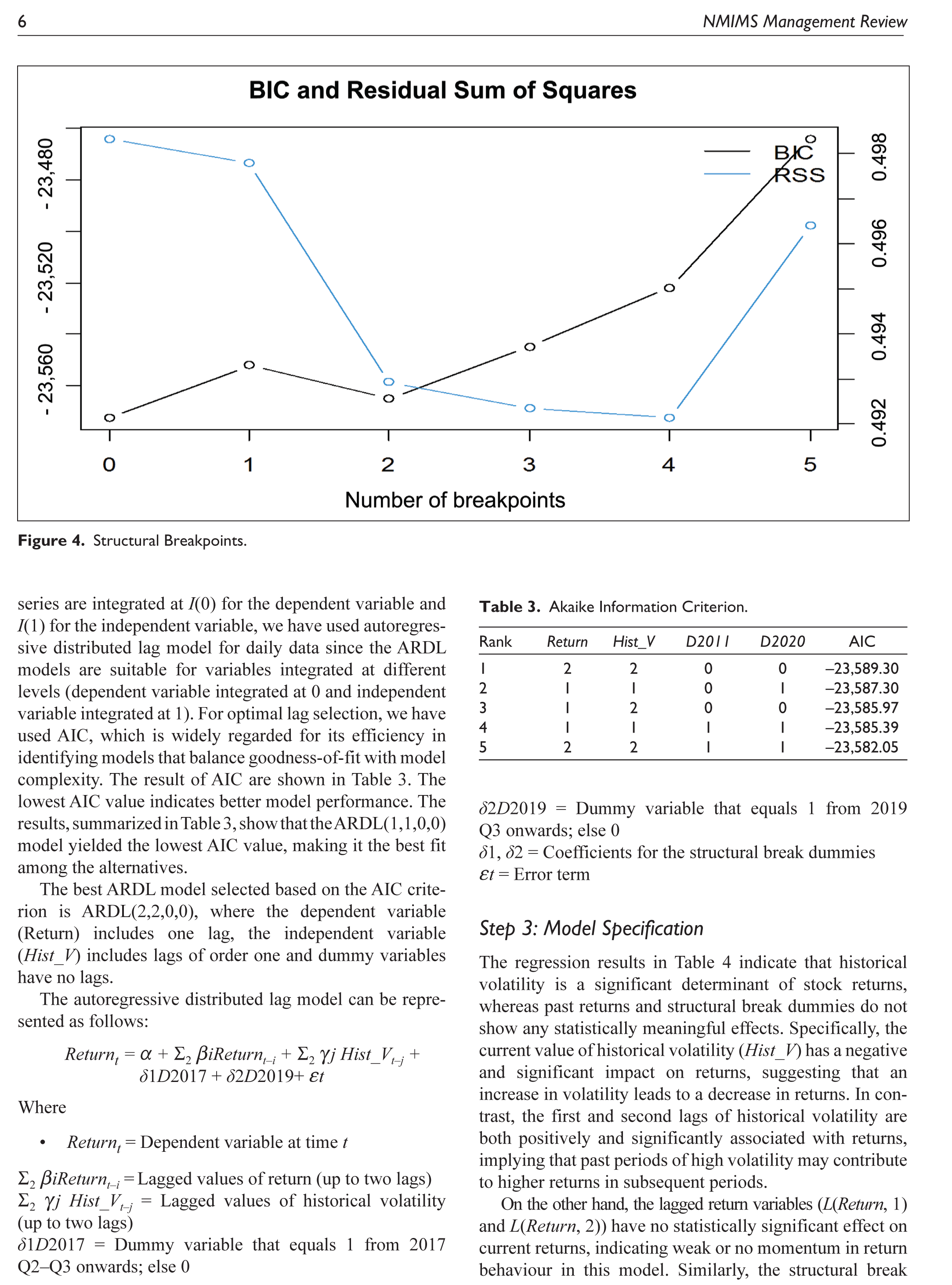
Structural Breakpoints

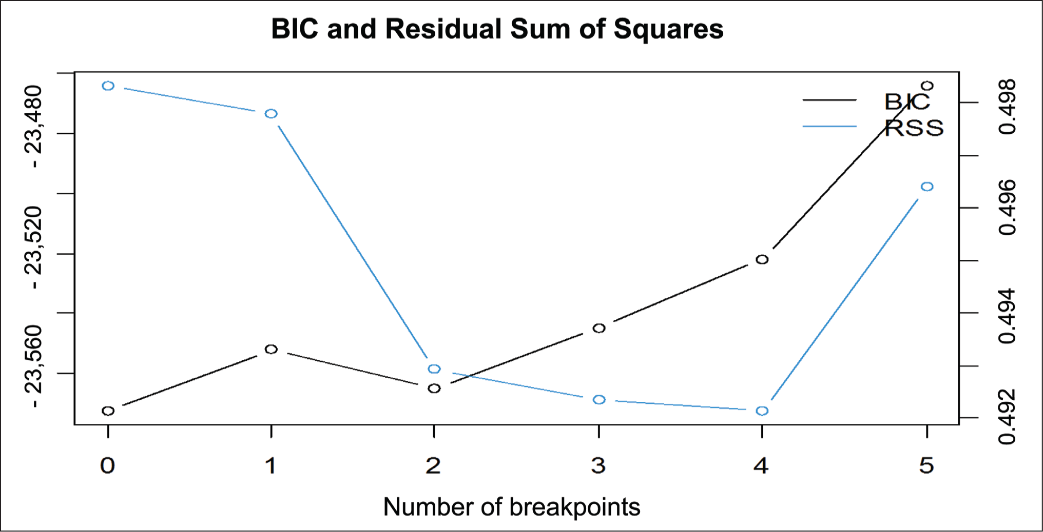
Table 2 shows the results of Bai–Perron test. As per the results, we have taken two breakpoints with minimum BIC, which are the years 2017 and 2019. Figure 4 shows the structural breakpoints in the historical volatility and return. On the x-axis, we observe the number of breakpoints (0–5); on the left y-axis, we have BIC, and on the right y-axis, we have residual sum of squares (RSS). The optimum number of breakpoints are considered when BIC is minimum. In Figure 4, the BIC is minimum at two breakpoints. Thus, the best fitting model, according to BIC, has two structural breaks.

Table 2.

Bai–Perron Test.

Breakpoints (m)	Observations	Approximate Break Dates	BIC
1	584	2011 (Q2–Q3)	–23,040
2	2,151; 2,739	2017 (Q2–Q3), 2019 (Q3)	–23,030
3	584; 2,152; 2,739	2011, 2017, 2019	–23,020
4	584; 1,235; 2,151; 2,739	2011, 2013, 2017, 2019	–23,000
5	584; 1,152; 1,724; 2,298; 2,866	2011, 2013, 2015, 2018, 2020	–22,980

Figure 4.

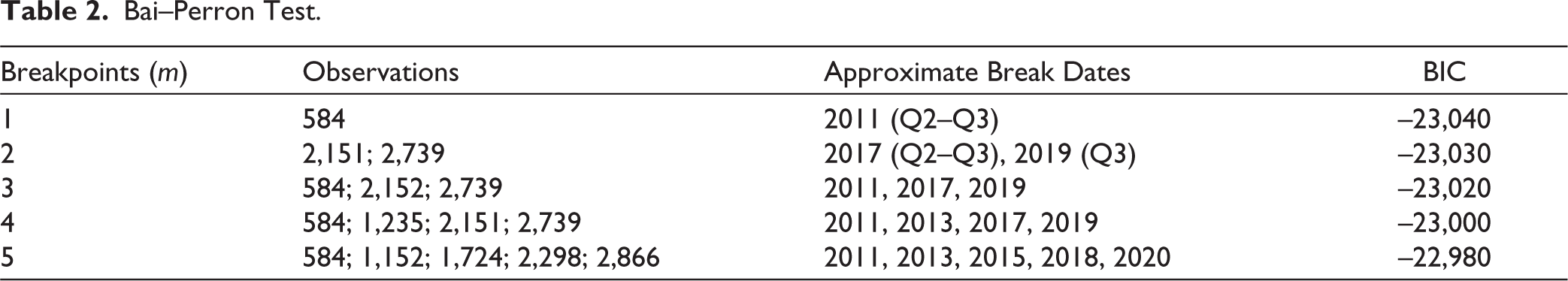
Structural Breakpoints.

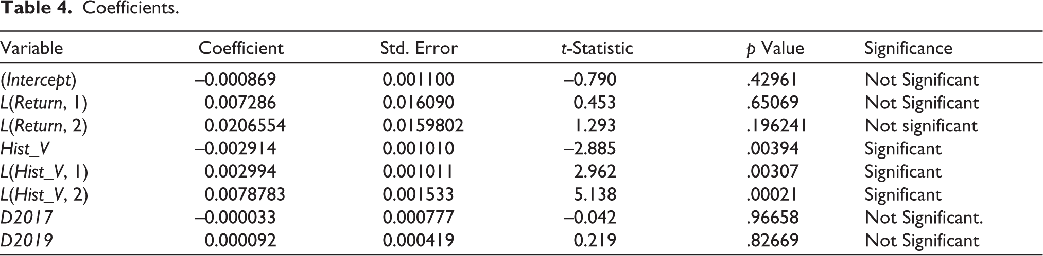
Step 2: Model Identification

We have added two dummy variables D2017 and D2019 for showing the impact of structural break. Since the time series are integrated at I(0) for the dependent variable and I(1) for the independent variable, we have used autoregressive distributed lag model for daily data since the ARDL models are suitable for variables integrated at different levels (dependent variable integrated at 0 and independent variable integrated at 1). For optimal lag selection, we have used AIC, which is widely regarded for its efficiency in identifying models that balance goodness-of-fit with model complexity. The result of AIC are shown in Table 3. The lowest AIC value indicates better model performance. The results, summarized in Table 3, show that the ARDL(1,1,0,0) model yielded the lowest AIC value, making it the best fit among the alternatives.

Table 3.

Akaike Information Criterion.

Rank	Return	Hist_V	D2011	D2020	AIC
1	2	2	0	0	–23,589.30
2	1	1	0	1	–23,587.30
3	1	2	0	0	–23,585.97
4	1	1	1	1	–23,585.39
5	2	2	1	1	–23,582.05

The best ARDL model selected based on the AIC criterion is ARDL(2,2,0,0), where the dependent variable (Return) includes one lag, the independent variable (Hist_V) includes lags of order one and dummy variables have no lags.

The autoregressive distributed lag model can be represented as follows:

Re t u r n_{t} = α + Σ_{2} β i Re t u r n_{t}_{- i} +_{} Σ_{2} γ j H i s t_V_{t}_{- j} + δ_{} 1 D 2017 + δ 2 D 2019 + ε t

Where

Return_t = Dependent variable at time t

Σ₂ βiReturn_t_–i = Lagged values of return (up to two lags)

Σ₂ γj Hist_V_t_–j = Lagged values of historical volatility (up to two lags)

δ1D2017 = Dummy variable that equals 1 from 2017 Q2–Q3 onwards; else 0

δ2D 2019 = Dummy variable that equals 1 from 2019 Q3 onwards; else 0

δ1, δ 2 = Coefficients for the structural break dummies

εt = Error term

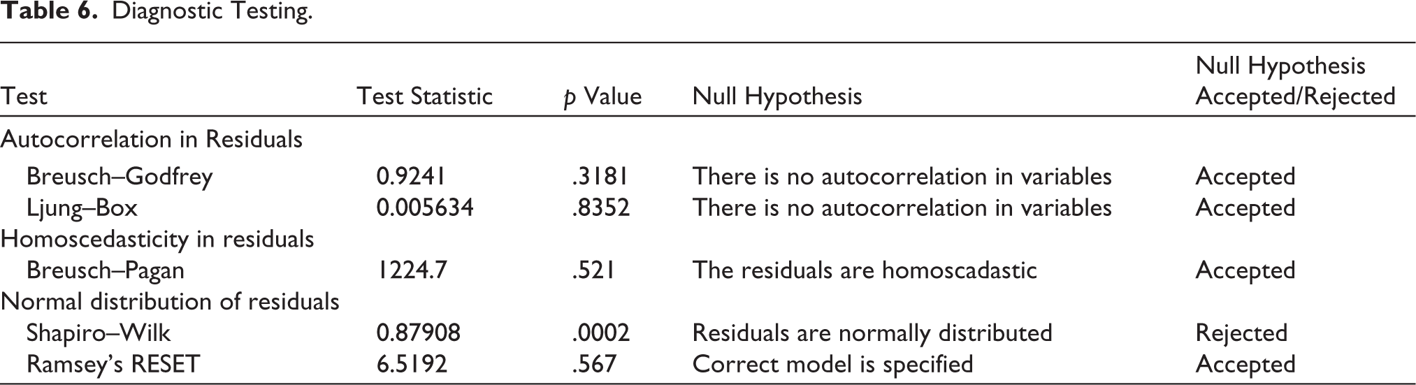
Step 3: Model Specification

The regression results in Table 4 indicate that historical volatility is a significant determinant of stock returns, whereas past returns and structural break dummies do not show any statistically meaningful effects. Specifically, the current value of historical volatility (Hist_V) has a negative and significant impact on returns, suggesting that an increase in volatility leads to a decrease in returns. In contrast, the first and second lags of historical volatility are both positively and significantly associated with returns, implying that past periods of high volatility may contribute to higher returns in subsequent periods.

Table 4.

Coefficients.

Variable	Coefficient	Std. Error	t-Statistic	p Value	Significance
(Intercept)	–0.000869	0.001100	–0.790	.42961	Not Significant
L(Return, 1)	0.007286	0.016090	0.453	.65069	Not Significant
L(Return, 2)	0.0206554	0.0159802	1.293	.196241	Not significant
Hist_V	–0.002914	0.001010	–2.885	.00394	Significant
L(Hist_V, 1)	0.002994	0.001011	2.962	.00307	Significant
L(Hist_V, 2)	0.0078783	0.001533	5.138	.00021	Significant
D2017	–0.000033	0.000777	–0.042	.96658	Not Significant.
D2019	0.000092	0.000419	0.219	.82669	Not Significant

On the other hand, the lagged return variables (L(Return, 1) and L(Return, 2)) have no statistically significant effect on current returns, indicating weak or no momentum in return behaviour in this model. Similarly, the structural break dummy variables for 2017 and 2019 (D2017 and D2019) are statistically insignificant, suggesting that these breakpoints do not have a meaningful impact on the return dynamics within the estimated ARDL framework. Overall, the model highlights the importance of historical volatility—particularly its lagged values—in explaining return variations, while past returns and structural breaks appear to play a limited role.

The model explains only a small portion of the variation in returns, as indicated by the low R² value (0.0059). However, the overall model is statistically significant, with an F-statistic of 4.571 and a p value of .00037, suggesting that the included variables jointly have explanatory power.

ARDL Bound Test

The results of the bound test in Table 5 indicate a very high F-statistic of 951.76 with a p value of 1e-06, which is far above any conventional upper critical bound. This provides strong statistical evidence to reject the null hypothesis of no cointegration. Therefore, we conclude that a long-run equilibrium relationship exists between the dependent variable (Return) and the explanatory variables (Hist_V, D2017 and D2019).

Table 5.

Bound F-test for Cointegration.

Statistic	Value
F	951.76
p value	1e-06
Decision	Reject null of no cointegration

Step 4: Diagnostic Testing

The results of diagnostic testing are summarized in Table 6 and provide key insights into the validity of the regression model. To examine autocorrelation in the residuals, both the Breusch–Godfrey and Ljung–Box tests were applied. The Breusch–Godfrey test yielded a statistic of 0.9241 with a p value of .3181, and the Ljung–Box test produced a χ² value of 0.005634 with a p value of .8352. In both cases, the null hypothesis of no serial correlation was accepted, indicating that there is no serial correlation in the residuals. For heteroscedasticity, the Breusch–Pagan test was conducted. It returned a test statistic of 1,224.7 with a p value of 0.521, suggesting that the null hypothesis of homoscedasticity cannot be rejected. This means that the residuals exhibit constant variance, satisfying an important assumption of regression analysis.

Table 6.

Diagnostic Testing.

Test	Test Statistic	p Value	Null Hypothesis	Null Hypothesis Accepted/Rejected
Autocorrelation in Residuals
Breusch–Godfrey	0.9241	.3181	There is no autocorrelation in variables	Accepted
Ljung–Box	0.005634	.8352	There is no autocorrelation in variables	Accepted
Homoscedasticity in residuals
Breusch–Pagan	1224.7	.521	The residuals are homoscadastic	Accepted
Normal distribution of residuals
Shapiro–Wilk	0.87908	.0002	Residuals are normally distributed	Rejected
Ramsey’s RESET	6.5192	.567	Correct model is specified	Accepted

The Shapiro–Wilk test was used to assess the normality of residuals. The test statistic was 0.87908, with a p value of .0002, leading to a rejection of the null hypothesis. This indicates that the residuals are not normally distributed. While this could influence inference in smaller samples, it is generally less problematic in large samples due to the central limit theorem. Ramsey’s RESET test was used to evaluate the model specification. The test yielded a statistic of 6.5192 with a p value of .567, supporting the acceptance of the null hypothesis that the model is correctly specified. This indicates that the chosen functional form of the model is appropriate and well-fitted to the data.

In summary, the diagnostic tests confirm that the model meets essential assumptions of no autocorrelation, homoscedasticity and correct specification. Although the residuals are not normally distributed, the model remains statistically robust, especially in the context of a large sample.

Implications

This study is relevant for a wide range of market participants and stakeholders including investors, portfolio managers, academic researchers and policymakers. The study of historical trends and their correlation with NIFTY returns will help stakeholders understand the long-term market trends and develop informed strategies (Hingane et al., 2023). The study will provide policymakers with insights into the market stability and economic linkages that affect stock market performance. This can help portfolio managers fine-tune their risk management and asset allocation. Academic researchers can use this to base predictive models of market returns using historical data.

Conclusion

Literature on historical volatility and stock market returns provides substantial evidence that market fluctuations influence future price movements, specifically in emerging markets like India. While traditional financial theories argue against predictability, empirical studies state that historical volatility impacts investor sentiment, risk perception and trading behaviour. Understanding the historical pattern and their correlation with NIFTY returns, the current research provides valuable implication for stakeholders. The research shows both short- and long-run relationship between the variables. The ARDL bound test confirmed a statistically significant long-run cointegrating relationship between historical volatility and NIFTY returns, reinforcing the model’s validity. The diagnostic testing of the model also validates the robustness of the model.

The existing literature on historical volatility and NIFTY returns has deeply examined the behaviour of return fluctuations in the Indian stock market using various econometric models. A significant number of studies have employed GARCH-type models to understand volatility clustering, persistence and mean reversion in NIFTY returns (Mahajan et al., 2022; Parasuraman & Ramudu, 2011). These studies largely focus on short- to medium-term data and emphasize daily or intra-day returns to analyse volatility dynamics. Several works also highlight the tendency of historical volatility to revert to the mean and the existence of volatility spillovers between implied and historical measures (Mishra et al., 2025). The findings consistently suggest that while historical volatility helps in understanding past market behaviour, implied volatility often serves as a better forward-looking measure (Chakrabarti & Kumar, 2020; Padhi & Shaikh, 2014). Some studies have found clear evidence of volatility persistence in NIFTY returns, indicating that volatility shocks tend to have prolonged effects. Despite these robust insights, the majority of existing research does not incorporate the role of structural changes or long-term regime shifts in volatility behaviour. The present study has included the structural changes in the very long run.

This gap is particularly notable as most studies have examined volatility in isolation from broader economic or policy-driven transformations, with only limited attention to large-scale events such as demonetization (Raj & Pandikumar, 2017). In contrast, our study spans a much longer period—from 2009 to 2025—and explicitly accounts for structural breaks, allowing it to capture key shifts in the volatility–return relationship across different economic regimes. By identifying breakpoints in volatility trends, our work provides a more nuanced and temporally sensitive understanding of NIFTY return dynamics, something that earlier works with shorter time spans or static models could not fully achieve. In doing so, our research fills an important gap in the literature and offers a more holistic view of volatility behaviour in evolving market contexts.

Footnotes

Declaration of Conflicting Interests

The authors declared no potential conflicts of interest with respect to the research, authorship and/or publication of this article.

Funding

The authors received no financial support for the research, authorship and/or publication of this article.

References

Ali

S. E. A.

, Lai

F.-W.

, Hassan

, & Shad

M. K.

(2021). The Long-run impact of information security breach announcements on investors’ confidence: The context of efficient market hypothesis. Sustainability, 13(3), 1066. https://doi.org/10.3390/su13031066

Alkhatib

, Khazaleh

, Alkhazaleh

H. A.

, Alsoud

A. R.

, & Abualigah

(2022). A new stock price forecasting method using active deep learning approach. Journal of Open Innovation: Technology, Market, and Complexity, 8(2), 96. https://doi.org/10.3390/joitmc8020096

Awan

, Shamim

, Khan

, Zia

N. U.

, Shariq

S. M.

, & Khan

M. N.

(2021). Big data analytics capability and decision-making: The role of data-driven insight on circular economy performance. Technological Forecasting and Social Change, 168, 120766. https://doi.org/10.1016/j.techfore.2021.120766

Bai

, & Perron

(2003). Computation and analysis of multiple structural change models. Journal of Applied Econometrics, 18(1), 1–22.

Baker

, & Wurgler

(2007). Investor sentiment in the stock market. Journal of Economic Perspectives, 21(2), 129–151. https://doi.org/10.1257/jep.21.2.129

Banz

R. W.

(1981). The relationship between return and market value of common stocks. Journal of Financial Economics, 9(1), 3–18. https://doi.org/10.1016/0304-405X(81)90018-0

Beloskar

V. D.

, & Nageswara Rao

S. V. D.

(2024). Screening activity matters: Evidence from ESG portfolio performance from an emerging market. International Journal of Finance & Economics, 29(3), 2593–2619. https://doi.org/10.1002/ijfe.2798

Ben Osman

, Galariotis

, Guesmi

, Hamdi

, & Naoui

(2024). Are markets sentiment driving the price bubbles in the virtual? International Review of Economics & Finance, 89, 272–285. https://doi.org/10.1016/j.iref.2023.10.041

Borges

, Maia

, & Guerreiro

(2024). Forecasting electricity price during extreme events using a hybrid model of LSTM and ARIMA architecture. In Filipe

, Śmiałek

, Brodsky

, & Hammoudi

(Eds), Enterprise information systems (Vol. 518, pp. 310–329). Springer Nature. https://doi.org/10.1007/978-3-031-64748-2_15

10.

Bouri

, & Harb

(2022). The size of good and bad volatility shocks does matter for spillovers. Journal of International Financial Markets, Institutions and Money, 80, 101626. https://doi.org/10.1016/j.intfin.2022.101626

11.

Chakrabarti

, & Kumar

K. K.

(2020). High-frequency return-implied volatility relationship: Empirical evidence from NIFTY and India VIX. The Journal of Developing Areas, 54(3). https://doi.org/10.1353/jda.2020.0024

12.

Chakraborty

, & Parida

(2024). Comprehensive study of AI-driven market forecasting models and their applicability. 2024 International Conference on Advancements in Smart, Secure and Intelligent, Computing (ASSIC), 1–5. https://doi.org/10.1109/ASSIC60049.2024.10508015

13.

Chandra

(2012). Cause and effect between FII trading behaviour and stock market returns: The Indian experience. Journal of Indian Business Research, 4(4), 286–300. https://doi.org/10.1108/17554191211274794

14.

Chang

, & Tsai

(2008). Forecast approach using neural network adaptation to support vector regression grey model and generalized auto-regressive conditional heteroscedasticity. Expert Systems with Applications, 34(2), 925–934. https://doi.org/10.1016/j.eswa.2006.10.034

15.

Chu

, He

X.-Z.

, Li

, & Tu

(2022). Investor sentiment and paradigm shifts in equity return forecasting. Management Science, 68(6), 4301–4325. https://doi.org/10.1287/mnsc.2020.3834

16.

Dongrey

(2022). Study of market indicators used for technical analysis. International Journal of Engineering and Management Research, 12(2), 64–83. https://doi.org/10.31033/ijemr.12.2.11

17.

Durham

G. R.

, Hertzel

M. G.

, & Martin

J. S.

(2005). The market impact of trends and sequences in performance: New evidence. The Journal of Finance, 60(5), 2551–2569. https://doi.org/10.1111/j.1540-6261.2005.00807.x

18.

Engle

(2004). Risk and volatility: Econometric models and financial practice. American Economic Review, 94(3), 405–420. https://doi.org/10.1257/0002828041464597

19.

Goetzmann

W. N.

, Ibbotson

R. G.

, & Peng

(2001). A new historical database for the NYSE 1815 to 1925: Performance and predictability. Journal of Financial Markets, 4(1), 1–32. https://doi.org/10.1016/S1386-4181(00)00013-6

20.

Gomes

, & Gubareva

(2021). Complex systems in economics and where to find them. Journal of Systems Science and Complexity, 34(1), 314–338. https://doi.org/10.1007/s11424-020-9149-1

21.

Hingane

, Ukhalkar

, Bhate

, & Hingane

(2023). Study of various approaches and prediction models for Indian stock market with reference to NIFTY50 index. 2023 7th International Conference on Computing, Communication, Control and Automation (ICCUBEA), 1–6. https://doi.org/10.1109/ICCUBEA58933.2023.10392010

22.

Huber

, Huber

, & Kirchler

(2022). Volatility shocks and investment behavior. Journal of Economic Behavior & Organization, 194, 56–70. https://doi.org/10.1016/j.jebo.2021.12.007

23.

Huy

D. T. N.

, Nhan

V. K.

, Bich

N. T. N.

, Hong

N. T. P.

, Chung

N. T.

, & Huy

P. Q.

(2021). Impacts of internal and external macroeconomic factors on firm stock price in an expansion econometric model: A case in Vietnam real estate industry. In Thach

N. Ngoc

, Kreinovich

, & Trung

N. D.

(Eds), Data science for financial econometrics (Vol. 898, pp. 189–205). Springer International Publishing. https://doi.org/10.1007/978-3-030-48853-6_14

24.

Kahn

R. N.

, & Rudd

(1995). Does historical performance predict future performance? Financial Analysts Journal, 51(6), 43–52. https://doi.org/10.2469/faj.v51.n6.1948

25.

Kashyap

(2023). Review on volatility and return analysis including emerging developments: Evidence from stock market empirics. Journal of Modelling in Management, 18(3), 756–816. https://doi.org/10.1108/JM2-10-2021-0249

26.

Kaur

(2018). Securities market in India: Regulation of undesirable practices by the Securities and Exchange Board of India. In Bian

& Çalıyurt

K. T.

(Eds), Regulations and applications of ethics in business practice (pp. 273–293). Springer. https://doi.org/10.1007/978-981-10-8062-3_15

27.

Klos

, Weber

E. U.

, & Weber

(2005). Investment decisions and time horizon: Risk perception and risk behavior in repeated gambles. Management Science, 51(12), 1777–1790. https://doi.org/10.1287/mnsc.1050.0429

28.

Kumar

, Jain

, & Singh

U. P.

(2021). Stock market forecasting using computational intelligence: A survey. Archives of Computational Methods in Engineering, 28(3), 1069–1101. https://doi.org/10.1007/s11831-020-09413-5

29.

Lee

W. Y.

, Jiang

C. X.

, & Indro

D. C.

(2002). Stock market volatility, excess returns, and the role of investor sentiment. Journal of Banking & Finance, 26(12), 2277–2299. https://doi.org/10.1016/S0378-4266(01)00202-3

30.

Locke

, & Gupta

(2009). Applicability of contrarian strategy in the Bombay Stock Exchange. Journal of Emerging Market Finance, 8(2), 165–189. https://doi.org/10.1177/097265270900800204

31.

Lundblad

(2007). The risk return tradeoff in the long run: 1836–2003. Journal of Financial Economics, 85(1), 123–150. https://doi.org/10.1016/j.jfineco.2006.06.003

32.

Mahajan

, Thakan

, & Malik

(2022). Modelling and forecasting the volatility of NIFTY 50 using GARCH and RNN models. Economies, 10(5), 102.

33.

Malkiel

B. G.

(1989). Efficient market hypothesis. In Eatwell

, Milgate

, & Newman

(Eds), Finance (pp. 127–134). Palgrave Macmillan. https://doi.org/10.1007/978-1-349-20213-3_13

34.

Malkiel

B. G.

(2003). The efficient market hypothesis and its critics. Journal of Economic Perspectives, 17(1), 59–82. https://doi.org/10.1257/089533003321164958

35.

Megaravalli

A. V.

, & Sampagnaro

(2018). Macroeconomic indicators and their impact on stock markets in ASIAN 3: A pooled mean group approach. Cogent Economics & Finance, 6(1), 1432450. https://doi.org/10.1080/23322039.2018.1432450

36.

Merton

R. C.

(1980). On estimating the expected return on the market. Journal of Financial Economics, 8(4), 323–361. https://doi.org/10.1016/0304-405X(80)90007-0

37.

Mishra

B. B.

, Sahay

, & Sharma

(2025). Investigating the spillover effect of implied volatility on NIFTY return in different time periods with reference to index options: A multivariate GARCH approach. International Journal of System Assurance Engineering and Management. https://doi.org/10.1007/s13198-025-02711-w

38.

Muguto

, & Muzindutsi

P.-F.

(2022). A comparative analysis of the nature of stock return volatility in BRICS and G7 markets. Journal of Risk and Financial Management, 15(2), 85. https://doi.org/10.3390/jrfm15020085

39.

Mukherjee

, & Roy

(2016). What drives the stock market return in India? An exploration with dynamic factor model. Journal of Emerging Market Finance, 15(1), 119–145. https://doi.org/10.1177/0972652715623681

40.

Mukherjee

, & Mandal

(2024). Impact of market volatility on NIFTY 50 returns: An empirical study. SSRN Electronic Journal. https://doi.org/10.2139/ssrn.4964444

41.

Nkoro

, & Uko

A. K.

(2016). Autoregressive distributed lag (ARDL) cointegration technique: Application and interpretation. Journal of Statistical and Econometric Methods, 5(4), 63–91.

42.

Ospina

, Gondim

J. A. M.

, Leiva

, & Castro

(2023). An overview of forecast analysis with ARIMA models during the COVID-19 pandemic: Methodology and case study in Brazil. Mathematics, 11(14), 3069. https://doi.org/10.3390/math11143069

43.

Padhi

, & Shaikh

(2014). On the relationship of implied, realized and historical volatility: Evidence from NSE equity index options. Journal of Business Economics and Management, 15(5), 915–934.

44.

Pandey

, & Sehgal

(2016). Explaining size effect for Indian stock market. Asia-Pacific Financial Markets, 23(1), 45–68. https://doi.org/10.1007/s10690-015-9208-0

45.

Parasuraman

N. R.

, & Ramudu

P. J.

(2011). Historical and implied volatility: An investigation into NSE NIFTY futures and options. Australian Journal of Business and Management Research, 1(7), 112.

46.

Pillai

(2023). Integrating AI-driven techniques in big data analytics: Enhancing decision-making in financial markets. International Journal of Engineering and Computer Science, 12(7), 25774–25788. https://doi.org/10.18535/ijecs/v12i07.4745

47.

Poitras

(2012). From the renaissance exchanges to cyberspace: A history of stock market globalization. In Poitras

(Ed.), Handbook of research on stock market globalization. Edward Elgar Publishing. https://doi.org/10.4337/9780857938183.00012

48.

Poon

S.-H.

, & Granger

C. W. J.

(2003). Forecasting volatility in financial markets: A review. Journal of Economic Literature, 41(2), 478–539. https://doi.org/10.1257/jel.41.2.478

49.

Raj

, & Pandikumar

M. P.

(2017). Historical volatility of NIFTY returns and demonetisation: An overview. Sumedha Journal of Management, 6(2), 4–21.

50.

Raza

H. M. Z.

, Haider

, & Haider

S. Z.

(2024). Forecasting stock prices: Exploring the potential of ARIMA model for short-term predictions. International Journal of Management Research and Emerging Sciences, 14(4). https://doi.org/10.56536/ijmres.v14i4.654

51.

Rosenberg

, Reid

, & Lanstein

(1998). Persuasive evidence of market inefficiency (spring 1985). In Bernstein

P. L.

& Fabozzi

F. J.

(Eds), Streetwise (pp. 48–55). Princeton University Press. https://doi.org/10.1515/9781400829408-007

52.

Sabarinathan

(2010). SEBI’s regulation of the Indian securities market: A critical review of the major developments. Vikalpa: The Journal for Decision Makers, 35(4), 13–26. https://doi.org/10.1177/0256090920100402

53.

Sahu

T. N.

(Ed.). (2015). The Indian Stock Market and the macroeconomic environment: An overview. In Macroeconomic variables and security prices in India during the liberalized period (pp. 11–38). Palgrave Macmillan. https://doi.org/10.1057/9781137492012_2

54.

Sarkodie

S. A.

, & Owusu

P. A.

(2020). How to apply the novel dynamic ARDL simulations (DYNARDL) and Kernel-based regularized least squares (KRLS). MethodsX, 7, 101160.

55.

Schwert

G. W.

(1989). Why does stock market volatility change over time? The Journal of Finance, 44(5), 1115–1153. https://doi.org/10.1111/j.1540-6261.1989.tb02647.x

56.

Shah

, Isah

, & Zulkernine

(2019). Stock market analysis: A review and taxonomy of prediction techniques. International Journal of Financial Studies, 7(2), 26. https://doi.org/10.3390/ijfs7020026

57.

Shah

, Vaidya

, & Shah

(2022). A comprehensive review on multiple hybrid deep learning approaches for stock prediction. Intelligent Systems with Applications, 16, 200111. https://doi.org/10.1016/j.iswa.2022.200111

58.

Shiller

R. J.

(2003). From efficient markets theory to behavioral finance. Journal of Economic Perspectives, 17(1), 83–104. https://doi.org/10.1257/089533003321164967

59.

Snowden

K. A.

(1990). Historical returns and security market development, 1872–1925. Explorations in Economic History, 27(4), 381–420. https://doi.org/10.1016/0014-4983(90)90022-Q

60.

Subburayan

(2017). An empirical study on influence of economic fundamentals on Indian Stock Market. SSRN Electronic Journal. https://doi.org/10.2139/ssrn.3748921

61.

Toromade

A. S.

, & Chiekezie

N. R.

(2024). Forecasting stock prices and market trends using historical data to aid investment decisions. Finance & Accounting Research Journal, 6(8), 1472–1484. https://doi.org/10.51594/farj.v6i8.1434

62.

Waghela

, Sen

, & Rakshit

(2024). A performance analysis of technical indicators on the Indian Stock Market. In Pedrycz

, Rivera

, Fernández

, & Meschino

G. J.

(Eds), Artificial intelligence in prescriptive analytics (Vol. 260, pp. 451–495). Springer Nature. https://doi.org/10.1007/978-3-031-66731-2_18

63.

Xiuzhen

, Zheng

, & Umair

(2022). Testing the fluctuations of oil resource price volatility: A hurdle for economic recovery. Resources Policy, 79, 102982. https://doi.org/10.1016/j.resourpol.2022.102982

64.

Yang

(2024). Pandemic, policy, and markets: Insights and learning from COVID-19’s impact on global stock behavior. Empirical Economics. https://doi.org/10.1007/s00181-024-02648-2

65.

Yurttagüler

İ.

(2024). Analysis of BIST gold index volatility with autoregressive conditional heteroscedasticity models. İnsan ve Toplum Bilimleri Araştırmaları Dergisi, 13(3), 1256–1276. https://doi.org/10.15869/itobiad.1390321

66.

Zhong

, & Enke

(2019). Predicting the daily return direction of the stock market using hybrid machine learning algorithms. Financial Innovation, 5(1), 24. https://doi.org/10.1186/s40854-019-0138-0

Historical Volatility and NIFTY Returns: A Multi-timeframe Analysis Using ARDL Models

Abstract

Keywords

Introduction

Origin of Financial Market and Importance of Historical Data

Understanding NIFTY Returns

Literature Review

Theoretical Background and Divergent Views on Volatility and Returns

Empirical Studies Supporting the Predictive Power of Historical Volatility

Empirical Studies Challenging the Predictive Role of Historical Volatility

Empirical Approaches for Analysing and Modelling of Historical Volatility and NIFTY Returns

Research Methodology

Data

The Econometric Research Methods

Data Analysis and Interpretation

Step 1: Unit Root Test

Daily Log Return.

Daily Historical Volatility at Level.

Daily Historical Volatility at First Difference.

Structural Breakpoints

Structural Breakpoints.

Step 2: Model Identification

Step 3: Model Specification

ARDL Bound Test

Step 4: Diagnostic Testing

Implications

Conclusion

Footnotes

Declaration of Conflicting Interests

Funding

References