Sage Journals: Discover world-class research

Abstract

The aim of the present work is to apply the Larson–Miller technique for the study of the mechanical behavior under creep of high-modulus polyethylene (HMPE) fibers focused on use as in offshore mooring ropes. Creep is known to be a long-term phenomenon, so in most cases, reproducing such experiments in real time is not feasible, and as the life span of anchoring systems must be in the order of decades, accelerated tests are required to verify the long-term mechanical behavior of the material. The methodology using the Larson–Miller parameter is a well-documented and powerful technique for materials’ lifetime prediction, although seldom applied to polymeric materials. It involves in performing accelerated (high temperature and/or loads) creep tests to determine the parameters that are later used to estimate the rupture time of the material under constant load. It is concluded that the Larson–Miller technique is efficient for calculating the lifetime of HMPE subjected to creep.

Keywords

Larson–Miller synthetic fibers high-modulus polyethylene creep mooring

Introduction

Oil and gas exploitation in deep and ultra-deepwater has increased over the past decades, as new fields are discovered in the salt and pre-salt layers, where the water depth is in the order of thousands of meters.^1,2 Operationally, the design of important equipment used in offshore platforms working in this new scenario, such as risers, umbilicals, and mooring ropes, had to be rethought to fulfill safety and efficiency requirements in these new, more severe service conditions.

In terms of mooring systems, in the past, they used to be traditionally based on steel wire ropes and chains. However, with the substantial increase in water depth, these metallic components would become long enough to the point that their self-weight might exceed the platform’s floating forces.1 This picture has pushed the oil and gas industry into considering the application of different, lighter classes of materials to the mooring systems, and polymers were considered as a viable choice.

Along the past three decades, extensive research was done with different materials, studying different mechanical properties. An interesting overview of different examples of synthetic mooring ropes, including several materials and properties, can be found in the literature,^3

–6 and general guidance and recommendations regarding these systems can be found in the literature.^7
–9 More specifically, studies dealing with long-term behavior of fibers under constant tension, that is, creep, are of utmost importance when it comes to mooring systems. In that sense, theoretical models have been proposed in the literature for several distinct materials, whose results are found in the literature.^10

–16

During the lifetime of a mooring rope, it is constantly subjected to time-varying, nonzero mechanical tensile loading due to a complex combination of self-weight, waves, ocean current, wind acting on the platform, and so on. The fact that this tensile load is always positive and larger than or equal to the rope’s self-weight leads to the necessity of assessing the mechanical behavior of the rope’s materials under creep, especially because it is a long-term effect much more accentuated in polymers than it is in metals and might eventually cause premature failure of the structure.

The mechanical properties of high-modulus polyethylene (HMPE) fibers make them suitable to be used in applications where high stiffness and tensile strength are required along with low elongation, mainly due to its high level of crystallinity (up to 85%) and fiber orientation (greater than 95%). It shows good fatigue and abrasion resistance, ultimate strength and stiffness similar to those of low carbon steel, and density lower than 1000 kg/m³, therefore lighter than water.^17,18 All these properties make HMPE a suitable type of material to be used in offshore mooring ropes. However, even though it shows higher tensile strength and lower density than polyester^19,20 (most common material used in mooring ropes), unlike the latter, which do not show significant creep in service conditions of mooring systems, the former tends to present a more accentuated creep behavior at the same conditions (strongly dependent on material grade). It is, therefore, mandatory to assess such mechanical behavior when one is considering using HMPE in mooring applications.

However, the long-term nature of creep makes it prohibitive to perform real-time experiments, thus the use of accelerating techniques is highly recommended. Generally, when dealing with polymeric materials, temperature can be used as a key variable to accelerate the mechanical response being evaluated, and correlation/extrapolation techniques are later used to verify the long-term response of a chosen parameter at lower temperatures.

The goal of this article is thus to apply the Larson–Miller methodology²¹ determining the validity of its use as a predictor of the lifetime of HMPE yarns subjected to creep at operational temperatures. The tests were performed in three different load levels and six temperatures, allowing the calculation of the Larson–Miller parameter (LMP) for the material. Then, it was possible to predict the lifetime of HMPE under creep at any chosen tensile load exposed to any chosen temperature.

Larson–Miller methodology: Theoretical background and use

The Larson–Miller methodology uses an Arrhenius-like equation and provides results for creep life span at any desired load level at any desired temperature. Prior to its application, however, it is necessary to compute the LMP for a given load level according to

LMP = T \frac{(C + log t_{f})}{1000}

where T is the test temperature (K), C is a material parameter, and t_f is the overall time (h) until the sample fails by creep at temperature T.

For the determination of the parameter C, it is thus required to perform at least two creep experiments at a fixed load level and two different temperatures, so one can plot the graph of log(t_f) versus 1/T and fit a linear curve to the points acquired. Parameter C is then the point where the fitted curve intercepts the vertical axis log(t_f) (Figure 1).

Figure 1.

Experimental determination of the parameter C.

Equation (1) is used to calculate the LMP for that particular load level tested and then used again to determine the lifetime under creep (t_f) for that same load level, but at any temperature T. Although the parameter C is often considered a material constant for metals, that is, independent of the load level tested, in this article, it was found that, for HMPE, it has a considerable dependency on the creep load and, therefore, is going to be treated as a variable.

Material and methods

Material

All the experiments were performed in DSM Dyneema DM20^® (Heerlen, Netherlands) HMPE yarn samples, which have a linear density of 1760 dtex, tensile strength of 3.1 GPa, and tensile modulus of 93 GPa. Its use in mooring ropes of offshore platforms is one among its many possible commercial applications.

Tensile tests

To determine the load plateaus for the creep experiments, it was mandatory to determine the tensile strength of the HMPE yarns, also called yarn break load (YBL) of the material. For such, 30 rupture tests were performed in 500-mm long yarn samples of HMPE under the displacement control of 250 mm/min according to ASTM D2256.²² The samples were twisted along their axes with 60 rounds per meter. An Instron 3365 (Norwood, U.S.) universal testing machine with a ±1-kN load cell was used.

Creep tests

The creep experiments were performed in an Instron 5969 universal testing machine with a ±10-kN load cell with a temperature chamber attached. Due to the high elongation of the samples during high-temperature creep tests, the samples used were 250-mm long, also with a torsion of 60 rounds per meter. Table 1 resumes the load and temperature levels tested. All the experiments were performed up to the rupture of the samples.

Table 1.

Overview of the load levels and temperatures of the creep experiments.

Load level (% YBL)	Temperature (°C)
40	40, 50, 60, 80, and 100
50	40, 50, 60, 80, and 100
70	40, 50, 60, 70, and 80

YBL: yarn break load.

At 100°C, the samples tested at 70% YBL failed (rupture) before initiating the constant load plateau, so a new temperature level of 70°C was considered to keep all the load levels exposed to the same number of temperature levels.

Results and discussion

As mentioned in the “Tensile tests” section, a series of 30 tensile tests was performed and the YBL of HMPE was determined as being 487.5 N. Figure 2 shows the creep curves for each case of Table 1, and Figure 3 resumes them with both experimental data and the linear curve fitted to each load level, to obtain parameter C. As mentioned in the “Larson–Miller methodology: Theoretical background and use” section, C was found not to be a constant for HMPE, as usually considered for metallic materials. For that reason, it was treated as dependent on the load level tested during each creep experiment.

Figure 2.

Creep curves of the experiments presented in Table 1: (a) 40% YBL at 40°C; (b) 50% YBL at 40°C; (c) 70% YBL at 40°C; (d) 40% YBL at 50°C; (e) 50% YBL at 50°C; (f) 70% YBL at 50°C; (g) 40% YBL at 60°C; (h) 50% YBL at 60°C; (i) 70% YBL at 60°C; (j) 40% YBL at 80°C; (k) 50% YBL at 80°C; (l) 70% YBL at 70°C; (m) 40% YBL at 100°C; (n) 50% YBL at 100°C; (o) 70% YBL at 80°C.

Figure 3.

Experimental data of t_f versus 1/T for each particular load level, together with linear curves fitted.

The linear regression coefficients in Figure 3 show a highly linear correlation between the test temperature T and the lifetime under creep t_f for each particular load level, considering the grade of HMPE tested. This observation is important as it can be used as future reference while planning experimental setups for different grades of HMPE, making it possible to reduce it to only two or three creep tests, which is sufficient to determine accurate linear curves to fit the experimental data. Table 2 presents the main results as shown in Figure 3.

Table 2.

Lifetime under creep load and parameter C for the load and temperature levels.

	Temperature (°C)						Parameter C
	40	50	60	70	80	100	Parameter C
t_f (h)
40% YBL	180.78	36.13	8.55	–	0.6781	0.0415	20.06
50% YBL	27.50	7.45	1.44	–	0.1628	0.0048	21.31
70% YBL	1.75	0.6165	0.0944	0.0439	0.0035	–	22.60

YBL: yarn break load.

The LMP for each load and temperature level is computed using equation (1), whose results are presented in Table 3.

Table 3.

Larson–Miller parameter for each load level.

	Temperature (°C)	LMP	Average LMP
40% YBL	40	6.9883	6.9922
	50	6.9855
	60	6.9932
	80	7.0243
	100	6.9693
50% YBL	40	7.1243	7.1561
	50	7.1685
	60	7.1526
	80	7.2476
	100	7.0865
70% YBL	40	7.1520	7.1951
	50	7.2340
	60	7.1863
	70	7.2881
	80	7.1142

LMP: Larson–Miller parameter; YBL: yarn break load.

The conclusion that the parameter C is not constant for HMPE leads to a different approach of the classical Larson–Miller methodology, because C—and consequently LMP—will need to be recalculated to determine the creep lifetime for an arbitrary load level that was not previously tested. The calculation of C and LMP in this case can be made by linear regressions of the already obtained C and LMP presented in Tables 2 and 3, respectively (Figure 4).

Figure 4.

Determination of (a) C and (b) LMP for different—not tested—load levels.

By rearranging the terms in equation (1), one can determine the lifetime prediction t_f (h) of HMPE under creep, subjected to a chosen load level, at temperature T (K) using equation (2), having calculated C and LMP according to the linear regressions of Figure 4(a) and (b), respectively

t_{f} = 10^{(1000 \frac{LMP}{T} - C)}

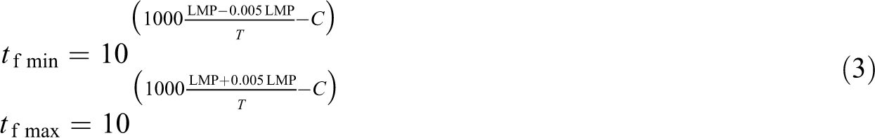
Due to the logarithmic nature of the relation depicted in equation (2), very small changes in any of the variables in the right-hand side of the equation lead to considerable changes in the overall lifetime t_f. For that reason, to account for experimental variability and inaccuracy of the linear regressions, it is proposed an interval [t_{f min}, t_{f max}] of possibilities for the lifetime instead of a single value of t_f. An arbitrarily chosen variation of 0.5% in LMP is considered for the calculations of t_{f min} and t_{f max}

\begin{matrix} t_{f} ​_{min} = 10^{(1000 \frac{LMP - 0.005 LMP}{T} - C)} \\ t_{f} ​_{max} = 10^{(1000 \frac{LMP + 0.005 LMP}{T} - C)} \end{matrix}

Experimental validation

Three experiments were performed to verify the validity of the lifetime prediction proposed in equation (3). The results of Tables 2 and 3 and Figure 4(a) and (b) were used to calculate the t_{f min} and t_{f max} of HMPE samples subjected to 30% YBL and 45% YBL at 40°C and 60% YBL at 60°C. Results are presented in Table 4.

Table 4.

Experimental and theoretical lifetime of HMPE at creep.

Load level	Temperature (°C)	Experimental t_f (h)	Theoretical t_f (h)
30% YBL	40	850	t_{f min} = 550t_{f max} = 920
45% YBL	40	73	t_{f min} = 64t_{f max} = 107
60% YBL	60	1.8	t_{f min} = 2.54t_{f max} = 1.53

HMPE: high-modulus polyethylene; YBL: yarn break load.

Agreement can be seen between the theoretical predictions of equation (3) and the real lifetime of the samples tested. As already pointed out, a very small variation on the LMP parameter such as 0.5% may lead to a pronounced difference between t_{f min} and t_{f max}. Without considering the interval approach of equation (3), the theoretical predictions for 30% YBL and 45% YBL at 40°C would be of 709 h and 83 h, respectively, and for the case of 60% YBL at 60°C, it would be of 1.97 h.

Ideally, the validations should have been done using testing loads and temperatures in more realistic conditions considering mooring lines operation than those used to obtain the graphs of Figures 3 and 4, that is, lower temperatures and loads. However, due to the long-term nature of the creep phenomenon, real-time experiments are usually impractical. In a short example, a creep test of HMPE yarn at 20°C and 30% YBL would be finished by rupture between 2 years and 3.5 years after the beginning of the experiment. If we take the example of HMPE applied to mooring ropes, whose service temperature is in the order of 4°C, applying a constant load of 40% YBL, which can be considered quite severe, it means that the rope should fail by creep rupture between 12 years and 21 years.

Conclusions

With the application of the Larson–Miller methodology to HMPE yarns, it was possible to conclude that this material shows a linear dependency of its parameter C with the load level (Figure 4(a)). That is not true for metals, for example, to which, according to the literature, a constant value of C = 20 can be used for general purposes. This important finding makes the application of the Larson–Miller methodology to HMPE a little more time consuming, because it is necessary to determine the correlation between C and the load level depicted in Figure 4(a).

The use of this approach to assess creep of HMPE can save a substantial amount of experimental time if one wants to study such a long-term phenomenon. If one sums up the time intervals t_f of each test presented in Table 2, a total of 490 h was sufficient to acquire all the necessary data. That accounts for only around 60% of the 850 h that lasted the experiment at 30% YBL and 40°C used to validate the methodology (Table 4).

Due to the high sensitivity of t_f with small changes in the parameters C and LMP inherent to the logarithmic relationship between the variables, the determination of a time interval was suggested, along which the material should fail. Even using this kind of technique with a very small variation of LMP such as the 0.5% proposed, the time window obtained with equation (3) can become relatively large. However, the methodology was found suitable if one wants to have an initial perspective on the life span of a material about which very little is known in terms of its creep behavior.

Footnotes

Declaration of conflicting interests

The author(s) declared no potential conflicts of interest with respect to the research, authorship, and/or publication of this article.

Funding

The author(s) disclosed receipt of the following financial support for the research, authorship and/or publication of this article: This work was funded by Petrobras in the framework of the cooperation agreement 0050.0086975.13.9. All the equipment used was acquired through this funding and is located at Policab - Stress Analysis Laboratory, in the Federal University of Rio Grande, Brazil.

ORCID iD

Felipe Tempel Stumpf

References

Del Vecchio

CJM

. Light weight materials for deep water moorings. PhD Thesis, University of Reading, UK, 1992.

Le Gac

Davies

Choqueuse

. Evaluation of long term behavior of polymers for offshore oil and gas applications. Oil Gas Sci Technol–Revd’IFP Energies Nouv 2015; 70: 279–289.

Davies

Johanning

Weller

et al. A review of synthetic fiber moorings for marine energy applications. In: Proceedings of the fifth international conference on ocean energy, Halifax, Canada, 4–6 November 2014.

Rossi

Del Vecchio

CJM

Gonçalves

RCF

. Moorings with polyester ropes in Petrobras: experience and the evolution of life cycle management. In: Proceedings of the offshore technology conference, Houston, USA, 3–6 May 2010. paper no. 20845.

Davies

François

Grosjean

et al. Synthetic mooring lines for depths to 3000 Meters. In: Proceedings of the offshore technology conference, Houston, USA, 6–9 May 2002. paper no. 14246.

Chi

Lundhild

Veselis

et al. Enabling ultra-deepwater mooring with aramid fiber rope technology. In: Proceedings of the offshore technology conference, Houston, USA, 4–7 May 2009, paper no. 20074.

ABS. Guidance notes on the application of synthetic ropes for offshore mooring. Houston, TX: American Bureau of Shipping.

API RP 2SK. Design and analysis of stationkeeping systems for floating structures. American Petroleum Institute.

API RP 2SM. Recommended practice for design, manufacture, installation, and maintenance of synthetic fiber ropes for offshore mooring. American Petroleum Institute.

10.

Huang

Liu

Lian

et al. Modeling nonlinear creep and recovery behaviors of synthetic fiber ropes for deepwater moorings. Appl Ocean Res 2013; 39: 113–120.

11.

Chailleux

Davies

. A non-linear viscoelastic viscoplastic model for the behaviour of polyester fibres. Mech Time Dependent Mater 2005; 9: 147–160.

12.

Chailleux

Davies

. Modelling the non-linear viscoelastic and viscoplastic behaviour of aramid fibre Yarns. Mech Time Dependent Mater 2003; 7: 291–303.

13.

Flory

Banfield

Petruska

. Defining, measuring, and calculating the properties of fiber rope deepwater mooring lines. In: Proceedings of the offshore technology conference, Houston, USA, 3–6 May 2004, paper no. 16151.

14.

Flory

Ahjem

Banfield

. A new method of testing for change-in-length properties of large fiber-rope deepwater mooring lines. In: Proceedings of the offshore technology conference, Houston, USA, 30 April–3 May 2007, paper no. 18770.

15.

Vlasblom

Bosman

RLM

. Predicting the creep lifetime of HMPE mooring rope applications. In: OCEANS 2006, Boston, USA, 18–21 September 2006.

16.

Da Costa Mattos

Chimisso

FEG

. Modeling the creep behavior of HMPE fibers used in ultra-deep-sea mooring ropes. In: da Costa Mattos

(ed.) Solid mechanics in Brazil 2009. Rio de Janeiro, Brazil, 28–30 April 2009, pp. 81–95. ABCM: Associação Brasileira de Ciências Mecânicas.

17.

Pasternak

Shelton

Gilmore

. Synthetic “mud ropes” for offshore mooring applications-field history and testing data. In: OCEANS 2011, Waikoloa, USA, 19–22 September 2011.

18.

Heins

Mozsgai

Tanzarella

. Inspection criteria for HMPE rope. In: OCEANS 2013, Bergen, Norway, 10–14 June 2013.

19.

Smeets

Jacobs

Mertens

. Creep as a design tool for HMPE ropes in long term marine and offshore applications. In: OCEANS 2001, Honolulu, USA, 5–8 November 2001.

20.

Chimisso

FEG

. Some experimental results regarding creep behavior on synthetic materials used to produce offshore mooring ropes. In: da Costa Mattos

(ed.) Solid mechanics in Brazil 2009, Rio de Janeiro, Brazil, 28–30 April 2009, pp. 69–80. ABCM: Associação Brasileira de Ciências Mecânicas.

21.

Larson

Miller

. A time-temperature relationship for rupture and creep stresses. Trans. ASME 1952; 74: 765–776.

22.

ASTM D2256 / D2256M-10. Standard test method for tensile properties of yarns by the single-strand method. West Conshohocken, PA: ASTM International.

Lifetime prediction of high-modulus polyethylene yarns subjected to creep using the Larson–Miller methodology

Abstract

Keywords

Introduction

Larson–Miller methodology: Theoretical background and use

Material and methods

Material

Tensile tests

Creep tests

Results and discussion

Experimental validation

Conclusions

Footnotes

Declaration of conflicting interests

Funding

ORCID iD

References