
Abstract
Unmeasured baseline information in left-truncated data situations frequently occurs in observational time-to-event analyses. For instance, a typical timescale in trials of antidiabetic treatment is “time since treatment initiation”, but individuals may have initiated treatment before the start of longitudinal data collection. When the focus is on baseline effects, one widespread approach is to fit a Cox proportional hazards model incorporating the measurements at delayed study entry. This has been criticized because of the potential time dependency of covariates. We tackle this problem by using a Bayesian joint model that combines a mixed-effects model for the longitudinal trajectory with a proportional hazards model for the event of interest incorporating the baseline covariate, possibly unmeasured in the presence of left truncation. The novelty is that our procedure is not used to account for non-continuously monitored longitudinal covariates in right-censored time-to-event studies, but to utilize these trajectories to make inferences about missing baseline measurements in left-truncated data. Simulating times-to-event depending on baseline covariates we also compared our proposal to a simpler two-stage approach which performed favorably. Our approach is illustrated by investigating the impact of baseline blood glucose levels on antidiabetic treatment failure using data from a German diabetes register.
Introduction
The motivating data example for this work is a population-based study in patients diagnosed with type 2 diabetes and under first-line oral antidiabetic drug (OAD) medication. 1 One aim of the study was to explore prognostic baseline factors associated with treatment failure. The data source was the DIabetis Versorgungs-Evaluation (DIVE) register, a German prospective, observational, multicenter diabetes register established in 2011. 2 The natural timescale for analyzing OAD treatment failure is “time since the start of first OAD medication.” However, registers collect data in calendar time. Therefore, baseline covariate information such as relative glycated hemoglobin level (hemoglobin A1c (HbA1c)) is typically not available for those patients who had been assigned to OAD before the establishment of the DIVE register (see Figure 1 for a graphical visualization). These patients have a delayed study entry, a common phenomenon in observational studies3,4: In the DIVE example, these patients are included in the register after their start of OAD treatment. Their starting time of OAD treatment will typically be known, but not necessarily information such as HbA1c values at the start of treatment. A direct consequence of this phenomenon is left truncation. The powerful time-to-event framework based on modern counting process theory naturally includes left truncation, 5 but incorporating unmeasured baseline information as a consequence of delayed study entry is challenging.4,6

Data situation of the DIVE register: the timescale of interest is “time since start of first OAD medication”. Prospective observations enter the study at
One common approach is to fit a Cox proportional hazards model incorporating the study entry measurements. 8 Keiding and Knuimann 6 argued that this is only reasonable for time-invariant (e.g. gender) or derived covariates (e.g. age) but not for time-dependent covariates such as biomarkers. On the one hand, the time of study entry because of the start of a register in calendar time may not have a meaningful interpretation on the patient level. On the other hand, the value at study entry may differ from the value at baseline, distorting the analysis. For example, the HbA1c level usually declines after OAD initiation, increases afterwards, and plateaus at the end, leading to a piecewise linear longitudinal trajectory with two breakpoints.9,10 Hence, HbA1c values at study entry after OAD treatment initiation will already be medically regulated and are therefore not suited for baseline analysis. As a consequence, Keiding and Knuimann 6 warned against such analyses but did not offer a solution for the aim of analyzing, for example, baseline HbA1c in the complete register data set.
To fill this gap, we propose a statistical framework based on joint models that combine a model for the time-dependent covariates with a model for the event of interest. Typically, joint models focus on the effect of a longitudinal marker on time-to-event in the presence of right-censoring. Here, the challenge is that markers are usually not monitored continuously, and a longitudinal submodel is used to account for marker values missing at the observed event times. In contrast, our focus is on left truncation and missing covariate values at baseline for patients with delayed study entry.
The joint model framework also simultaneously accounts for measurement errors in the longitudinal covariate. Therefore, our proposed approach does not only account for unmeasured, but also for mismeasured baseline information. However, the Cox proportional hazards model does not account for measurement errors in the covariates.
The two submodels of the joint model are linked with shared parameters, where random effects capture individual-specific dependencies.11–13 Using joint models, there are several ways to make an inference. One is boosting, 14 and the more often used ones are maximum likelihood methods12,13,15 and a Bayesian approach. 16 Joint models are implemented in several statistical software programs (see Yuen and Mackinnon 17 and Furgal et al. 18 for overviews and comparisons), and both maximum likelihood and the Bayesian approaches have already been extended to cover left-truncated data situations.19–23 We also note that joint models for left-truncated data have been investigated for, for example, discrete longitudinal outcomes, 24 longitudinal counts and ordinal data.25–27 We use already-known Bayesian joint model methods as a tool to reconstruct the missing baseline information.
To the best of our knowledge, there are very few other approaches to attack the present problem: Sperrin and Buchan 28 suggested a two-stage approach while using age as the timescale. First, potentially time-varying variables, measured at one timepoint only, are regressed against time. As a second step, the residuals obtained from the first step are inserted in a proportional hazard or accelerated failure time model. The approach of Sperrin and Buchan 28 assumes time-constant residuals or errors, which is more restrictive than in the common joint model. Lee and Betensky 29 derived conditions under which, in addition to a continuous and fully observed time-varying covariate, the estimate of the regression coefficient is still consistent even if study entry is incorrectly used as time origin. Then, they derive conditions for the same to hold for a not fully observed time-varying covariate. Furthermore, while assuming a functional form for the time-varying biomarker, which in fact may only be measured at study entry, they provide methods for estimating the regression parameter.
Both these approaches make rather strong assumptions, and we are interested in scenarios where the covariate value at study entry may not be used to analyze baseline effects. Hence, we will use the longitudinal trajectories to inform on baseline marker values and will compare our proposal against the common approach of using study entry values in a Cox analysis. We will also compare our suggestion against a two-stage and a complete case analysis.
The remainder of the article is structured as follows: Section 2 introduces the statistical framework for evaluating the baseline effects of longitudinal covariates on a time-to-event outcome in the presence of delayed study entry. In Section 3, a simulation study assesses the validity of our proposal and compares it to the standard Cox model incorporating the study entry measurements as well as to the complete case analysis and a two-stage approach. The procedure is applied to the DIVE data to quantify the effect of the HbA1c level at OAD initiation on time to treatment failure (Section 4). A discussion is given in Section 5.
Throughout the article, “baseline” is defined as the time origin
Longitudinal submodel
Following Rizopoulos,
12
we assume a linear mixed-effects model for the individual covariate values fulfilling

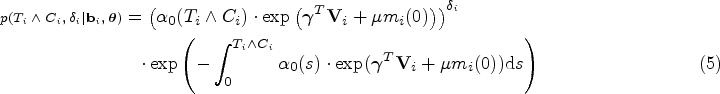
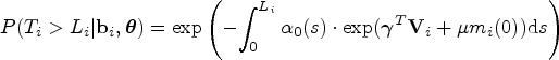
We suggest a Cox proportional hazards model for the individual event hazard of the form

Following Bayesian joint models, we assume a penalized B-spline to approximate the logarithm of the baseline hazard

As explained earlier and investigated in more depth in the remainder of the paper, the novelty of the application of model (1) and model (2) is that the combination of both models is not used to estimate the effect of the time-dependent value
Let
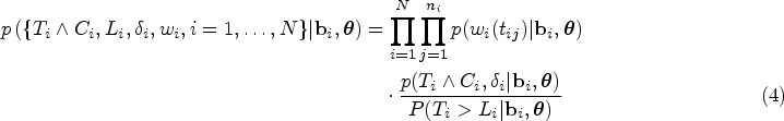
Following the Bayesian framework of Piulachs et al.,
26
the overall joint likelihood conditioned on the random effects


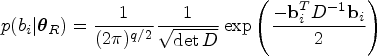
In the following, we use standard priors to fit the models of the Bayesian approach.23,26,31 In particular, normal priors are taken for the parameter of the fixed effects
Software to fit these joint models with left truncation is readily available in the
The following simulation study investigates the performance of our proposed approach under left-truncated scenarios. The scenarios are motivated by the study example and are chosen such that they differ in the percentage of left truncation, sample size, number of follow-up visits, and direction of the association between the longitudinal and the survival submodel. The
Simulation scenarios: For each scenario, 1000 datasets are generated.
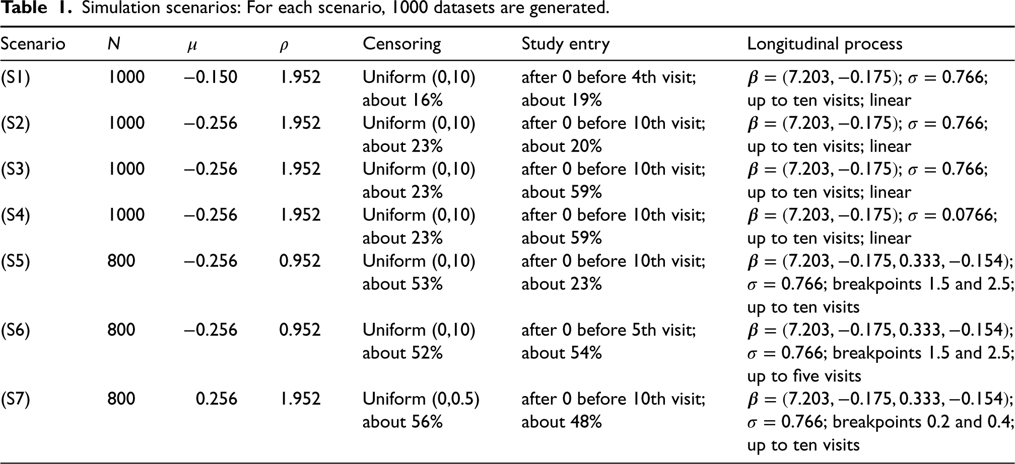
Simulation scenarios: For each scenario, 1000 datasets are generated.
The survival time
Scenarios (S1), (S2), (S3), and (S4) assume the linear longitudinal trajectory to be given by


Scenario (S1) is rather simple. With an HR based on the association parameter of
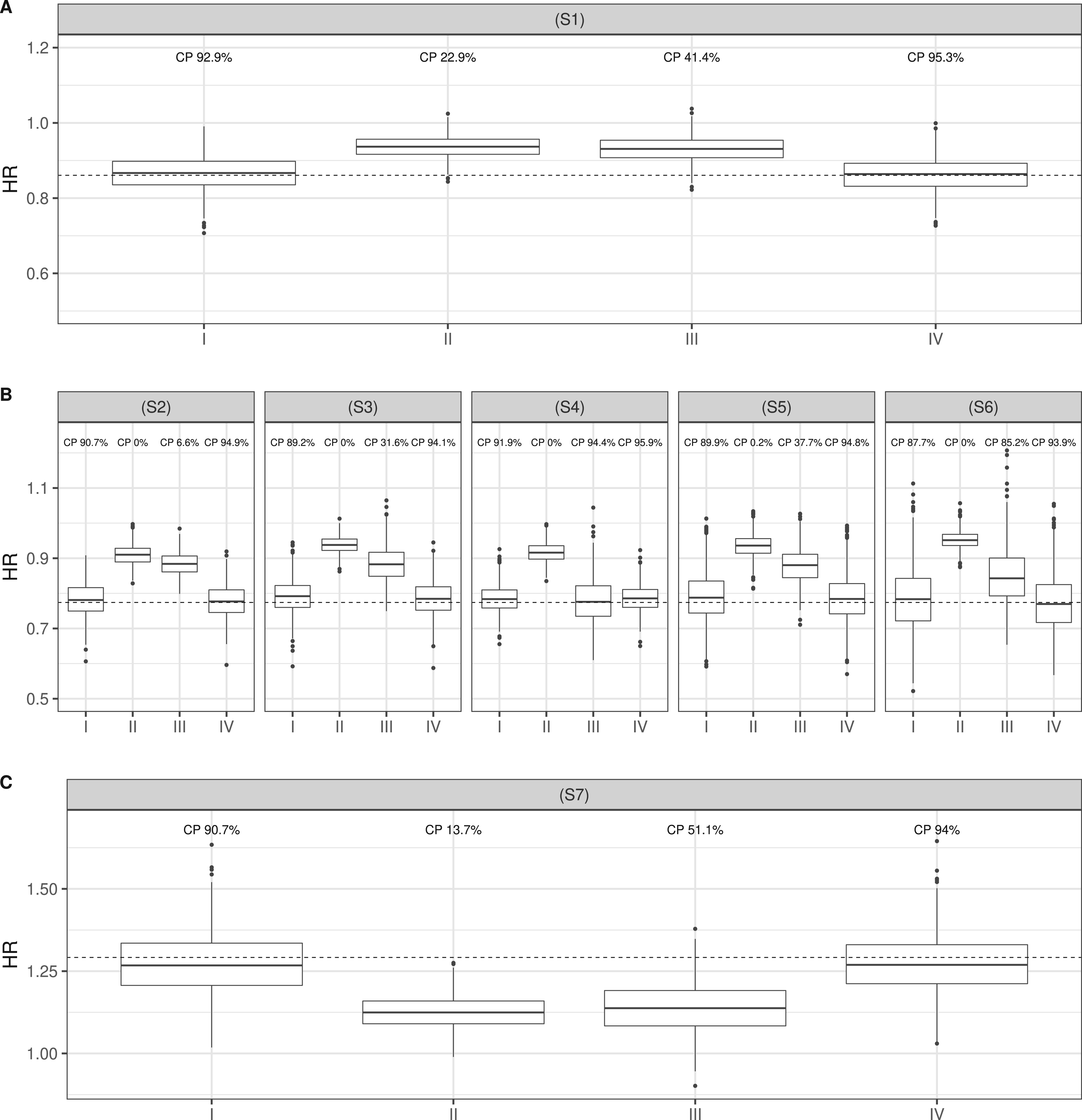
We simulate 1000 datasets of each scenario and set the confidence level to 95%. To each simulated dataset, we apply our proposed model (I) and a standard Cox proportional hazards model incorporating the observed covariate value of the time-dependent longitudinal covariate at study entry (II). The latter would model the individual event hazard as

Furthermore, we consider two alternative approaches, a complete case analysis using only the observations entering at the time origin 0 (III), and a two-stage approach, first fitting a linear mixed-effects model and predicting the baseline value of the covariate for all individuals, and then inserting the prediction into the Cox proportional hazards model (IV). The rationale behind approach III is that we have assumed left truncation to be independent of the times-to-event. The motivation behind approach IV is that it will be easier to fit.
The results of the association parameter
Simulation results regarding the association parameter
Our proposed model provides negligible bias and coverage probabilities (CPs) close to 90%. Compared to scenarios (S1) and (S2), the joint model approach performed slightly worse in scenarios (S3) and (S4) (relative bias of
The complete case analysis is also heavily biased in all scenarios except (S4), where the standard deviation of the error terms is very small (relative bias between
Simulation results regarding the association parameter
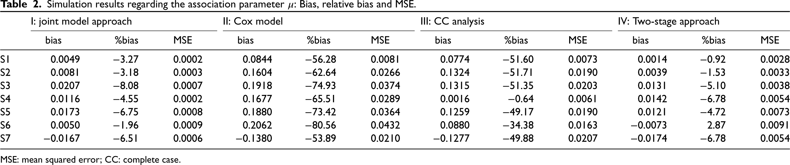
MSE: mean squared error; CC: complete case.
The data example is from a population-based study of patients diagnosed with type 2 diabetes and under first-line OAD medication. 1 One aim was to access the association of prognostic baseline factors on the time to treatment failure. Thereby, treatment failure was defined as either the initiation of basal-supported oral therapy (BOT) or stopping first-line OAD, whatever comes first. The data source was the DIVE register, which is a German prospective, observational, multicenter diabetes register established in 2011. 2 Since the natural timescale of the analysis is “time since start of first OAD medication”, but data collection occurs in calendar time and with start of the DIVE register, the data are subject to left truncation (see Figure 1). The original study fitted a Cox proportional hazards model accounting for left truncation and incorporating longitudinal covariate values measured at study entry. However, it has been discussed that statements regarding baseline effects are questionable due to unmeasured baseline information for left-truncated individuals.1,7
The proposed methodology extends these previous results by utilizing the entire available longitudinal information to estimate baseline effects at OAD initiation. The present study cohort focuses on the 16,719 individuals, which have at least two observed longitudinal HbA1c measurements during follow-up and censors at year 20. The reasons are that neither only one observed HbA1c measurement per individual nor sparse measurements after year 20 are sufficient in order to adequately fit a linear mixed-effects model according to relation (1). A total of 69,363 longitudinal measurements were taken in this study cohort. In total, we observed 2023 patients initiating BOT and 5004 ones stopping OAD. About 62% of all patients entered the study cohort with delay.
The fitted univariate Cox model shows a 8.8% increased hazard risk for treatment failure for each unit increase in the HbA1c level at study entry (HR: 1.088, 95% confidence interval: [1.070, 1.106]). This is comparable to the result provided by the original study cohort (HR: 1.084, 95% confidence interval: [1.068, 1.102]) and in line with clinical expertise that higher HbA1c levels are conjoined with a higher risk of antidiabetic treatment failure. 35
Now, moving to our proposed joint modeling framework, we assume a piecewise linear mixed-effects model with breakpoints at 2.5 and 4.5 years for the HbA1c trajectory:

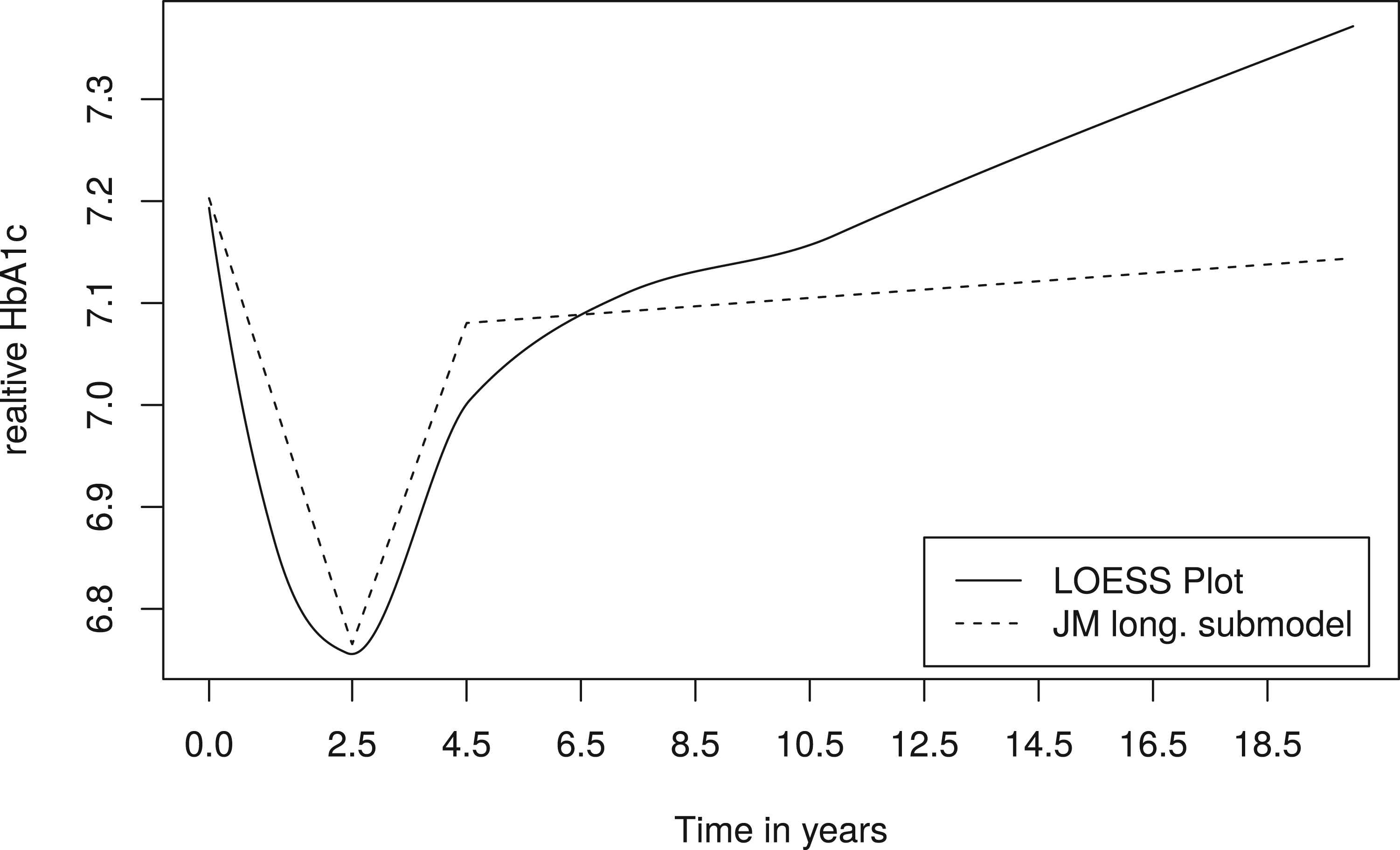
LOESS plot of the HbA1c trajectory (straight line) and trajectory obtained from estimated coefficients of the longitudinal (long.) submodel (dashed line). LOESS: locally estimated scatterplot smoothing; HbA1c: haemoglobin A1c; JM: Joint Model.
In contrast to the original Cox analysis, the joint model results in a more pronounced effect (HR: 1.292, 95% credible interval: [1.254, 1.337]). The effect estimated by the complete case analysis is similar to the original Cox analysis (HR: 1.074, 95% confidence interval: [1.047, 1.102]). The two-stage approach shows a more pronounced effect that is also more pronounced than that of the joint model (HR: 1.405, 95% confidence interval: [1.366, 1.445]). One possible explanation of the smaller effect seen in the standard Cox analysis is that patients with delayed study entry have an HbA1c value upon study entry that is already regulated by medication, attenuating association. However, the fact that the complete case analysis found an effect more in line with standard Cox rather than joint modeling or two-stage suggests a second possible explanation, namely the presence of measurement error.
Additionally, we also considered the estimated longitudinal trajectory (see Figure 3, dashed line), with estimated fixed effects
As sensitivity analyses (not shown), we also considered earlier breakpoints based on the literature and added another breakpoint at 10.5, but the results of the association parameter and the estimated intercept
In this analysis, we have interpreted time-to-event
We have proposed an innovative use of the joint model framework to suggest a solution to a longstanding problem in observational studies with delayed entry: the estimation of baseline effects of longitudinal covariates associated with time-to-event outcomes in the presence of unmeasured baseline information due to delayed study entry. Our approach takes advantage of established joint modeling techniques, but considering baseline effects of the longitudinal trajectory in combination with delayed study entry is beyond the standard applications of joint models. In contrast, standard joint modeling targets missing longitudinal covariate information for right-censored time-to-event data. The simulation found a satisfactory performance of our method under different specifications of left truncation and the longitudinal trajectory. In contrast, the often used Cox model accounting for left truncation but incorporating the respective measurement at study entry rather than at baseline leads to biased results when the interest is in the baseline effect. This has been discussed in the literature 6 and was supported by the present simulation study. Even though, at first, one would expect the complete case analysis to be unbiased provided that delayed study entry is entirely unrelated to the time-to-event process of interest, we found that the complete case analysis may also be biased in the presence of measurement error. These findings are in line with Crowther et al., 13 who, however, considered a non-left-truncated setting such that baseline covariates are known and measurement error was at the core of the investigation. Parts of the bias of the Cox model incorporating the study entry measurements might, therefore, also be attributed to ignoring measurement error. Furthermore, we found a two-stage approach, first predicting the baseline values of the covariate and then including the predictions into the Cox proportional hazards model, to be another alternative to deal with the problem. We found the two-stage approach to be unbiased in the simulations, one reason arguably being that a Cox model with baseline covariates only does not include the longitudinal trajectory modeled in the first stage. The theoretical disadvantage of this “naive” two-stage approach is that, unlike joint modeling, the variability in the prediction in the first stage is not included in the second stage. 34 Furthermore, in scenarios with a stronger correlation between the longitudinal and the survival process, the joint modeling approach might be preferable to the two-stage approach. 18 We illustrated the procedures with register-based diabetes data and found that higher HbA1c levels at baseline are associated with an increased risk of treatment failure. This result supports the findings of the original study, but both joint model and two-stage analyses found more pronounced effects than a Cox regression of study entry values and a complete case analysis. Possible reasons are both the fact that HbA1c values at later study entry are already medically regulated and also possible measurement error. However, using a Cox regression would also lead to a biased estimated association, even if all baseline HbA1c measurements were known, as the measurement error is neglected during estimation.
We used Bayesian joint models as the joint models accounting for left truncation and lagged effects were readily implemented in the
The proposed methodology is not restricted to register-based diabetes trials but has potential in other fields of epidemiological research. Typical examples include aging studies, 35 fracture studies in health services research, 36 or infection control trials in healthcare epidemiology. 37 However, in studies in which all individuals are left-truncated, for example, in pregnancy outcome studies, 38 the proposed method has restrictions. Having a subset of patients with measurements at the time origin will be most useful for estimation of the longitudinal trajectory. Furthermore, under heavier left truncation and sparse information about the longitudinal covariate, the joint model approach was found to have increased relative bias, although it still performed better than the standard Cox approach (simulation scenario (S5)).
In the analysis of the DIVE data, we have already discussed the need to account for competing risks. If mortality information had been available, one option would have been a composite endpoint of OAD failure or death, whatever came first. Alternatively, a joint model for competing risks may be investigated.12,15,31,39 For the DIVE data, a finer competing risks investigation would consider endpoints “BOT initiation” and “OAD refusal prior to BOT”.1,7 Finally, the question of a “baseline” effect is not necessarily restricted to the original time zero, but may also be investigated at a later time point
Supplemental Material
sj-zip-1-smm-10.1177_09622802231163334 - Supplemental material for Modeling unmeasured baseline information in observational time-to-event data subject to delayed study entry
Supplemental material, sj-zip-1-smm-10.1177_09622802231163334 for Modeling unmeasured baseline information in observational time-to-event data subject to delayed study entry by Regina Stegherr, Jan Beyersmann, Peter Bramlage and Tobias Bluhmki in Statistical Methods in Medical Research
Footnotes
Acknowledgements
The authors thank an anonymous reviewer of this article, whose valuable suggestions greatly contributed to the improvement of the manuscript.
Declaration of conflicting interests
The authors declared no potential conflicts of interest with respect to the research, authorship, and/or publication of this article.
Funding
The authors disclosed receipt of the following financial support for the research, authorship, and/or publication of this article: RS and TB were partially supported by Grant [BE 4500/3-1] of the German Research Foundation (DFG).
Supplemental material
Supplemental material is available for this article online.
References
Supplementary Material
Please find the following supplemental material available below.
For Open Access articles published under a Creative Commons License, all supplemental material carries the same license as the article it is associated with.
For non-Open Access articles published, all supplemental material carries a non-exclusive license, and permission requests for re-use of supplemental material or any part of supplemental material shall be sent directly to the copyright owner as specified in the copyright notice associated with the article.