Causal simulation experiments: Lessons from bias amplification

Abstract

Recent theoretical work in causal inference has explored an important class of variables which, when conditioned on, may further amplify existing unmeasured confounding bias (bias amplification). Despite this theoretical work, existing simulations of bias amplification in clinical settings have suggested bias amplification may not be as important in many practical cases as suggested in the theoretical literature. We resolve this tension by using tools from the semi-parametric regression literature leading to a general characterization in terms of the geometry of OLS estimators which allows us to extend current results to a larger class of DAGs, functional forms, and distributional assumptions. We further use these results to understand the limitations of current simulation approaches and to propose a new framework for performing causal simulation experiments to compare estimators. We then evaluate the challenges and benefits of extending this simulation approach to the context of a real clinical data set with a binary treatment, laying the groundwork for a principled approach to sensitivity analysis for bias amplification in the presence of unmeasured confounding.

1 Introduction

Causal identification strategies aim to condition on a sufficient set of observables such that the potential outcomes are conditionally independent of the treatment of interest.^1–3 Causal variable selection procedures often assume that at least one subset of the observed variables forms such a sufficient set. ⁴ The object in causal variable selection then becomes how to separate variables which are necessary for identification of the causal effect from those variables which are extraneous^4,5 in the interest of reducing estimator variance or covariate dimensionality.^4,6

In non-experimental observational studies, we do not have full access to a sufficient set in many realistic settings, and important confounding pathways remain unblocked.^7,8 This is referred to as unmeasured confounding or endogeneity in the statistics and econometrics literatures, respectively. However, applied researchers currently rely on variable selection techniques such as lasso, step-wise, change-in-estimator selection, and outcome and/or treatment oriented approaches ⁹ despite violating their underlying assumptions.

Often, variable selection techniques are used to avoid conditioning on negligible confounding pathways without introducing meaningful bias to the estimator. In this paper, we explore how this intuition can break down under even mild violations of the underlying assumptions. In particular, we build on the work of Pearl ¹⁰ and explore how treatment prediction-oriented approaches may inadvertently amplify bias if unmeasured confounding pathways remain. We use the lessons from this failure of intuition to better understand the consequences of variable selection in both linear models and partially linear orthogonalized models in the presence of important unmeasured confounding. We then build a principled approach to simulate from such systems of equations which may be used to compare the theoretical properties of different estimators, such as accurately quantifying the change in bias when we modify the causal relationship between a confounder and the treatment, or for the purpose of sensitivity analysis.

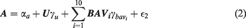
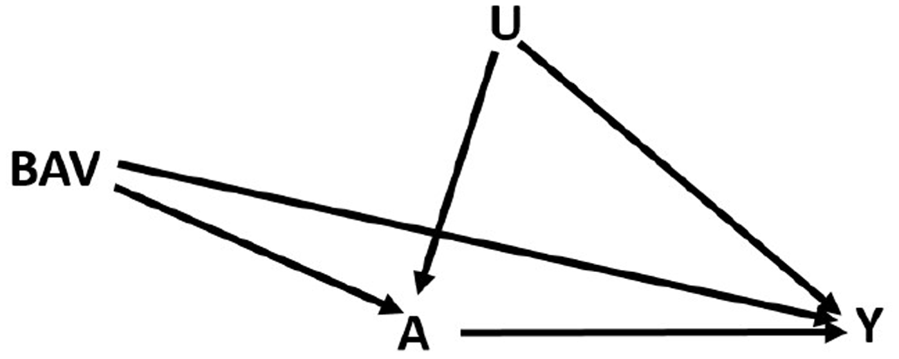
First consider data generated from the following directed acyclic graph (DAG) (Figure 1) and set of structural equations

$$\mathit{Y}={\alpha }_y+\mathit{A}{\beta }_a+\mathit{U}{\beta }_u+{ϵ}_1$$

(1)

$$\mathit{A}={\alpha }_a+\mathit{U}{\gamma }_u+{\displaystyle \sum _{i=1}^{10}\mathit{BA}{\mathit{V}}_{\mathit{i}}}{\gamma }_{ba{v}_i}+{ϵ}_2$$

(2)

$$\mathit{U}={\alpha }_u+{\displaystyle \sum _{i=1}^{10}\mathit{BA}{\mathit{V}}_{\mathit{i}}}{\psi }_{ba{v}_i}+{ϵ}_3$$

(3)

Figure 1.

Directed acyclic graph (DAG): Meyers (2011) extended to 10 possible bias amplifying variables BAVs.

where Y is the outcome, A is the treatment of interest, U is an unmeasured variable, BAV refers to 10 different potential bias amplifying variables that are measured and affect both A and U but have no direct effect on Y , γ_x is the coefficient for the effect of the variable on A , β_x is the coefficient for the effect of the variable on Y , and ϵ_number is an error term for the corresponding equation. This model contains one confounding path that cannot be blocked ( $\mathit{A}\leftarrow \mathit{U}\to \mathit{Y}$ ) and 10 confounding paths ( $\mathit{A}\leftarrow \mathit{BA}{\mathit{V}}_{\mathit{1}}\to \mathit{U}\to \mathit{Y}$ ; …; $\mathit{A}\leftarrow \mathit{BA}{\mathit{V}}_{\mathit{10}}\to \mathit{U}\to \mathit{Y}$ ) that can be blocked by including the measured $\mathit{BA}{\mathit{V}}_{\mathit{i}}$ variables in the model. However, including any of these $\mathit{BA}{\mathit{V}}_{\mathit{i}}$ might also increase bias (potential bias amplifying variables). Our goal is to find the least biased estimator of the average causal effect (ACE) of treatment (β_a).

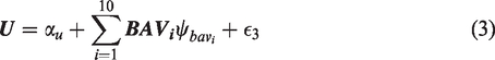
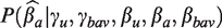
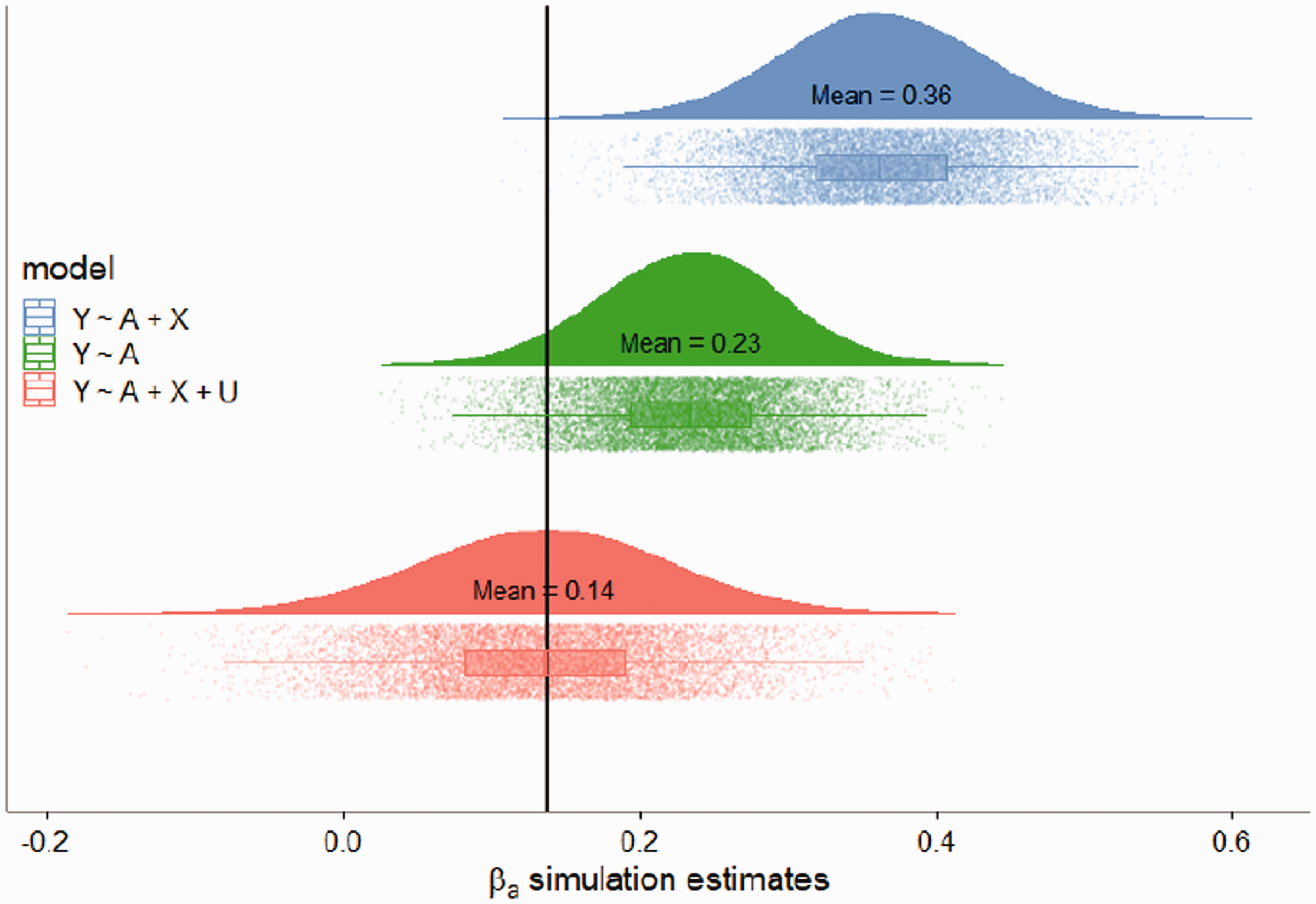
By including more of the BAV variables in the model, intuition suggests the remaining unmeasured confounding bias should decrease because more potential confounders have been included in the conditioning set. However, as demonstrated in the bias amplification literature,^10–12 conditioning on confounders may still increase bias. For example, suppose further the 10 observable variables account for 90% of the variance in the variable U responsible for unmeasured confounding. The blue violin plot in Figure 2 represents the sampling distribution of the estimator from the true outcome model that includes the treatment and both measured/unmeasured confounding variables included as regressors. As expected, the estimates are approximately normally distributed around the true value ${\beta }_a=0.7$ . The green violin plot represents the biased estimates from the naive model, the simple regression of the outcome Y on the treatment A , which does not include any of the confounders (measured or unmeasured). The red violin plot represents the linear model adjusted for all 10 measured confounders which account for 90% of the unmeasured confounding. The adjusted model performs much worse than the naive model both in terms of bias (0.73 compared to 0.43, interpretable as standard deviations) and variance (standard deviation of 0.1 compared to 0.02). In fact, in 4990 of 5000 simulations the adjusted estimate was farther from the truth than the naive estimate and nearly 65% of the adjusted estimates had the incorrect effect sign.

Figure 2.

Violin plot from simulations from equations (1) to (3). There were 5000 replication with n = 5000. The true effect of interest was ${\beta }_a=0.7$ , represented by the blue line. The confounding effects were ${\beta }_u=-0.5$ and ${\gamma }_u=0.59$ . The vector of coefficients for BAV on U was ${\psi }_{\mathit{bav}}=\{-0.55,-0.45,-0.3,0.30,.25,0.20,-0.20,0.20,-0.15,0.10\}$ , which in general were larger than the impact of BAV on A , ${\gamma }_{\mathit{bav}}=\{-.1,-.15,-.1,.21,-.2,.3,-.2,-.15,-.2,.075\}$ . $\mathit{U},\mathit{BAV},\mathit{A},$ and Y are all standard normal variables. The error terms were normally distributed with standard deviations: ${\sigma }_1=0.93,{\sigma }_2=0.07$ , and ${\sigma }_3=0.32$ . All intercepts were set to 0. The code to reproduce the plot can be found in the supplementary materials. The red vertical line represents $\widehat{{\beta }_a}=0$ .

The purpose of this paper is to explain why model selection intuition fails us in this case and how we can use a combination of data and simulation approaches to improve model selection. We build upon an emerging theoretical literature exploring a class of variables which can amplify existing unmeasured confounding bias,^{10,13,14,30,31,32,35} called bias amplifiers. Throughout this text, we will refer to (potential) bias amplifiers as those variables which, upon their inclusion in a model, (may) increase the absolute bias in the estimation of particular target parameters relative to a smaller, nested model. In the above example, all 10 BAV s increase the bias due to the path $\mathit{A}\leftarrow \mathit{U}\to \mathit{Y}$ and in fact could also increase the bias of any other variable BAV if it were not included in the model, since they are all confounders.

The class of bias-amplifying variables is potentially very large and common in practical applications. Bias amplification occurs when the absolute bias of an estimator for a target parameter is larger than the absolute bias of an estimator for a competing, nested model. In this text, we define the natural model comparison to be the naive regression of the outcome ( Y ) on the treatment ( A ) and bias amplification will be the additional relative bias that results from adding additional predictors. Throughout, the goal of model selection in this context will be to choose the variables and thus the model which minimizes bias in estimating the true average treatment of effect in the presence of unmeasured confounding pathways.

We adopt a matrix notation framework to characterize this problem because (1) we can more easily generalize to a much larger class of directed acyclic graphs and structural equations than previously studied; (2) it offers a unifying geometric explanation for the amplified bias in the context of least squares estimation; and (3) it offers a solid foundation for how to build data-informed model selection procedures. Finally, we develop a procedure for simulating from a more complete parameter space in a way that respects the underlying amplification process. In addition to lending itself better to articulating and answering causal simulation questions, this procedure helps explain why some previous studies have incorrectly concluded that applied investigators need not worry about amplification in practice. ¹⁵ We evaluate the challenges of implementing this approach with a real clinical example with binary treatment.

2 Problem formulation

Figure 3 shows a basic directed acyclic graph (DAG) which has both measured and unmeasured confounding. Let Y represent the outcome and let A be the treatment or variable of interest. Let U be an unmeasured confounding variable that we cannot include in a regression model, but which has a functional relationship with both Y and A . The bias amplifying variable ( BAV ) in this DAG is analogous to U in that it is a cause of Y and a cause of A ; however, we are able to measure BAV and not U . Intuition from currently recommended causal variable selection techniques would tell us to include BAV in the regression to reduce bias because it is the root of a confounding path ( $\mathit{A}\leftarrow \mathit{BAV}\to \mathit{Y}$ ). However, as has been demonstrated,^10–12,14 blocking this confounding path can actually increase or amplify the bias relative to the naive estimator that depends only on A .

Figure 3.

DAG: Two confounding paths, where A is the treatment of interest, Y is the outcome, U is an unmeasured variable and BAV is a measured variable.

Assume that we now restrict the possible models for the DAG in Figure 3 to only linear associations amongst variables. The data generating model (or causal structural equations) representing Figure 3 under strictly linear association can be written as

$$\mathit{Y}={\alpha }_y+\mathit{A}{\beta }_a+\mathit{U}{\beta }_u+\mathit{BAV}{\mathit{\beta }}_{\mathit{bav}}+{ϵ}_{\mathit{1}}$$

(4)

$$\mathit{A}={\alpha }_a+\mathit{U}{\gamma }_u+\mathit{BAV}{\mathit{\gamma }}_{\mathit{bav}}+{ϵ}_{\mathit{2}}$$

(5)

where α_y and α_a are the intercept terms for Y and A , respectively. As noted above, we use the form β_x throughout this paper to denote true structural coefficients for some variable X on the outcome Y . For example, the true structural coefficient for U on Y is β_u. Analogously, the true regression parameter for some variable X on the treatment A is represented by γ_x. The estimates of these parameters by OLS are denoted by $\widehat{{\beta }_x},\widehat{{\gamma }_x}$ with additional superscripts to clarify which set of estimating equations the estimator is derived from. By assumption ${ϵ}_{\mathit{1}}$ and ${ϵ}_{\mathit{2}}$ are error terms independent of each other we further assume that $E[{ϵ}_{\mathit{1}}|\mathit{A},\mathit{U},\mathit{BAV}]=0$ and $E[{ϵ}_{\mathit{2}}|\mathit{A},\mathit{BAV}]=0$ , and that the error terms have some finite variance ${\sigma }_{{ϵ}_{1,2}}^2$ . In simulation experiments, we typically simulate from normal distributions which are independent from all other variables, but only the above assumptions are necessary for the theoretical results to hold.

We also assume that the target estimand is the ACE. In the linear model case, this is simply the β_a above in equation (4) (See Appendix A.3.I for derivation of the ACE). U is unmeasured and thus we cannot identify the ACE from the observed data if ${\beta }_u\ne 0$ , but we are interested in estimating the quantity with as little bias as possible.

2.1 Matrix notation and probability limits

To tackle the question of model selection, we must derive properties of different $\widehat{{\beta }_a}$ estimators, with the restriction that the estimators be functions of only observed variables, under different assumed conditional regression models. To this aim, we propose expressing OLS estimates using matrix notation and ideas borrowed from the partial regression literature. Further, we propose considering also the probability limits of the estimators to extend our results to more general and realistic cases of bias amplification (see Appendix A.2). For the naive estimator, we use a simple linear regression to estimate a conditional expectation of the form

$$E[\mathit{Y}|\mathit{A}]={\alpha }_y^{\mathit{naive}}+\mathit{A}{\beta }_a^{\mathit{naive}}+{\mathit{\upsilon }}_{\mathit{1}}$$

(6)

where ${\mathit{\upsilon }}_{\mathit{1}}$ is the error of the regression term. Unbiased estimation of the naive model by OLS, and thus of the true conditional expectation $E[\mathit{Y}|\mathit{A}]$ , requires the assumption that $E[{\mathit{\upsilon }}_{\mathit{1}}|\mathit{A}]=0$ . However, this of course is not true since according to the data generating equation (4), the error will be a function of the confounding terms, resulting in non-zero bias. The naive estimator bias is a special case of the classic omitted variables problem, where we have two omitted variables which are related to both the treatment and the exposure, U and BAV .

Let ${\widehat{{\beta }_a}}^{\mathit{naive}}$ be the estimate of β_a from the naive model (6). Throughout this paper, we will consider the matrix Z to be a matrix of all the variables that we include in a regression that are not the variable of interest A , in other words control variables in a selection on observables approach. In the naive model, $\mathit{Z}=\mathit{1}$ where throughout 1 will denote an $n\times 1$ vector of 1 s. In matrix notation, applying the Frisch-Waugh-Lovell (FWL) theorem (see Appendix A.1), we can write ${\widehat{{\beta }_a}}^{\mathit{naive}}$ as

$${\widehat{{\beta }_a}}^{\mathit{naive}}=\frac{{\mathit{A}}^{\mathit{T}}{\mathit{M}}_{\mathit{1}}\mathit{Y}}{{\mathit{A}}^{\mathit{T}}{\mathit{M}}_{\mathit{1}}\mathit{A}}$$

(7)

where ${\mathit{M}}_{\mathit{1}}$ is a centering projection matrix, defined and described in detail in Appendix section A.1. In the case of linear relationships between all the variables, following Pearl, ¹⁰ this estimator has the following expectation

$$E[{\widehat{{\beta }_a}}^{\mathit{naive}}]={\beta }_a+({\beta }_u{\gamma }_u{\sigma }_u^2+{\beta }_{\mathit{bav}}{\gamma }_{\mathit{bav}}{\sigma }_{\mathit{bav}}^2)\frac{1}{{\sigma }_a^2}$$

(8)

The absolute bias for the ACE then clearly is $|({\beta }_u{\gamma }_u{\sigma }_u^2+{\beta }_{\mathit{bav}}{\gamma }_{\mathit{bav}}{\sigma }_{\mathit{bav}}^2)\frac{1}{{\sigma }_a^2}|$ . Now consider the estimates resulting from further conditioning on the observable BAV variable, i.e. estimating a conditional expectation of the form

$$E[\mathit{Y}|\mathit{A},\mathit{BAV}]={\alpha }_y^{\mathit{naive}}+\mathit{A}{\beta }_a^{\mathit{bav}}+\mathit{BAV}{\beta }_{\mathit{bav}}^{\mathit{bav}}+{\mathit{\upsilon }}_{\mathit{2}}$$

(9)

We will denote the resulting estimator ${\widehat{\beta }}_a^{\mathit{bav}}$ which can be written as follows by again applying the FWL theorem

$${\widehat{\beta }}_a^{\mathit{bav}}=\frac{{\mathit{A}}^{\mathit{T}}{\mathit{M}}_{\mathit{z}}\mathit{Y}}{{\mathit{A}}^{\mathit{T}}{\mathit{M}}_{\mathit{z}}\mathit{A}}$$

(10)

where $\mathit{Z}=[\mathit{1},\mathit{BAV}]$ and ${\mathit{M}}_{\mathit{z}}$ is the annihilator projection matrix of the matrix Z (see Appendix A.1 for details and properties). Again following Pearl, ¹⁰ the expectation of $\widehat{{\beta }_a^{\mathit{bav}}}$ is

$$E[\widehat{{\beta }_a^{\mathit{bav}}}]={\beta }_a+({\beta }_u{\gamma }_u{\sigma }_u^2)\frac{1}{{\sigma }_a^2-{\gamma }_{\mathit{bav}}^2{\sigma }_{\mathit{bav}}^2}$$

(11)

In Appendix A.4, we explicitly show Pearl’s derivation and how it relies on the conditional expectation $E[\mathit{U}|\mathit{A},\mathit{BAV}]$ being linear in both A and BAV . Pearl’s derivation is limited in that it is cumbersome and does not generalize well to a broad class of DAGs and functional forms. A simple example where we are unable to use Pearl’s method is the case of an interaction term in the exposure structural equation between U and BAV . This implies that $E[\mathit{U}|\mathit{A},\mathit{BAV}]$ is nonlinear in A and BAV . This cannot be represented by an unbiased least squares projection of the form $\mathit{U}={\alpha }_u+\mathit{A}{\zeta }_a+\mathit{BAV}{\zeta }_{\mathit{bav}}+{ϵ}_{\mathit{3}}$ as required by Pearl’s derivation method (see Appendix A.4 for details), where ζ_i represents the true regression coefficient for variable i. If we impose further strict distributional assumptions over all the variables, we may still be able to directly solve the conditional expectation and find an expression for bias in terms of the underlying parameters. However, in many applied cases, these distributional assumptions will not be justified, particularly assuming a distribution for the unmeasured confounding which will always be untestable.

In contrast, if we consider the probability limits, we do not need to assume that $E[\mathit{U}|\mathit{A},\mathit{BAV}]$ is linear, nor do we have to make any additional distributional assumptions to find meaningful limiting expressions for our estimators in a broad class of clinically relevant circumstances. In addition to giving rise to a meaningful interpretation, the closed form asymptotics we derive allow us to more easily harness domain knowledge about the underlying causal process for the purpose of model selection.

Since we are still interested in the finite sample expectation of the estimators and the bias directly, we report the expectations when appropriate and feasible. The probability limit facilitates insight under weaker assumptions than those necessary to derive exact forms of the expectations. Additionally, in some cases, like the linear model of Pearl, ¹⁰ the probability limits for ${\widehat{\beta }}_a^{\mathit{naive}}$ and ${\widehat{\beta }}_a^{\mathit{bav}}$ are precisely equal to their expectations (see Appendix A.7).

3 Treatment variance explained and amplifying effects for strictly linear models

In this section we examine the probability limits of the estimators to better understand the mechanics and root causes of bias amplification. First, notice the denominator of equation (11) ( ${\sigma }_a^2-{\gamma }_{\mathit{bav}}^2{\sigma }_{\mathit{bav}}^2$ ) gets smaller as the causal edge $\mathit{BAV}\to \mathit{A}$ increases in strength. This is because when we specify the functional form of a system of random variables and conditional independence assumptions, we are also determining a formula for its variance. Under the structural equation we specified for the exposure (equation (5), with the corresponding DAG shown later in Figure 7(a)), ${\sigma }_a^2-{\gamma }_{\mathit{bav}}^2{\sigma }_{\mathit{bav}}^2$ is precisely equal to the remaining residual treatment variance in A after having adjusted for BAV in a regression model. When we assume that all the variables are standardized, this term becomes $1-{\gamma }_{\mathit{bav}}^2$ as presented in Pearl ¹⁰ (under the assumption of standard normal, here we drop the distributional requirement), because the variance of standard normal variables is equal to 1 ( ${\sigma }_a^2,{\sigma }_{\mathit{bav}}^2=1$ ).

In order to visualize this phenomenon, we use ideas from partial regression plots. ¹⁶ By the FWL theorem, we can always pre-multiply an estimating equation by the residual-making variables of a set of regressors and get the same estimates (see Appendix A.1 for further details). For example, the following two regression equations produce the same numerical ordinary least squares estimates of ${\widehat{{\beta }_a}}^{\mathit{naive}}$

$$\mathit{Y}={\alpha }_y+\mathit{A}{\beta }_a+{\mathit{\upsilon }}_{\mathit{1}}$$

(12)

$${\mathit{M}}_{\mathit{1}}\mathit{Y}={\mathit{M}}_{\mathit{1}}\mathit{A}{\beta }_a+{\mathit{\upsilon }}_{\mathit{1}}$$

(13)

Equation (13) is the model for a simple linear regression of a modified outcome, ${\mathit{M}}_{\mathit{1}}\mathit{Y}$ , on a modified treatment, ${\mathit{M}}_{\mathit{1}}\mathit{A}$ (see Appendix A.1). There is no intercept term as the mean of the modified treatment must be equal to zero.

$$\mathit{Y}={\alpha }_y+\mathit{A}{\beta }_a+\mathit{BAV}{\beta }_{\mathit{bav}}+{\mathit{\upsilon }}_{\mathit{2}}$$

(14)

$${\mathit{M}}_{\mathit{z}}\mathit{Y}={\mathit{M}}_{\mathit{z}}\mathit{A}{\beta }_a+{\mathit{\upsilon }}_{\mathit{2}}$$

(15)

Similarly equations (14) and (15) above produce equivalent ordinary least squares estimates of ${\widehat{\beta }}_a$ , where $\mathit{Z}=[\mathit{1}\mathit{BAV}]$ is a column of 1 s and the BAV variable. Equation (15) is a single variable regression on a transformed set of variables. The modified Y is produced by taking the residuals from regressing Y on a column of 1 s and BAV . In other words, the dependent variable is the residual vector resulting from regressing Y on an intercept column and BAV . The independent variable is the residual vector resulting from regressing A on a column of 1 s and BAV . Another way to think of the residuals is in the context of orthogonalization techniques, where ${\mathit{A}}^{\mathit{T}}{\mathit{M}}_{\mathit{z}}$ for example is the part of A orthogonal to linear combinations of the control variables A . We then regress the orthogonalized outcome on the orthogonalized treatment, which is implicitly the mechanics of what happens whenever we use least squares estimation. See section 4.2 for more general orthogonalization techniques.

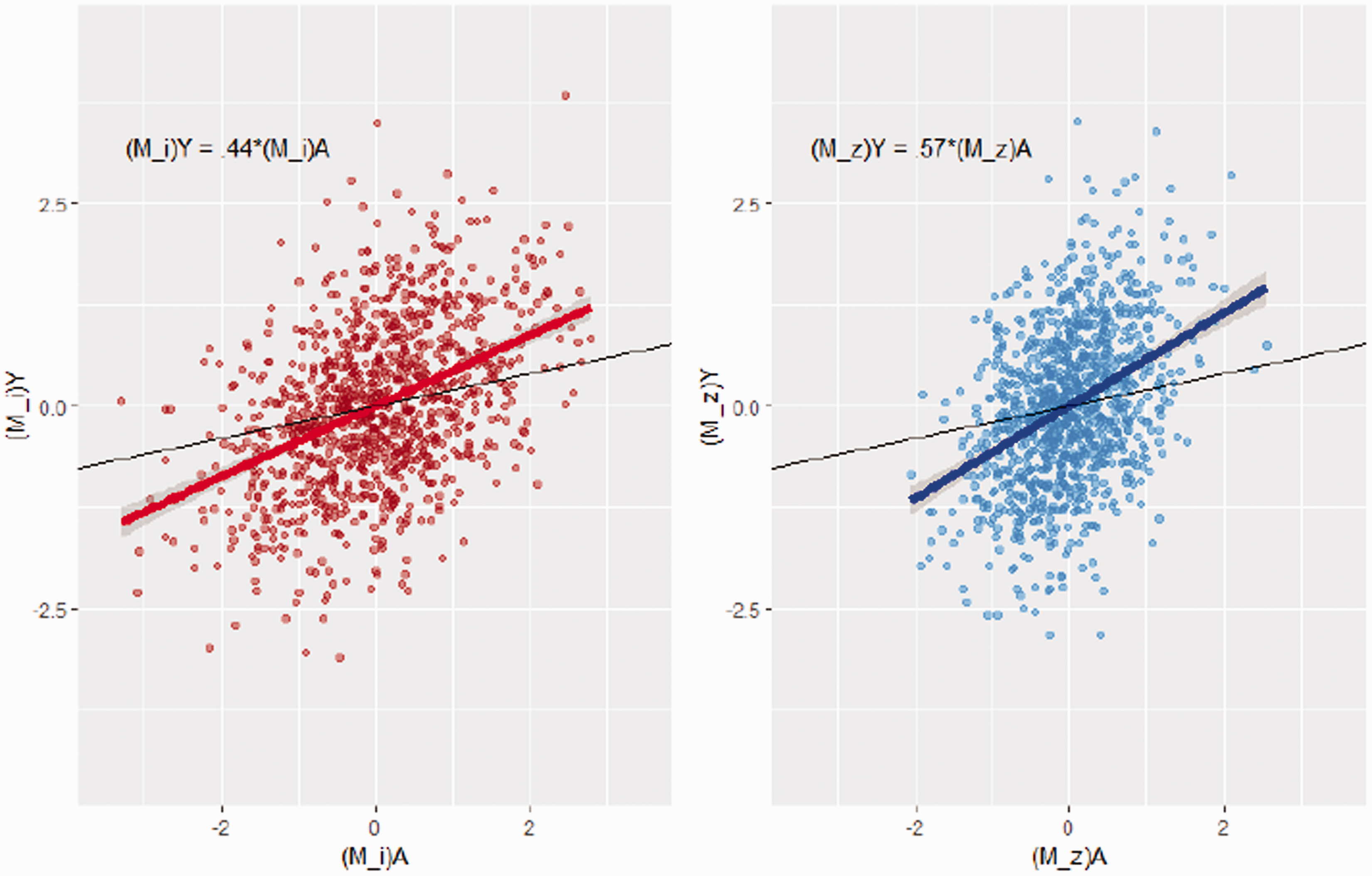
Since we have reduced the multi-variable regression problem to a simple linear regression for two linearly transformed variables, we can easily visualize the amplification process via a partial regression plot. In Figure 4 the left subplot visualizes the naive regression equation (13), whereas the blue subplot on the right visualizes the regression equation (15) that includes BAV . The data were simulated from a special case of equations (4) and (5), with n = 1000. Details can be found in the appendix (Appendix section A.13).

Figure 4.

In both panels, the unbiased ACE ( ${\beta }_a=0.2$ ) is shown by the dotted black line. In the left panel, the red dots represent the centered treatment ( ${\mathit{M}}_{\mathit{\iota }}\mathit{A}$ ) plotted against the centered outcome ( ${\mathit{M}}_{\mathit{\iota }}\mathit{Y}$ ) and the estimated slope ${\widehat{\beta }}_a^{\mathit{naive}}$ is shown with the bolded red line. This represents the equivalent regressions in equations (12) and (13). In the right panel, the blue dots represent the modified treatment ( ${\mathit{M}}_{\mathit{z}}\mathit{A}$ ) plotted against the modified outcome ( ${\mathit{M}}_{\mathit{z}}\mathit{Y}$ ). The solid blue line represents the treatment estimate from the equivalent regressions (14) and (15).

The unbiased ACE is the slope of the black line ( ${\beta }_a=0.2$ ) in these plots. The slope of the blue line (equal to the OLS estimator from the amplifying model) is clearly farther away from the true slope (in black) compared to the slope of the red line from the naive model, and thus the conditional estimator is more biased.

Note first that including BAV in the model reduces the variance in the adjusted treatment, which can be seen by comparing the relative sparsity of points along the x-axis in red compared to the relative density of points along the x-axis in blue. However, if we inspect the spread of points vertically along the y-axis, we can see that the red and blue samples are similarly dispersed in this dimension because conditional on the treatment, linear combinations of BAV explain very little of the variance in the outcome. Most importantly, including only BAV does not change the variance in Y due to U , the unmeasured confounder.

When we add the BAV to the regression model, the bias is 0.14 larger in absolute terms (or approximately 65% greater in relative terms) than the naive estimate, even though it blocks a confounding path between the treatment A and the outcome Y . More simply, trying to block a confounding path with weak response association can amplify bias in causal effect estimation because it increases the proportion of treatment association due to unmeasured confounding on unblocked paths.

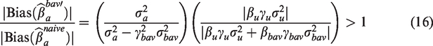
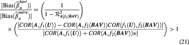
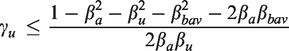
The magnitude of bias amplification can be potentially very large. From equations (8) and (9), the absolute bias of the BAV estimator will be larger than the absolute bias of the naive estimator whenever

$$\frac{|\text{Bias}({\widehat{\beta }}_a^{\mathit{bav}\prime })|}{|\text{Bias}({\widehat{\beta }}_a^{\mathit{naive}})|}=\left(\frac{{\sigma }_a^2}{{\sigma }_a^2-{\gamma }_{\mathit{bav}}^2{\sigma }_{\mathit{bav}}^2}\right)\left(\frac{\left|{\beta }_u{\gamma }_u{\sigma }_u^2\right|}{\left|{\beta }_u{\gamma }_u{\sigma }_u^2+{\beta }_{\mathit{bav}}{\gamma }_{\mathit{bav}}{\sigma }_{\mathit{bav}}^2\right|}\right)>1$$

(16)

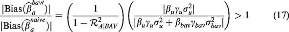
We can rewrite the first term on the right side of the equal sign as ${\left(1-{\mathcal{R}}_{A|\mathit{BAV}}^2\right)}^{-1}$ , which is the inverse of 1 minus percentage variance explained in A adjusting for BAV

$$\frac{|\text{Bias}({\widehat{\beta }}_a^{\mathit{bav}\prime })|}{|\text{Bias}({\widehat{\beta }}_a^{\mathit{naive}})|}=\left(\frac{1}{1-{\mathcal{R}}_{A|\mathit{BAV}}^2}\right)\left(\frac{\left|{\beta }_u{\gamma }_u{\sigma }_u^2\right|}{|{\beta }_u{\gamma }_u{\sigma }_u^2+{\beta }_{\mathit{bav}}{\gamma }_{\mathit{bav}}{\sigma }_{\mathit{bav}}^2|}\right)>1$$

(17)

Notice that the first term must always be greater than or equal to 1. The more strongly the control variables predict the treatment, the larger the magnitude of the term, increasing monotonically ¹¹ and hyperbolically in the treatment variance explained by BAV .

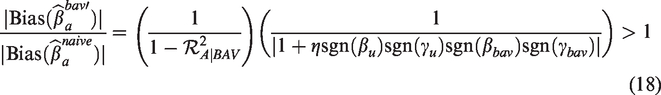
We now examine the second term after the equal sign. If ${\beta }_u=0$ or ${\gamma }_u=0$ , then there is no unmeasured confounding and ${\widehat{\beta }}_{\mathit{bav}}$ will be unbiased. If ${\beta }_u\ne 0$ and ${\gamma }_u\ne 0$ then there is unmeasured confounding, so by manipulating equation (17), we can write the second term as

$$\frac{|\text{Bias}({\widehat{\beta }}_a^{\mathit{bav}\prime })|}{|\text{Bias}({\widehat{\beta }}_a^{\mathit{naive}})|}=\left(\frac{1}{1-{\mathcal{R}}_{A|\mathit{BAV}}^2}\right)\left(\frac{1}{|1+\eta \text{sgn}({\beta }_u)\text{sgn}({\gamma }_u)\text{sgn}({\beta }_{\mathit{bav}})\text{sgn}({\gamma }_{\mathit{bav}})|}\right)>1$$

(18)

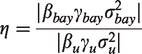
where $\text{sgn}(·)$ is equal to +1, −1, and 0 if the argument is positive, negative, and equal to 0, respectively, and η is defined as the ratio of the absolute strength of the confounding path through BAV $(|{\beta }_{\mathit{bav}}{\gamma }_{\mathit{bav}}{\sigma }_{\mathit{bav}}^2|)$ to the absolute strength of the confounding path through U $\left(\right|{\beta }_u{\gamma }_u{\sigma }_u^2\left|\right)$ .

$$\eta =\frac{\left|{\beta }_{\mathit{bay}}{\gamma }_{\mathit{bay}}{\sigma }_{\mathit{bay}}^2\right|}{\left|{\beta }_u{\gamma }_u{\sigma }_u^2\right|}$$

The second term depends on the signs of the structural coefficients for the two confounding paths. This is a dimensionless quantity that does not depend on the scale of the data, which can make it useful for sensitivity analysis. If ${\gamma }_{\mathit{bav}}=0$ , then BAV does not affect A , so it has no effect on the bias because η = 0 and ${\mathcal{R}}_{A|\mathit{BAV}}^2=0$ . In the special case that ${\beta }_{\mathit{bav}}=0$ , BAV is a true instrumental variable under the DAG in Figure 3. If there are no interactions as in the structural equations (4) and (5), then including an instrumental variable will always increase bias in the presence of unmeasured confounding.^3,10,14 We can see this clearly in equation (16) since by definition an instrumental variable does not explain variance in the outcome except through the treatment and must correlate with the treatment. A strong instrument in this case must be a strong amplifier since it will strongly predict variance in the treatment making the first term in equation (16) large and the second term exactly 1.

In the case that none of the structural coefficients are equal to 0, note that $\text{sgn}({\beta }_u)\text{sgn}({\gamma }_u)\text{sgn}({\beta }_{\mathit{BAV}})\text{sgn}({\gamma }_{\mathit{BAV}})$ will be equal to +1 if there is an even number of positive signs for the structural coefficients and it will be equal to −1 if there is an odd number of signs. We have defined η in terms of absolute values, so it must be non-negative. If $0\le \eta <1$ , then the confounding path through U is stronger than the path through BAV . If $\eta >1$ , then the confounding path through BAV is stronger than the path through U . When η = 1, the strengths of the two confounding paths are equal.

We can use equation (18) to characterize all possible confounding structures that lead to bias amplification. First assume that there are an even number of positively signed structural coefficients. This implies that the second term of equation (18) is equal to ${(1+\eta )}^{-1}$ and bias amplification will occur when ${(1-{\mathcal{R}}_{A|\mathit{BAV}}^2)}^{-1}>(1+\eta )$ or equivalently when $R_{A|\mathit{BAV}}^2{(1-R_{A|\mathit{BAV}}^2)}^{-1}>\eta$ . So if there is an even number of positively signed structural coefficients, the larger amount of treatment variance explained by BAV , the greater the range of possible η values that will lead to bias amplification.

Next assume that there is an odd number of positively signed structural coefficients, so that the second term will be equal to $|1-\eta {|}^{-1}$ . In this case, if $0<\eta \le 1$ (i.e. if the confounding path through U is stronger than the confounding path through BAV ), then there will always be bias amplification. If $\eta >1$ , then there will be bias amplification if ${(1-R_{A|\mathit{BAV}}^2)}^{-1}>(\eta -1)$ , similar to the case when $\eta >1$ .

In Appendix A.5 we further re-express η in terms of only correlations (or partial correlations if desired) and the coefficients of determination and free of model parameters. This is a dimensionless quantity that does not depend on the scale of the data, which can make it useful for sensitivity analysis. Additionally, the different ways of expressing the quantity can reveal portions of the unknown quantity which are estimable, i.e. functions of only observed data. Depending on the application parameters, it may be easier to express domain knowledge through correlations or percentage variance explained. This allows one to move more easily from one to the other, which should be very useful to applied researchers. We expand on these ideas in sections 5 and develop principled ways to simulate from such systems of equation. In Appendix A.5, we discuss exploiting the fact that correlations and variances are sufficient for determining the whole system of equations.

In summary, variable selection approaches which aggressively target confounding paths with strong associations with treatment and weak associations with outcome are at greater risk of bias amplification as they are much more sensitive to the assumption that a full sufficient set is measurable. Adding controlling variables in proportion to their ability to predict the treatment in linear models is only guaranteed to be bias reducing if the resulting selected variables satisfy ignorability assumptions. When this is not the case, we have shown that unmeasured confounding bias may be severely amplified since the treatment variance term increases both monotonically and hyperbolically. It is often not possible or extremely unlikely to select a sufficient set in many non-experimental settings, i.e. most investigators are not willing to assume their observational study is equivalent to a randomized trial. Thus the potential for bias amplification must be considered carefully.

4 Generalizing to a larger class of causal models

In sections (1) to (3), we showed examples of bias amplification under two different DAGs, each with linear structural equations in both the coefficients and variables and probability limit results under the DAG in Figure 3 and linear structural equations. In section 4.1 we extend bias amplification to the class of structural functions that are additive in the outcome and whose target causal effect is represented by β_a. In other words, we consider structural equations of the form

$$\mathit{Y}={\alpha }_y+\mathit{A}{\beta }_a+f_1(\mathit{U})+f_2(\mathit{BAV})+{ϵ}_{\mathit{1}}$$

(19)

$$\mathit{A}={\alpha }_a+g(\mathit{U},\mathit{BAV})+{ϵ}_{\mathit{2}}$$

(20)

We require minimal assumptions of treatment structural equation (20), in fact it is completely general except that it must be decomposable into a function of U and BAV (i.e. the $E[\mathit{A}|\mathit{U},\mathit{BAV}]={\alpha }_a+g(\mathit{U},\mathit{BAV})$ ) and an error term orthogonal to this function ( ${ϵ}_{\mathit{2}}:E[{ϵ}_{\mathit{1}}|\mathit{\iota },\mathit{U},\mathit{BAV}]=0$ ). For the outcome equation, we require more structure and assumptions on top of an orthogonal decomposition into the conditional expectation and error term ( ${ϵ}_{\mathit{1}}:E[{ϵ}_{\mathit{1}}|\mathit{\iota },\mathit{A},\mathit{U},\mathit{BAV}]=0$ ). Specifically we require that the outcome equation (19) is additive in functions of A , U , and BAV (ruling out interaction effects for example) and that the causal effect of interest is a single parameter β_a ( $\frac{\partial E[\mathit{Y|A},\mathit{U},\mathit{BAV}]}{\partial \mathit{A}}={\beta }_a$ ).

In section 4.2, we again consider the same structural setting, but extend the results and intuitions developed in sections 3 and 4.1 to more general orthogonalization techniques beyond least squares, namely a specific case of Neyman-Orthogonalization in partially linear models as used in double debiased approaches like in Chernozhukov et al. ¹⁷ We show that in both settings, we can decompose bias amplification into a component due to covariance between the treatment and the outcome through the confounding paths and a second term which is a ratio of marginal treatment variance to residual treatment variance after adjusting for other covariates. We can always estimate the residual treatment variance and should report these estimates in observational studies, particularly if variable selection was in part determined by strength of treatment prediction. As the remaining treatment variance decreases, the potential for bias amplification increases and any inferences about the causal effect depend more strongly on the assumption that unmeasured confounding is negligible. Further, similar to the earlier setting, we can directly estimate correlations, coefficients of determination, and conditional expectations composed only of observable variables. While the entire confounding pathways cannot be identified, some of the components can be. These estimable quantities, in turn, place restrictions on what the total confounding pathways can be. In section 5 we show how to use these principles and perform simulations to test the performance of competing estimators. In section 6 we apply these ideas to a real clinical data set.

4.1 Generalized bias amplification in least squares

If $f_2(\mathit{BAV})$ is known or can be well approximated (say by an appropriate basis expansion that grows in dimension as $n\to \infty$ ) up to a constant of proportionality and intercept, then in the limit there will not be any bias due to misspecification of $f_2(\mathit{BAV})$ (for a look at the case when $f_2(\mathit{BAV})$ is misspecified see Appendix section A.9.1). In such a case, we again can compare two feasible OLS estimators, the first being the Naive estimator ( ${\widehat{\beta }}_a^{\mathit{naive}}$ ) as before and the second the OLS estimator resulting from including $f_2(\mathit{BAV})$ or its approximation ( ${\widehat{\beta }}_a^{|f_2(\mathit{bav})}$ ). Under any DAG, it can be shown that under structural equations (19) and (20), there will be bias amplification when

$$\begin{array}{l}\frac{|\text{Bias}({\widehat{\beta }}_a^{\mathit{bav}\prime })|}{|\text{Bias}({\widehat{\beta }}_a^{\mathit{naive}})|}=\left(\frac{1}{1-{\mathcal{R}}_{\mathit{A}|f_2(\mathit{BAV})}^2}\right)\\ \times \left(\frac{|\mathit{COR}(\mathit{A},f_1(\mathit{U}))-\mathit{COR}(\mathit{A},f_2(\mathit{BAV}))\mathit{COR}(f_1(\mathit{U}),f_2(\mathit{BAV}))|}{|\mathit{COR}(\mathit{A},f_1(\mathit{U}))+\mathit{COR}(\mathit{A},f_2(\mathit{BAV}))\kappa |}\right)>1\end{array}$$

(21)

where $\kappa ={\sigma }_{f_2(\mathit{BAV})}{\sigma }_{f_1(\mathit{U})}^{-1}$ . In the above expression, we assume the case that there is in fact bias in the naive model, i.e. $\mathit{Bias}({\widehat{\beta }}_a^{\mathit{naive}})\ne 0$ .

Bias amplification is decomposed into two terms, the ratio of remaining variance in the treatment once the control variables are projected out, and the remaining covariance between the outcome and treatment through the confounding pathways. Just like in the linear case, the first term ${(1-{\mathcal{R}}_{A|f_2(\mathit{BAV})}^2)}^{-1}$ is the ratio of remaining treatment variance once we have projected out linear combinations of the control variables, which is just a constant in the naive case and $f_2(\mathit{BAV})$ in the adjusted case. This first term must be greater than 1 and is a hyperbolic function increasing as $f_2(\mathit{BAV})$ linearly explains more variance in the treatment.

Now consider the second bias term $\left(\frac{|\mathit{COR}(\mathit{A},f_1(\mathit{U}))-\mathit{COR}(\mathit{A},f_2(\mathit{BAV}))\mathit{COR}(f_1(\mathit{U}),f_2(\mathit{BAV}))|}{|\mathit{COR}(\mathit{A},f_1(\mathit{U}))+\mathit{COR}(\mathit{A},f_2(\mathit{BAV}))\kappa |}\right)$ which is the ratio of the covariance between the outcome and treatment remaining through the uncontrolled confounding pathways. The numerator of this expression ( $|\mathit{COR}(\mathit{A},f_1(\mathit{U}))-\mathit{COR}(\mathit{A},f_2(\mathit{BAV}))\mathit{COR}(f_1(\mathit{U}),f_2(\mathit{BAV}))|$ ) is the magnitude of the correlation between the treatment and $f_1(\mathit{U})$ once we have projected out linear combinations of BAV . When $f_1(\mathit{U})$ and $f_2(\mathit{BAV})$ are uncorrelated, or independent as they would be under the DAG in Figure 3 and equation (17) in section 3, then the numerator reduces to simply $|\mathit{COR}(\mathit{A},f_1(\mathit{U}))|$ since BAV does not linearly explain any of the shared variance in the treatment A and $f_1(\mathit{U})$ .

In general, when there is correlation between $f_1(\mathit{U})$ and $f_2(\mathit{BAV})$ , adjusting for $f_2(\mathit{BAV})$ reduces the confounding bias of $f_2(\mathit{U})$ when the signs of the correlations $\mathit{COR}(\mathit{A},f_2(\mathit{BAV}))$ and $\mathit{COR}(f_1(\mathit{U}),f_2(\mathit{BAV}))$ are the same. Otherwise, this adjustment may further increase the confounding bias. As a simple example, if all of the correlations are positive (i.e. $\mathit{COR}(\mathit{A},f_1(\mathit{U})),\mathit{COR}(\mathit{A},f_2(\mathit{BAV})),\mathit{COR}(f_1(\mathit{U}),f_2(\mathit{BAV}))>0$ then the second term in the amplification expression will be less than or equal to 1 ( $\left(\frac{|\mathit{COR}(\mathit{A},f_1(\mathit{U}))-\mathit{COR}(\mathit{A},f_2(\mathit{BAV}))\mathit{COR}(f_1(\mathit{U}),f_2(\mathit{BAV}))|}{|\mathit{COR}(\mathit{A},f_1(\mathit{U}))+\mathit{COR}(\mathit{A},f_2(\mathit{BAV}))\kappa |}\right)\le 1$ ). In this case, we reduce bias in two ways. First we remove the bias due to $\mathit{COR}(\mathit{A},\mathit{BAV})$ directly and then we reduce the remaining covariance between A and $f_1(\mathit{U})$ through the part of this correlation explained by BAV .

There will be amplification, on the other hand, if the first term (which is always greater than one) is bigger than the reciprocal of the second term (which in this case is less than one). If $\mathit{COR}(\mathit{A},f_1(\mathit{U}))$ and $\mathit{COR}(\mathit{A},{\mathit{f}}_{\mathit{2}}(\mathit{BAV}))$ are opposite signed, then when we adjust for BAV and remove bias due to the confounding path $\mathit{A}\leftarrow \mathit{BAV}\to \mathit{Y}$ we may increase bias since $\mathit{COR}(\mathit{A},f_1(\mathit{U}))$ and $\mathit{COR}(\mathit{A},f_2(\mathit{BAV}))$ would no longer be partially cancelling each other out as they do in the naive model. Similarly, projecting out linear combinations of BAV may increase or decrease the remaining covariance between the treatment and $f_1(\mathit{U})$ as seen in the numerator of the second term. Overall, this second term may be greater than or less than 1, meaning it may contribute to increasing or decreasing the bias relative to the naive estimator. By estimating the correlations and variances which are functions of observables and eliciting domain knowledge about the remaining unobserved quantities in the relative bias expression, we can make informed predictions about the plausibility of bias amplification.

Even in the most general case, where there are interactions and non-separability of U and BAV in the data generating model equation, the second term of the bias term will always be proportional to $1-{\mathcal{R}}_{A|Z}^2$ , where $\mathit{Z}=[\mathit{\iota },h(\mathit{BAV})]$ and $h(\mathit{BAV})$ are whatever function of BAV that we include in a regression. As can be seen in the appendix (section A.9.1), this is even true when we have misspecified $f_2(\mathit{BAV})$ . However, there will be an additional bias term due to misspecification, but this will also be amplified with respect to the denominator term. The overall lesson is that when using OLS for causal effect estimation, unmeasured confounding bias (and remaining misspecification bias) will be amplified hyperbolically with respect to how well the controlling variables linearly explain variance in the treatment, i.e. the magnitude of ${\mathcal{R}}_{A|Z}$ , where Z is all of the variables that are not A that we include in our OLS regression. Further, it is important to note that the amplifying factor ( ${(1-{\mathcal{R}}_{A|f_2(\mathit{BAV})}^2)}^{-1}$ ) is always a function of only observables and can always be estimated by running the regression A on $f_2(\mathit{BAV})$ . We can use these estimates for sensitivity analysis or in a model selection procedure. In a case like the simulation in Figure 2, our potential controls explain the large majority of the treatment variance. When this occurs, we should require more confidence that there is no unmeasured confounding after adjusting for our controls before we trust these estimates.

When there are causal pathways between U and BAV , we showed that this may help make the first term smaller. However, this will open up an additional pathway for $f_2(\mathit{BAV})$ to explain variance in the treatment (for example $\mathit{BAV}\to \mathit{U}\to \mathit{A}$ as in the DAG in Figure 1, but in general the path could be indirect or the direction of causation may be reversed) and thus make the second hyperbolic term larger. This was the source of the dramatic bias amplification in Figure 2 simulated under linear structural equations from the DAG in Figure 1. In that specific case, BAV was a very good proxy for the unmeasured confounding U and this has two effects. First, it means that including BAV eliminates the large majority of the unmeasured confounding through its path to the outcome. Second, this means that BAV linearly explains nearly as much variation in the treatment as including both BAV and U , which is nearly all of the variation in the treatment in that simulation case. So the little unmeasured confounding remaining was amplified significantly, more than 25 times $\left({((1-{\mathcal{R}}_{A|\mathit{BAV}}^2){\sigma }_a^2)}^{-1}={({\sigma }_a^2-{\displaystyle {\sum }_{i=1}^{10}{({\gamma }_{\mathit{bav}}{\hspace{0.17em}}_i+{\gamma }_u{\hspace{0.17em}}_i{\psi }_{\mathit{bav}}{\hspace{0.17em}}_i)}^2}{\sigma }_{\mathit{bav}}^2{\hspace{0.17em}}_i)}^{-1}={(1-0.96015)}^{-1}=25.09725\right)$ under the DAG in Figure 1 and linear structural equations (1) to (3)). This is because the potential amplifier linearly explained more than 96% of the variance in the treatment.

4.2 Bias amplification in more general semi-parametric models

In the beginning of this paper, we considered bias amplification in the context of linear expectations and linear models. In section 4.1 we extended this to when the structural models are non-linear when the estimator is ordinary least squares. Here we show proof of concept for bias amplification in more general semi-parametric orthogonalization methods. We plan to further develop this work in the future. We again consider the underlying structural equations to be represented by equations (19) and (20).

In the case that ${\mathit{f}}_{\mathit{2}}(\mathit{BAV})$ is unknown, one might turn to more general semi-parametric estimators for the causal effect estimation. A reasonable semi-parametric estimator for these structural equations is Robinson’s Double Residual Regression (DRR hereforth) ¹⁸ when the outcome is hypothesized to be linear in the treatment (or well approximated by a partial linear function). In section 3 we showed via the FWL theorem that we can think of multiple regression as simple regression of the outcome and treatment once linear combinations of the control variables (which may be non-linear functions themselves as shown in section 4.1) have been projected out. In other words, we orthogonalized the outcome and treatment with respect to the subspace spanned by the linear combinations of all the control variables we included in our regression model ( Z ) and then perform simple linear regression on the orthogonalized variables. The coefficient of interest in DRR, just like in multiple linear regression, is the result of a least squares estimate of an orthogonalized outcome and treatment, but we orthogonalize with respect to a more general subspace using the expectation operator.

Considering some arbitrary random variable Y and collection of controls ${\mathit{X}}_{\mathit{1}},\dots ,{\mathit{X}}_{\mathit{n}}$ (each with finite variance), the conditional expectation $E[\mathit{Y|}{\mathit{X}}_{\mathit{1}},\dots ,{\mathit{X}}_{\mathit{n}}]$ is the projection of Y onto a closed subspace of ${\mathcal{L}}^2$ consisting of all Borel functions $\varphi ({\mathit{X}}_{\mathit{1}},\dots ,{\mathit{X}}_{\mathit{n}}):{\mathcal{R}}^n\to \mathcal{R}$ , see for example Brockwell and Davis. ¹⁹ This is the heart of the familiar result that the conditional expectation is the function of ${\mathit{X}}_{\mathit{1}},\dots ,{\mathit{X}}_{\mathit{n}}$ which minimizes the mean-squared error ( $\underset{f:{\mathcal{R}}^n\to \mathcal{R},\text{ Borel }}{\text{argmin}}E[{(\mathit{Y}-\mathit{f}({\mathit{X}}_{\mathit{1}},{\mathit{X}}_{\mathit{2}},\dots ,{\mathit{X}}_{\mathit{n}}))}^2]=E[\mathit{Y|}{\mathit{X}}_{\mathit{1}},{\mathit{X}}_{\mathit{2}},\dots ,{\mathit{X}}_{\mathit{n}}]$ ). The set of linear functions is a strict subset of all Borel functions, making conditional expectation a more general projection than the projections implicit in least squares estimation. In other words, if it turns out that the conditional expectations for both Y and A are in fact linear in the same variables, the DRR estimator will be equivalent to OLS in the probability limit.

The first step of DRR is to estimate the conditional expectations, i.e. the projections, $E[\mathit{Y|BAV}]$ and $E[\mathit{A|BAV}]$ . We can use our favorite non-parametric estimator(s) as long as it is consistent as $n\to \infty$ . It is common to use a conditional density estimator, but one may choose to use modern regression tree models or machine learning techniques like neural networks as in the context of Chernozhukov et al.. ¹⁷ Now we construct our orthogonalized outcome and treatment, $\tilde{\mathit{Y}}=\mathit{Y}-\widehat{E}[\mathit{Y|BAV}]$ and $\tilde{\mathit{A}}=\mathit{A}-\widehat{E}[\mathit{A|BAV}]$ . Finally, we perform least squares of the modified outcome ( $\tilde{\mathit{Y}}$ ) on the modified treatment ( $\tilde{\mathit{A}}$ ) to get our semi-parametric estimator denoted ${\widehat{\beta }}^{\mathit{semi}}$ .

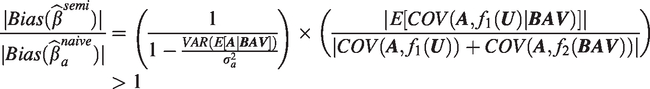
Bias amplification will occur in the probability limit when

$$\frac{|\mathit{Bias}({\widehat{\beta }}^{\mathit{semi}})|}{|\mathit{Bias}({\widehat{\beta }}_a^{\mathit{naive}})|}=\left(\frac{1}{1-\frac{\mathit{VAR}(E[\mathit{A|BAV}])}{{\sigma }_a^2}}\right)\times \left(\frac{|E[\mathit{COV}(\mathit{A},f_1(\mathit{U})|\mathit{BAV})]|}{|\mathit{COV}(\mathit{A},f_1(\mathit{U}))+\mathit{COV}(\mathit{A},f_2(\mathit{BAV}))|}\right)>1$$

Once again, we can decompose this relative bias expression into two components. The first term is the ratio of remaining treatment variance once the controlling variables have been projected out of the treatment and the second term $\left(\frac{|E[\mathit{COV}(\mathit{A},f_1(\mathit{U})|\mathit{BAV})]|}{|\mathit{COV}(\mathit{A},f_1(\mathit{U}))+\mathit{COV}(\mathit{A},f_2(\mathit{BAV}))|}\right)$ is the ratio of confounding covariances remaining through the outcome paths $\mathit{U}\to \mathit{A}\to \mathit{Y}$ and $\mathit{BAV}\to \mathit{A}\to \mathit{Y}$ . The first term again always contributes to amplification, since ${(1-\mathit{VAR}(E[\mathit{A|BAV}])/{\sigma }_a^2)}^{-1}\ge 1$ . This is the direct analogue of the results developed in the previous sections. In this case, ${\mathcal{R}}_{A|\mathit{BAV}}^2$ is the variation of the treatment explained by linear combinations of BAV (or $h(\mathit{BAV})$ if we have included a different function of BAV in our regression), and $\mathit{VAR}(E[\mathit{A|BAV}]){\sigma }_a^{-2}$ is the total variation explained by fluctuations in BAV . ²⁰ As before, the first term increases hyperbolically as BAV explains more treatment variance.

When we project out BAV , the term $\mathit{COV}(\mathit{A},f_2(\mathit{BAV})$ drops from the second component and $\mathit{COV}(\mathit{A},f_1(\mathit{U}))$ becomes $E[\mathit{COV}(\mathit{A},f_1(\mathit{U})|\mathit{BAV})]$ . Depending on the signs of the bias and the direction of the correlation $\mathit{COV}(E[\mathit{A|BAV}],E[f_1(\mathit{U})|\mathit{BAV}])$ , the second term may be greater or less than 1. This is similar to the first term in the expression in equation (21) since the biases from the two confounding paths may partially cancel each other out and thus by projecting them both out, one may increase bias.

In other words, the underlying mechanics of bias amplification extends to more general orthogonalization methods, both explicit as in the case of DRR and implicit like that in OLS. In particular, the partially linear regression set-up is the basis for more complicated causal machine learning techniques such as Double Machine Learning residuals on residuals regression, ¹⁷ which has become a popular approach for dealing with regularization bias in high dimensional settings. Even in these more complicated settings where we orthogonalize in more sophisticated ways, variables which predict large amounts of variance in the treatment may significantly increase bias if confounding pathways remain. Once again, the hyperbolic remaining treatment variance term is entirely a function of observed variables and thus can be estimated (non-parametrically if desired) to see if one is at risk of bias amplification with respect to priors or sensitivity analysis over expected levels of unmeasured confounding. Similarly, we can use the mean-squared error of our resulting model to evaluate the extent to which unmeasured confounding is possible through the outcome path since no interaction implies that remaining variation must either be independent error or unmeasured confounding. A full treatment of this framework is beyond the scope of this article and will be the subject of future work.

5 Causal simulation experiments: the case of bias amplification

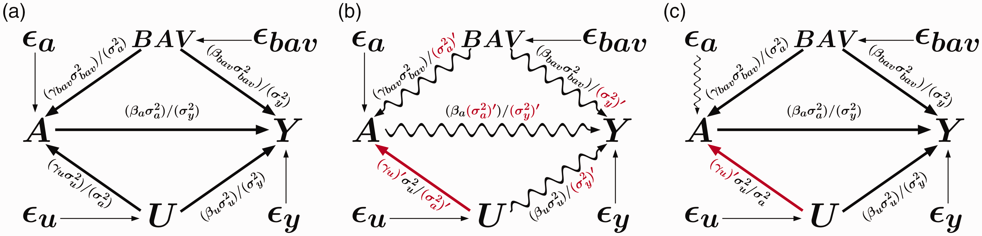
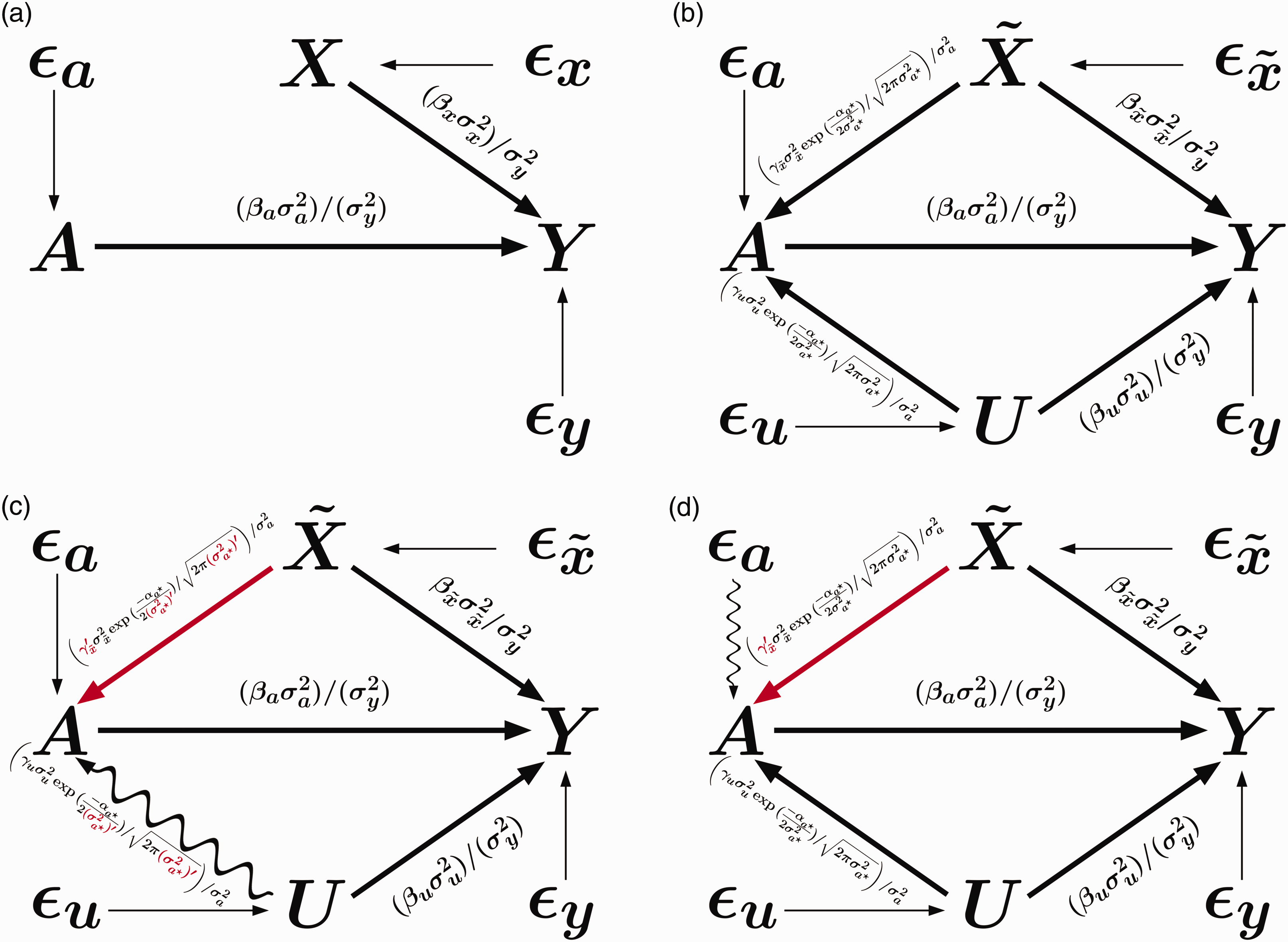
In our experience, simulating bias amplification is challenging in a number of subtle, but important ways. Our context of interest is assessing the potential for bias amplification in an analysis of an observational study in which we have measured several independent variables and the outcome but there might be an unmeasured confounder. We are interested in evaluating the feasible estimators we have developed in the previous sections, ${\widehat{\beta }}_a^{\mathit{naive}}$ and ${\widehat{\beta }}_a^{\mathit{bav}\prime }$ for example, with respect to possible data sets generated by a class of DAGs and structural equations. In this section, we show that if we constrain certain aspects of the simulated data (in particular, the marginal variances of observed quantities), we are better able to articulate and answer causal questions about the effect of bias amplification on proposed estimators. While we discuss the example of bias amplification simulations specifically, this section has implications for simulating data to test causal estimators more broadly. Now, consider the challenge of determining the effect of increasing unmeasured confounding on bias amplification in Figure 5(a). We might, for example, be interested in how large an unmeasured confounder must be, with fixed amplifying variables, to cross some threshold of bias in the adjusted model as part of a sensitivity analysis. To answer such a question, we must define clearly what is meant by the strength of an unmeasured confounder. In Figure 5(a), there are two edges which determine the overall bias due to the unmeasured confounding path through U: the edge from U to A and the edge from U to Y . The bias due to the unmeasured confounding path through U in the naive model is simply the product of the weight of these two edges, scaled by the variance of the treatment as shown in equation (7). The extent to which bias can become amplified, however, is not symmetric with respect to the weight of the edges $\mathit{U}\to \mathit{A}$ and $\mathit{U}\to \mathit{Y}$ , since amplification is the result of variance explained in the treatment as discussed in section 3. There is more potential for amplification of a strong unmeasured confounder (in the sense the product of the confounding edges is large) when the strength is due to U being a strong cause of Y compared to a strong cause of A . This is because when U is a strong cause of A , the BAV can only explain a small amount of the variance of A , limiting the possible amount of bias amplification. Thus, to answer a causal question about the effect of increased unmeasured confounding on bias amplification, we should only vary one of the confounding edges, holding all other edges fixed.

Figure 5.

Causal diagrams where (a) represents the underlying causal structure. In addition to the usual causal pathways, we explicitly show the pathway of the independent error terms, ${ϵ}_a,{ϵ}_u,{ϵ}_{\mathit{bav}},{ϵ}_y$ . (b) The simulation experiment where we change strength of the edge $\mathit{U}\to \mathit{A}$ (shown in bold red) and do not renormalize the variance of the treatment ( A ). All edges which have been inadvertently modified are symbolized as squiggly arrows. All parameters which have been modified (inadvertently or intentionally) are shown in red along the edges. (c) Intervening on $\mathit{U}\to \mathit{A}$ , where the variance of the treatment is fixed. To do so, we modify the variance of the noise term ϵ_a, visualized by the squiggly arrow. Notice no other edges are inadvertently modified.

As an example, suppose we are interested in the change in bias amplification when we increase the strength of the edge from U to A , holding all else constant. This notion of intervening on a single edge of our DAG while holding the others fixed should be familiar to causal inference practitioners since it is the principle behind counterfactual analysis more broadly. Here we want to ensure that our results from varying a single edge are not confounded by variations in other edges as the result of unintended consequences or induced associations.

Because the goal is to increase the strength of a single edge, holding all else constant, we must specify a metric by which we measure the strength of the edge. In a fully linear system, we might consider the strength of the edge as the regression coefficient itself, γ_u, or the proportion of variance explained by U , $\frac{{\gamma }_u^2{\sigma }_u^2}{{\sigma }_a^2}$ and the sign of γ_u. It is tempting to see the two measures as equivalent with different scalings, but this is only true in the context of simulating a single equation. In the context of a system of linear equations, especially with the potential for bias amplification, we argue the relevant quantity is the proportion of variance explained by each child node of the parent variable. This can be seen most easily by examining the bias formula in equation (11), where the denominator is the remaining variation in A unexplained by the potential bias amplifying variables.

Consider the implications of treating the coefficients themselves as the relevant measure of edge strength in a simulation trying to determine the effect of increasing the causal association along the path from U to A . If we want to increase γ_u to ${\gamma }_u\prime >{\gamma }_u$ without changing any other parameters, we must also increase the total variance in the treatment, A , since ${\sigma }_a^2={\gamma }_u^2{\sigma }_u^2+{\gamma }_{\mathit{bav}}^2{\sigma }_{\mathit{bav}}^2+{\sigma }_{{ϵ}_2}^2$ . A treatment with a larger variance is in some sense a different intervention, and thus this simulation is not compatible with the class of experiments which generated the original data with parameter γ_u. Further, from the previous sections we know this implies the total amount of variance explained from the bias amplifier BAV is reduced, since $\frac{{\gamma }_{\mathit{bav}}^2{\sigma }_{\mathit{bav}}^2}{({\sigma }_a^2)\prime }$ has been reduced. Although we have not changed the parameter γ_bav we have decreased the extent to which BAV amplifies the bias as seen by examining equation (11). The increased variance in A in turn modifies the total variance of Y . Therefore, the relative proportion of variance of Y that is explained by BAV is modified by changing the causal effect of $\mathit{U}\to \mathit{A}$ , as are the measured proportion of variance of $\mathit{BAV}\to \mathit{A},\mathit{A}\to \mathit{Y},\mathit{U}\to \mathit{Y}$ , and $\mathit{BAV}\to \mathit{Y}$ and their associated covariance terms.

We can see in Figure (5(b)) that by modifying a single coefficient and leaving all other coefficients unchanged we have inadvertently modified the relative proportion of variance explained by the four other edges ( $\mathit{BAV}\to \mathit{A},\mathit{BAV}\to \mathit{Y},\mathit{U}\to \mathit{Y}$ , and $\mathit{A}\to \mathit{Y}$ ) represented by the wavy arrows. Data generated by the second set of structural equations are not compatible with the constraints of the experiment which generated the first data and by intervening on a single edge we have modified all of the competing effects of interest. Comparing the distribution of estimates produced under γ_u and ${\gamma }_u^{\prime }$ gives us a confounded and thus biased estimate of the impact of increasing the unmeasured confounding through its causal pathway to the treatment on the estimators or functions thereof. We will show that this bias can result in under-estimating the impact of bias amplifying variables.

In general, when we vary one of the regression coefficients along a causal pathway, this has upstream and downstream effects on the proportion of variance explained by all variables going into or out of the varied node. In order to keep the proportional effects of the other edges constant, we need to use the error terms of the structural equations ( ${ϵ}_{\mathit{1}}$ and ${ϵ}_{\mathit{2}}$ ) to absorb the shocks to the marginal variances.

In Figure 5(c), if we change γ_u and simply adjust the structural error term ϵ_a such that the total variance in A remains constant, we can isolate the effect of modifying $\mathit{U}\to \mathit{A}$ . In Figure 6(a) we visualize the consequences of failing to hold the variance of the treatment when we modify γ_u. In red, for Figure 6(a), we simulate bias amplification where ${\gamma }_u=0.3$ . In green, we simulate bias amplification where γ_u is increased to 0.55 holding all other parameters constant, thus allowing the total variance of the treatment to grow from 1 to 1.21. This has the downstream effect of also increasing the variance of the outcome from 1 to 1.02. This also then impacts the relative proportions of variance explained of the treatment and the outcome that are explained by U and BAV , respectively. Notice that the bias increases from 20% ( $\frac{0.36-0.3}{0.3})$ to 43% $(\frac{0.43-0.3}{0.3})$ . In blue, we increase γ_u from 0.3 to 0.55, but re-normalize the variance in the treatment to remain constant at 1. The bias now increases further to 67% ( $\frac{0.5-0.3}{0.5}$ ) with respect to the original simulation in red. We do this by decreasing the variance of the independent noise term, ${ϵ}_{\mathit{a}}$ to ${ϵ}_{\mathit{a}}^{\prime }$ , allowing it to absorb the increase in variation from U . When we do not fix the variance, we underestimate the impact of the amplifier on both the bias and the variance because the unfixed variance case simulates a different kind of intervention due to the change in variance of the treatment variable. In the simulation above, by not keeping the variance fixed in A we implicitly reduced the amount of variance that BAV accounts for in the treatment from 36% to 30%. In effect, we were comparing the distribution of

$$P(\widehat{{\beta }_a}|{\gamma }_u\prime ,{\gamma }_{\mathit{bav}},{\beta }_u,{\beta }_a,{\beta }_{\mathit{bav}})$$

$$\text{ to }$$

$$P(\widehat{{\beta }_a}|{\gamma }_u,{\gamma }_{\mathit{bav}},{\beta }_u,{\beta }_a,{\beta }_{\mathit{bav}})$$

Figure 6.

(a) Simulation results from the experiment of intervening on the edge $\mathit{U}\to \mathit{A}$ . The ground truth, ${\beta }_a=0.2$ , is visualized by the black vertical line. In red we visualize the baseline bias amplification. Green shows the results of the conditional estimator in the case where we increase the weight of the edge, but fail to fix the variance of the treatment, allowing it to grow. In blue, we show the bias when we increase the weight of the edge but now hold the variance constant so the variances remain compatible with the original data. (b) Simulation results from the same experiment as (a) but the outcome is the difference in absolute bias between the conditional estimator ${\widehat{\beta }}_a^{\mathit{bav}\prime }$ and the naive estimator ${\widehat{\beta }}_a^{\mathit{naive}}$ . A value greater than zero (black vertical line) indicates that the conditional estimator was more biased than the naive estimator. Parameter values: ${\beta }_a=0.2,{\beta }_u=0.3,{\beta }_{\mathit{bav}}=-0.05,{\gamma }_{\mathit{bav}}=0.6$ .

when a more fair causal counterfactual would be to compare the distribution of

$$P(\widehat{{\beta }_a}|(\mathit{U}\to \mathit{A})\prime ,\mathit{U}\to \mathit{Y},\mathit{BAV}\to \mathit{A},\mathit{BAV}\to \mathit{Y},\mathit{A}\to \mathit{Y})$$

$$\text{ to }$$

$$P(\widehat{{\beta }_a}|\mathit{U}\to \mathit{A},\mathit{U}\to \mathit{Y},\mathit{BAV}\to \mathit{A},\mathit{BAV}\to \mathit{Y},\mathit{A}\to \mathit{Y})$$

Therefore, our simulation experiment results in green are distorted because when we increased the unmeasured confounding through $\mathit{U}\to \mathit{A}$ , we also decreased the strength of the bias amplifying variable through the pathway $\mathit{BAV}\to \mathit{A}$ . Notice that this bias will impact decisions and conclusions we might make about the merits of different estimators in this context. For example, below we compare the conditional estimator, ${\widehat{\beta }}_a^{\mathit{bav}\prime }$ , to the naive estimator, ${\widehat{\beta }}_a^{\mathit{naive}}$ with respect to their bias in the same three simulation set ups.

In Figure 6(b) we show the direct comparison of the bias for the conditional and the naive estimators. When we increase the unmeasured confounding through γ_u but fail to renormalize the treatment variance, we do not capture the full extent to which the conditional estimator amplifies the bias. If we compare the green and red plot, it would seem that nearly doubling the unmeasured confounding coefficient only has a small impact on the relative bias of the naive and conditional estimator, since the relative bias only increased from 0.07 to 0.09 (29%). By comparing the green density plot to the blue, we see the relative bias doubles (from 0.07 to 0.14). Therefore, the decision to use the naive or conditional estimator is in fact much more sensitive to the amount of unmeasured confounding than it would appear under the improper simulation with floating variance. It is extremely important to do these kinds of simulations properly particularly in the context of sensitivity analysis where we are testing the performance of estimators with respect to untestable assumptions such as unmeasured confounding.

To properly simulate bias amplification and answer questions of clinical concern with respect to the merits of potential estimators, we must think of the structural equations as an interconnected system. While we typically specify such equations from the perspective of determining their conditional means, the structural equations along with our independence assumptions determine the variances of the variables in the system. Above, this necessitates increasing the strength of the edge $\mathit{U}\to \mathit{A}$ while holding all other edges constant, which requires us to re-normalize the variances to maintain the strength of the edge $\mathit{BAV}\to \mathit{A}$ .

In Appendix section A.10, we consider the properties of a simulation experiment aiming to vary the strength of the edge $\mathit{BAV}\to \mathit{A}$ . We show that in the case that we fail to fix the variance of the treatment that the bias of the conditional estimator ${\widehat{\beta }}_a^{\mathit{bav}\prime }$ is invariant to ${\gamma }_{\mathit{bav}},\forall {\gamma }_{\mathit{bav}}\in (-\infty ,\infty )$ , but that the naive estimator is strictly increasing in γ_bav. It is clear from the theory we developed in section 3 that if we increase the edge from $\mathit{BAV}\to \mathit{A}$ that amplification should strictly increase, but if we allow the variance in A to increase as the parameter increases, the amplification effect is precisely cancelled out.

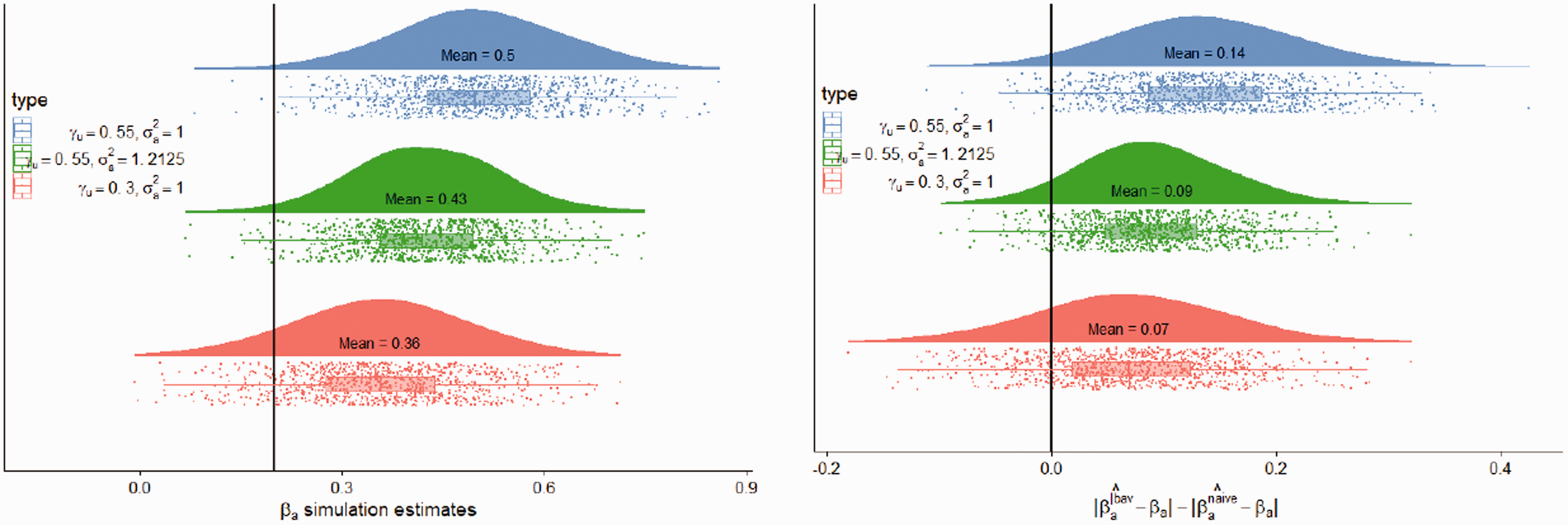
In general terms, simulating linear systems of location-scale family random variables requires first fixing the variances of the variables in the DAG. The relevant quantity determining the strength of the various edges are ratios of variances and covariances of the upstream parent nodes to the variance of the child node in determining the edge’s strength. Since the effects are relative, in a simulation context we can normalize the variances to 1 or set them to the expected/observed variances of the data in a particular context. For simplicity we will demonstrate the normalized approach. In Figure 3, this means that ${\sigma }_u^2={\sigma }_a^2={\sigma }_{\mathit{bav}}^2={\sigma }_y^2=1$ .

The second step is to be explicit about independence and conditional independence assumptions. Given the independence assumptions, we can specify the covariance matrix of each child variable ${\mathit{Y}}_{\mathit{child}}$ in terms of the matrix of k arbitrary parent variables which form the edges going into the child variable, ${\mathit{Y}}_{\mathit{child}}$ .

$${\mathit{Y}}_{\mathit{child}}={\mathit{X}}_{\mathit{parent}}{\mathit{\beta }}_{\mathit{parent}}+{ϵ}_{\mathit{child}}$$

$$\mathit{Var}(Y_{\mathit{child}})={\mathit{\beta }}_{\mathit{parent}}^{\mathit{T}}\mathit{Var}({\mathit{X}}_{\mathit{parent}}){\mathit{\beta }}_{\mathit{parent}}+\mathit{Var}({ϵ}_{\mathit{child}})$$

$${\sigma }_{y_{\mathit{child}}^2}=1=\left[\begin{array}{ccc}{\beta }_1& {\beta }_2& \dots {\beta }_k\end{array}\right]\left[\begin{array}{cccc}1& {\sigma }_{1,2}& \dots & {\sigma }_{1,k}\\ {\sigma }_{1,2}& 1& \dots & {\sigma }_{2,k}\\ ⋮& {\sigma }_{j,2}& \ddots & ⋮\\ {\sigma }_{k,1}& {\sigma }_{k,2}& \dots & 1\end{array}\right]\left[\begin{array}{c}{\beta }_1\\ {\beta }_2\\ ⋮\\ {\beta }_k\end{array}\right]+{\sigma }_{{ϵ}_c}^2$$

The diagonal of all the parent covariance matrices is 1 since we have normalized all variables pictured in the DAG. The covariances themselves will be determined by the independence assumptions, the edges connecting the child nodes, and their structural equations. Essentially we are choosing the proportion of the child variation that the variances and the covariances of the parent variances explain. The error terms, ϵ’s are the only non-normalized variances, and they absorb the shocks when we increase and decrease the strength of the edges of the non-error variables. This maintains the strength of all other relations visualized on the DAG.

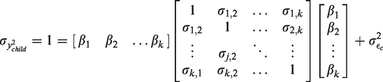
Since all variance terms must be non-zero (or equivalently that ${\mathit{\beta }}_{\mathit{parent}}^{\mathit{T}}\mathit{Var}({\mathit{X}}_{\mathit{parent}}){\mathit{\beta }}_{\mathit{parent}}\le 1={\sigma }_{\mathit{child}}^2$ ), the variance equations define bounds on the simulation parameter space. In the above example, conditional on holding the strength of the edges $\mathit{U}\to \mathit{Y},\mathit{BAV}\to \mathit{A},\mathit{BAV}\to \mathit{Y},\mathit{A}\to \mathit{Y},{\gamma }_u\in (-0.893,0.893)$ defines the feasible range. That is, the edge $U\to A$ can explain up to 79.75% of the variation in A ( $\frac{{\gamma }_u^2{\sigma }_u^2}{{\sigma }_a^2}=\frac{{\gamma }_u^2}{1}$ ) since the edge $\mathit{BAV}\to \mathit{A}$ explains 20.25% of the variation already. In general, the extent to which an edge can explain variation in the child node is constrained by the other child nodes and the covariance structure between those variables. A parameter, however, such as γ_u may be constrained by more than one set of inequalities. In this particular case, γ_u has to satisfy the following inequalities

$$\left|{\gamma }_u\right|\le {(1-{\gamma }_{\mathit{bav}}^2)}^{\frac{\hspace{0.17em}}{12}}$$

$${\gamma }_u\le \frac{1-{\beta }_a^2-{\beta }_u^2-{\beta }_{\mathit{bav}}^2-2{\beta }_a{\beta }_{\mathit{bav}}}{2{\beta }_a{\beta }_u}$$

where conditional on the strength of the particular edges ( $\mathit{U}\to \mathit{Y},\mathit{BAV}\to \mathit{A},\mathit{BAV}\to \mathit{Y},\mathit{A}\to \mathit{Y}$ ) in the above simulation, only the first inequality was binding.

The nuance here is that the extent to which we can simulate unmeasured confounding depends upon not only how much amplifying we have simulated, but also on the true effect of the treatment on the outcome $\mathit{A}\to \mathit{Y}$ . Since this is an interdependent system of equations, all of the parameters are competing for shares of fixed variances. If the treatment, independent of U and BAV , explains the large majority of the outcome variance (i.e. the edge $\mathit{A}\to \mathit{Y}$ ), it means the weight of the edge $\mathit{U}\to \mathit{Y}$ must be relatively small, opposite signed, or the structural equations contain an effect modifier. This in turn constrains γ_u.

Consider again the above simulation experiment where we are interested in varying the strength of $\mathit{U}\to \mathit{A}$ conditional on all other pathways. Suppose that the pathway $\mathit{A}\to \mathit{Y}$ explains 64% of the variance in Y , i.e. that ${\beta }_a=0.8$ . Now both constraints on γ_u are binding and the simulation parameter space is ${\gamma }_u\in (-0.893,0.3916)$ .

In summary, when simulating linear location-scale family systems of equations, we start by identifying the DAG and the independence assumptions between variables. Second, our simulation experiment should attempt to answer a causal question about how a proposed estimator behaves in response to an intervention on the weights of causal DAG. Just like experimental design, properly estimating the relevant counterfactual requires that the difference in distributions between our intervention(s) and the control is the effect of the intervention(s) themselves. As demonstrated in this section, simulating linear systems of equations requires varying one of the edges of the DAG holding all else constant, and matching the means and variances of the simulated variables with that of the target observational study we are trying to mimic. This allows us to generate simulations whose distributions are proper counterfactuals. Third, conditional on the other edges, the covariance matrices impose bounds for the parameter space that we can simulate and thus the extent to which we can vary the edge of interest. For a specific realization of the experiment and accompanying valid parameters, the variables are constructed in the downstream direction, that is from parent nodes to child.

In the example of simulating the proper intervention in Figure 5(c), we first simulate U and BAV independently with variance 1, respectively. Given γ_u and γ_bav, the variance of the error term ${ϵ}_{\mathit{2}}$ from equation (5) is implied and can be simulated. Having U , BAV and ${ϵ}_{\mathit{2}}$ allows us to simulate the treatment A . Conditional on the already simulated variables, their associated parameters, and β_a, β_bav, and β_u, the variance of the error term ${ϵ}_{\mathit{1}}$ is implied and can be simulated. Finally, since all of the child variables for the outcome have been simulated, we can simulate the outcome. To be clear, we can fix proportions of variance explained by each edge in any order we’d like as long as we respect the underlying constraints. However, given an admissible set of weights of the edges we must proceed from parent to child nodes to conduct the simulation.

While this method requires us to calculate inequalities and make explicit the implied variance formulas for our variables, the benefits are that we can view our simulation as a well-defined causal experiment matching the constraints of our target study and we get sets of parameter bounds. When we do not keep the variance fixed, there are no defined bounds beyond heuristics, and more importantly, we are no longer matching the data to our target observational study. In many small systems, such as the one in Figure 5(a), it is often computationally inexpensive to simulate a discretized approximation to all possible parameter configurations. In extremely large systems, we can use domain knowledge to make refinements on these bounds and simulate a reasonable subset of the parameter space. This method allows us to make refinements over edges with strong priors while simulating the entirety of edges with greater uncertainty.

An alternative, but equivalent way of developing a causal simulation for linear systems of equations would be to work with correlation (or covariance) matrices and variances directly as opposed to parameters. In the Appendix section A.5, we discuss representations of regression coefficients and linear structural parameters in terms of partial correlations, correlations, and coefficients of determination. In some cases, it may be easier to elicit domain knowledge using partial correlations or correlations, compared to the parameters themselves, depending on the clinician and the application at hand. There are still constraints on the system, which are implied by the constraints of a non-singular correlation matrix. One of the potential benefits of working directly with the correlation matrix is that, as shown in section A.5 much of the pairwise correlation matrix can be directly estimated form the observed data. Further, there exist methods to augment the estimable portion of the matrix to a non-singular full correlation matrix as well as methods to add noise to a valid correlation matrix to represent the uncertainty inherent in the estimation process. Additionally, sometimes causal DAGs may imply further restrictions on correlation matrices (or partial correlation matrices) and thus the underlying regression parameters and causal effects.

6 Simulating bias amplification from a real data set

Here we conduct a data simulation for an observational study. We want to consider a medical example with realistic amounts of variance in the treatment and the outcome. Further, we specifically consider the case of a binary treatment which is common in medical applications, biostatistics, and epidemiology. The difficulty, in general, when working with real data in the spirit of plasmode simulation^21,22 is that you do not know the true underlying parameter values. In this section, we start with a randomized controlled trial (RCT) and modify it appropriately, so that we can take the intention to treat (ITT) estimate as the true underlying effect for the foundation of our simulations.

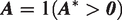
In our simulation experiment, we keep the treatment data unchanged (thus fixing their variance), and then simulate unmeasured confounding ( U ) and bias amplifiers ( BAV ) in order to modify selected covariates ( X ) and the outcome ( Y ) to produce a synthetic observational experiment. In order to precisely control the relationships between the simulated variables and the real variables, we treat the binary treatment, A , as though it comes from a latent probit model.

$$\mathit{A}=1({\mathit{A}}^{*}>\mathit{0})$$

$$\hspace{1em}\hspace{1em}\hspace{1em}\hspace{1em}\hspace{1em}\hspace{1em}\hspace{1em}\hspace{1em}\hspace{1em}=1({\alpha }_a+\mathit{U}{\gamma }_u+\tilde{\mathit{X}}{\gamma }_{\tilde{x}}+{ϵ}_{\mathit{2}}>\mathit{0})$$

where $\tilde{\mathit{X}}=\frac{\mathit{X}}{\sigma \prime }+\mathit{BAV}$ , and $\sigma \prime$ is a scaling variable such that X and $\tilde{\mathit{X}}$ have the same population variance. All of the latent variables ( U , $\mathit{BA}{\mathit{V}}_{\mathit{n}\times \mathit{k}},{ϵ}_{\mathit{2}}$ , and hence ${\mathit{A}}^{*}={\alpha }_a+\mathit{U}{\gamma }_u+\mathit{BAV}{\gamma }_{\mathit{bav}}+{ϵ}_{\mathit{2}}>\mathit{0}$ ) are set to come from normal distributions. The details of the how the simulation is performed are in Appendix section A.11.

For this paper, we use data from Helle et al., ^23,38,39 a published RCT with 294 participants and relatively balanced distribution of covariates. While the researchers examined many outcomes, we will focus on the effects of an e-Health intervention in infants on child eating behaviors. The researchers gave the parents in the treatment group access to a “monthly age-appropriate video addressing infant feeding topics together with corresponding cooking films/recipes,” and the outcome was eating habits of the child at a later point in time. In the observational study that we want to create (target observational study), we want to estimate the effect of the treatment on emotional overeating as measured by the Child Eating Behavior Questionnaire (CEBQ).

6.1 Unbiased ITT model

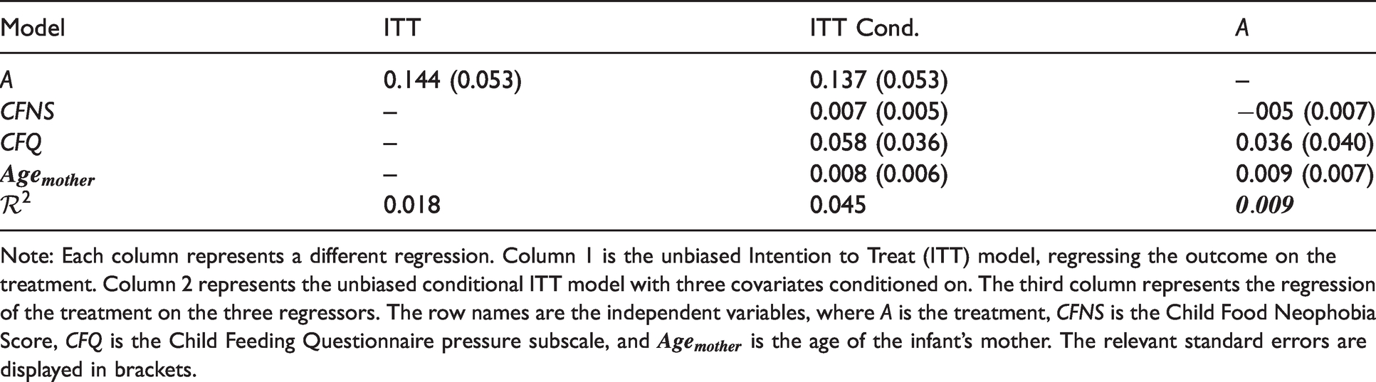
Our foundation is the unbiased ITT effect from the RCT data regressing the treatment on the outcome ( $Y\sim A$ ) shown in the first column of Table 1.

Table 1.

Clinical data regression table.

Model	ITT	ITT Cond.	A
A	0.144 (0.053)	0.137 (0.053)	–
CFNS	–	0.007 (0.005)	−005 (0.007)
CFQ	–	0.058 (0.036)	0.036 (0.040)
$\mathit{Ag}{\mathit{e}}_{\mathit{mother}}$	–	0.008 (0.006)	0.009 (0.007)
${\mathcal{R}}^2$	0.018	0.045	$\mathit{0}.\mathit{009}$

Note: Each column represents a different regression. Column 1 is the unbiased Intention to Treat (ITT) model, regressing the outcome on the treatment. Column 2 represents the unbiased conditional ITT model with three covariates conditioned on. The third column represents the regression of the treatment on the three regressors. The row names are the independent variables, where A is the treatment, CFNS is the Child Food Neophobia Score, CFQ is the Child Feeding Questionnaire pressure subscale, and $\mathit{Ag}{\mathit{e}}_{\mathit{mother}}$ is the age of the infant’s mother. The relevant standard errors are displayed in brackets.

In column 1 of Table 1, we see that the ITT estimate is 0.14. As this is an RCT, we do not expect baseline covariates [Child Food Neophobia Score ( CFNS ), Child Feeding Questionnaire ( CFQ ) subscale pressure, and Age of mother ( $\mathit{Ag}{\mathit{e}}_{\mathit{mother}}$ )] to be associated with exposure. We thus assume that the experimental data are generated from the causal DAG in Figure 7(a), where X represents the matrix of all three covariates ( CFNS , CFQ , and $\mathit{Ag}{\mathit{e}}_{\mathit{mother}}$ ) after they have been individually standardized to have mean 0 and variance 1. To verify that these variables are not bias amplifiers, that is explain only a negligible proportion of the treatment variance, we also present the results of the regression of the treatment on the three covariates in column 3 in Table 1. We can see that jointly and individually the three covariates explain very little of the variance in the treatment, ${\mathcal{R}}^2=0.009$ . This should be expected in a truly randomized experiment set-up since proper randomization breaks the causal association from the covariates to the treatment. Since these covariates do not cause A and we have assumed that the ITT estimator is unbiased, when we estimate $\mathit{Y}\sim \mathit{A}+\mathit{CFN}{\mathit{S}}_{\mathit{score}}+\mathit{CF}{\mathit{Q}}_{\mathit{pressure}}+\mathit{Ag}{\mathit{e}}_{\mathit{mother}}$ the expectation and probability limit of $\widehat{{\beta }_a}$ remains unchanged regardless of the strength of association between the covariates and the outcome. However, actual results may vary due to final sample variation. In our RCT data, the unadjusted model estimates a treatment effect of 0.144 and the adjusted model estimates 0.137. Since simulation experiments performed in section 6.2 all condition on covariates, we consider the covariate adjusted results from the RCT as the gold standard for determining bias due to unmeasured confounding in our simulated data.

Figure 7.

Causal diagrams. (a) DAG representing the original experiment data. (b) DAG with the modified data (see Appendix A.11 for details). (c) represents intervening on the causal DAG in (b) by changing the strength of the edge $\tilde{\mathit{X}}\to \mathit{A}$ without holding the latent treatment variance ${\mathit{A}}^{*}$ constant. The edges which have been modified inadvertently are shown as squiggly arrows. Parameters which have been changed are shown in red. (d) The intervention on the edge $\tilde{\mathit{X}}\to \mathit{A}$ while holding the latent variance constant.

Figure 8.

Here we compare three estimators for β_a from the structural equations in equations (22), (23), and (24). In red, the results of the unbiased and infeasible estimator are shown, centered at the true value ${\beta }_a=0.137$ (shown by the vertical black line). In green, the replications for the naive estimator ( ${\widehat{\beta }}_a^{\mathit{naive}}$ ) is shown and in blue the replications for the conditional estimator ( ${\widehat{\beta }}^{|\tilde{X}}$ ) is shown. Simulation details: Bootstrap replications = 10,000. ${\beta }_a=0.137,{\beta }_u=0.15,{\mathit{\beta }}_{\tilde{\mathit{x}}}=(0.10,-0.15,-0.10),\mathit{COV}(\mathit{A},\mathit{U})$  = 0.25, $\mathit{COV}\left(\mathit{A},\tilde{\mathit{X}}\right)=\left(0.22,0.15,0.13\right)$ .

Figure 9.

Control treatment estimators. Black line represents the true underlying parameter ${\beta }_a=.1377$ . N = 10,000 simulation replications.

6.2 Biased model simulations

Our objective is to simulate data according to the DAG in Figure 7(b). To produce the simulations, we took 10,000 bootstrap replications of the original outcome, treatment and covariates. From each bootstrap sample of the treatment, ${\mathit{A}}_{\mathit{bootstrap}}$ , of size n = 294 we simulated the latent variable ${\mathit{A}}^{*}$ using the procedure outlined in the Appendix (section A.11). Next, conditional on the drawn latent samples of ${\mathit{A}}^{*}$ and the bootstrapped covariates, we drew samples for the unmeasured confounding, U , and bias amplifying variable, BAV . The modified random control variables, $\tilde{\mathit{X}}=\frac{\mathit{X}}{\sigma \prime }+\mathit{BAV}$ , were produced by adding the bias amplifying variables to a scaled version of the original control variables. Linear combinations of the unmeasured confounding and modified covariates were then added with reasonable values to the outcome such that the following DAG and equations hold (see simulation results).

$$\tilde{\mathit{Y}}={\alpha }_y+\mathit{A}{\beta }_a+\tilde{\mathit{X}}{\beta }_{\tilde{x}}+\mathit{U}{\beta }_u+{ϵ}_{\mathit{1}}$$

(22)

$${\mathit{A}}^{*}={\alpha }_a+\mathit{U}{\gamma }_u+\tilde{\mathit{X}}{\gamma }_{\tilde{X}}+{ϵ}_{\mathit{2}}$$

(23)

$$\mathit{A}=1\{{\mathit{A}}^{*}>\mathit{0}\}$$

(24)

In section 6.1 we showed that the true treatment effect was 0.137 conditional on the covariates X . In the bootstrap simulation pictured below, the unbiased model conditional on both the modified covariates, $\tilde{\mathit{X}}$ , and the unmeasured confounding U is 0.136 as expected. The naive model estimator had an average estimate of 0.234 in the simulations and thus an absolute estimated bias of 0.097, or a relative bias of 1.8 standard deviations ( $\frac{0.234-0.137}{0.053}$ ) with respect to the unbiased estimate in section (6.1).

When we further condition on the modified covariates, the absolute bias ( $E[|{\widehat{\beta }}_a^{|\tilde{x}}-0.137|]$ ) more than doubles to 0.225, and the relative bias increases to 4.3 standard deviations ( $\frac{0.36-0.137}{0.053}$ ) with respect to the unbiased estimate in section 6.1. The simulations confirm that bias amplification can be significant even when constrained to problems of realistic variance. Further, we see that bias amplification is potentially a problem for binary outcomes. This underscores the theoretical points made in sections (3) and (4) where we showed that the phenomenon behind bias amplification does not require specific distributional assumptions of the variables in the model.

More importantly, by combining the methodology outline in the appendix (see Appendix A.11) to simulate measured confounding using real data and the principles for simulating systems of equations in section 5, we can produce realistic and complete simulations of parameter spaces which match the underlying characteristics of the data. Investigators who choose covariates based on the assumption of no unmeasured confounding can now evaluate the amount of bias amplification that would occur if this assumption does not hold.

Finally, in the Appendix (section A.12) we consider an example of a causal simulation experiment with a binary treatment variable under the DAG in Figure 7(b) and structural equations (22) to (24). The experiment involves modifying the strength of the edge $\widetilde{{\mathit{X}}_{\mathit{1}}}\to \mathit{A}$ and evaluating the impact on the naive and conditional estimators. With binary treatment ( A ), we show that if we fail to hold the variance of the latent treatment ( ${\mathit{A}}^{*}$ ) constant and increase ${\gamma }_{\widetilde{x_1}}$ , then it is possible to decrease the amount of observed treatment variance ( ${\sigma }_a^2$ ) explained by $\widetilde{{\mathit{X}}_{\mathit{1}}}$ . Further, the increased treatment variance also decreases the strength of the edge $\mathit{U}\to \mathit{A}$ . As a result of performing the causal simulation experiment improperly, it appears as though that varying the strength of the potential amplifiers has a negligible or negative impact on the resulting bias amplification. The improper and proper approaches to intervention are shown in Figure 7(c) and (d), respectively and the results from these simulations are visualized in Figure 10 of the Appendix section A.12. This of course leads to improper inferences regarding the relative merits of the naive and conditional estimators as well. This highlights once again the importance of comparing simulations with comparable properties and ensuring that when we intervene on the edges of our causal diagram that we are not inadvertently varying the edges we mean to keep fixed. Just as in the experimental context, our simulation results become muddled or meaningless if we are not evaluating well-articulated counterfactuals.

Figure 10.

The vertical lines represent the means from the control experiment: red representing the mean of unbiased control estimator, green the mean of the naive estimator, and blue the mean of the amplified estimator.

7 Discussion

Causal model selection techniques have largely been developed under the assumption that a sufficient set of variables is available to create ignorability. When a sufficient set is not available or when a causal variable selection technique does not correctly identify the sufficient set, we are at risk of bias amplification. In the first simulation in section 1, we showed that even under mild perturbations of the usual assumptions, conditioning on a set of jointly strong proxy variables for A in OLS led to a very biased estimator (0.73 standard deviations on average). Further, most current causal variable selection techniques are likely to include this set of variables since they are significant predictors of the outcome and the treatment as well as variables which cause large changes in estimates when included sequentially.

Under threat of bias amplification, treatment-oriented selection techniques for regression analyses using continuous exposure regimes should be used cautiously unless one has strong priors that a sufficient set is available and likely to be identified. We showed in section 3 that it is precisely the amount of variance in the treatment explained by the observables in our model which is responsible for bias amplification. Similarly, we can see that a significant change in estimate is not sufficient to suggest that overall bias is decreasing since this could be the result of further bias amplification.

These results call for new techniques to be developed for observational studies which can accommodate unmeasured confounding to help researchers choose reasonable and least-biased methods. We suggest to first identify the most plausible causal DAG. From the DAG and basic structural equation assumptions, an expression for asymptotic bias can often be derived. Further, we suggest to estimate the always-identifiable amplification term in observational settings and to assess the risk of bias amplification. With a measure for amplification and a limiting bias expression, a sensitivity analyses can be performed. One reasonable sensitivity analysis approach would be to estimate the amount of unmeasured confounding required in the spirit of E-values ⁷ to determine the strength of confounding associations required to “explain away the treatment effect” ⁷ and to make principled inferences from the data. This would require, as we have shown, properly simulating the unmeasured confounder so that (1) the properties of the original data are respected and (2) other competing effects, i.e. edges of the DAG, are not inadvertently altered. In such a set-up, large effects when the controls jointly explain little of the treatment variance lend credibility to results as being robust to unmeasured confounding, particularly in cases when suitable priors can be placed on the variables along the unmeasured confounding pathway. Alternatively, one could follow the approach of Carnegie et al. ⁸ and use the underlying structural equations and the data to generate candidate values of the unmeasured confounding. As we showed in section 5, it is important that any such simulation method take into account the asymmetry of bias amplification with respect to the weight of the edge $\mathit{U}\to \mathit{A}$ and $\mathit{U}\to \mathit{Y}$ .

Ultimately, simulation experiments must aim to produce data from which we can draw causal conclusions to questions about estimators or functions. This means having well-defined interventions on the edges of the causal graphs and holding the other edges constant. In linear systems of equations, this requires keeping the moments of the variables, in particular variance, fixed when modifying the weight of the DAG’s edges. If we allow the treatment variance to vary incidentally as we increase confounding effects, the intervention arm of our simulations will no longer match the target observational study in the control arm. As a further consequence, the additional variance in the exposure may absorb much of the amplifying effect. This leads to systematic underestimation of bias amplification and may be an explanation for why the threat of bias amplification has not been appreciated as a concern for applied researchers. ¹⁵ Fixing the variance of the variables has the additional benefit of defining the feasible parameter space. By constraining the underlying parameters by the implied variance equations, it is computationally and conceptually easier to simulate the entire range of plausible treatment effects and biases. This leads to more representative simulations and more principled inferences.

Supplemental Material

sj-zip-1-smm-10.1177_0962280221995963 - Supplemental material for Causal simulation experiments: Lessons from bias amplification

Supplemental material, sj-zip-1-smm-10.1177_0962280221995963 for Causal simulation experiments: Lessons from bias amplification by Tyrel Stokes, Russell Steele and Ian Shrier in Statistical Methods in Medical Research