
Abstract
Competing risks models can involve more than one time scale. A relevant example is the study of mortality after a cancer diagnosis, where time since diagnosis but also age may jointly determine the hazards of death due to different causes. Multiple time scales have rarely been explored in the context of competing events. Here, we propose a model in which the cause-specific hazards vary smoothly over two times scales. It is estimated by two-dimensional
Keywords
Introduction
Competing risks describe the situation where individuals are at risk of experiencing one of several types of events. 1 The prototype of a competing risks model is the study of cause-specific mortality. Such models are used in clinical studies of cancer to analyse mortality from cancer as well as mortality due to other causes as competing events.
The building blocks in a competing risks analysis are the cause-specific hazards (CSHs). They are defined as the instantaneous risk of experiencing an event of a specific type at time
Time is a key quantity in any survival analysis, and it can be recorded on several time scales. For example, after a cancer diagnosis, the risk of death may be studied over time since diagnosis, over age, which is time since birth, or over time since treatment. All time scales progress at the same speed and differ only in their origin. However, each time scale is a proxy for a specific mechanism linked to the event of interest. 2 In the study of mortality after a cancer diagnosis, time since diagnosis measures the cumulative adverse effect of the cancer. Additionally, as individuals age, they become more frail and their capacity of resisting comorbidity deteriorates.
Usually, CSHs are defined for the same single time scale, and little research has been done on how to handle multiple time scales in competing risks models. Existing studies focus on the choice of the time scale to use when modeling competing causes of deaths after a cancer diagnosis. Cancer mortality is clearly a function of time since diagnosis, while other causes of death are more naturally modeled over age. Whenever the CSHs of death for other causes are solely modeled over the time since diagnosis, bias may be introduced in the estimates of the cumulative incidences for cancer mortality. 3 Lee et al. 4 propose a model where two competing causes are modeled on two different time scales and then combined under one of the two scales to estimate the cumulative incidence functions.
Carollo et al.
5
introduced a model for a single event in which the hazard varies smoothly over two time scales simultaneously and is estimated by tensor products of
This study is motivated by the analysis of mortality after a breast cancer diagnosis. Breast cancer is the most common cancer diagnosed in women worldwide, 7 and the risk of being diagnosed with it increases over age, but varies by race and ethnic group, 8 with peaks of diagnosis after age 60 for white women and in the late 40s for non-white women. Survival probabilities after a breast cancer diagnosis are generally very high, with more than 80% of women with breast cancer being alive 10 years after diagnosis, 9 leading to many women living with a history of breast cancer for many years. Several studies have shown that breast cancer survivors are at higher risk of dying from cardiovascular disease (CVD),10–12 and there is evidence that this increased risk appears among survivors of breast cancer several years after diagnosis. 11 Increased CVD mortality rates among breast cancer survivors appear to be likely linked to adverse effects of therapy and to common risk factors. 12
Mortality rates of women with breast cancer depend on age, race and cancer subtypes,13,14 however, the relationship between time since diagnosis, age, age at diagnosis and mortality is not yet clear. Most studies of women with breast cancer find that breast cancer mortality increases after age 70 so that older women are at higher risk of dying because of the cancer.13,15,16 However, older women with breast cancer often die of causes other than cancer, with CVDs being the most common cause of non-cancer death. 12 Other studies have found that younger ages at diagnosis of breast cancer are associated with higher overall mortality14,17 and that women diagnosed before age 35 had higher risk of death because of cancer than older women. 18 Although most studies acknowledge the presence of several time scales, they do not account for them explicitly. For example, age at diagnosis is often grouped in broad and arbitrarily-cut categories, and interaction with time since diagnosis is often neglected. Shedding light on the way mortality rates of breast cancer vary with these two time scales, while properly accounting for competing causes, is both of empirical and of methodological relevance.
We analyse mortality data of women with breast cancer from the Surveillance, Epidemiology and End Results (SEER) registers 19 by time since cancer diagnosis and age. We focus on postmenopausal women (age at diagnosis 50 and older) and distinguish between deaths due to breast cancer and all other causes of death. In the SEER data, age at diagnosis is recorded in single years of age up to age 89 and one last open-ended interval for all individuals older than 89 (age at diagnosis 90+). Such grouping is common in data on disease incidence and/or mortality, usually to prevent identification of the patients or to provide a condensed depiction of the data. In this paper we employ the two-dimensional penalised composite link model (PCLM) 20 to ungroup the final age interval.
The remainder of this article is structured as follows: in Section 2 we first set the notation for the CSHs with two time scales and review the estimation procedure. Then we introduce calculation of cumulative CSHs, overall survival probabilities and finally cumulative incidence functions with two time scales, together with their standard errors. Section 3 is dedicated to the motivating example. A discussion concludes the paper.
A competing risks model with two time scales
Consider individuals that are diagnosed with cancer. Once a patient is diagnosed with the disease, he or she is at risk of dying from cancer (event of interest) or because of causes other than cancer (competing event). The risk of dying from cancer actually sets in at disease onset, however, since this onset is rarely known, time since diagnosis mainly is used as duration of the disease and we will also follow this practice.
For both competing events two time scales are relevant: the first is the age of the individual, which we indicate with
We consider two competing events: death from breast cancer (

The two time scales differ in their origin, so in the case of cancer patients
The same information can also be portrayed in the

From the CSHs
We will model (and estimate) the CSHs
The
Each individual
The contribution of an individual’s at-risk time per bin is, again, only in those cells where the first index
The

Because of the same-sized bins, event counts and at-risk times are on a regular grid and are naturally arranged as

To obtain smooth CSH surfaces we model the log-hazards
The tensor products are formed from two marginal

The numbers of basis functions

The objective function to be minimised is the sum of the Poisson deviance resulting from (4) and the above penalty (6)


The parameters


The calculations required in (8) can be done very efficiently by employing generalised linear array methods,
27
which is possible due to the regular grid of bins underlying
Once the estimated coefficients


Despite the popularity of penalised splines in practical applications, the derivation of their asymptotic properties had been lagging somewhat behind. Building on earlier work,
28
Xiao
29
presents
To obtain the overall survival function and the two cause-specific cumulative incidence functions, we first have to obtain the cumulative CSHs. In the model with two time scales this can be done in either of the two specifications, see equation (2):

The overall survival function correspondingly is

Finally, the two cumulative incidence functions (CIFs) are
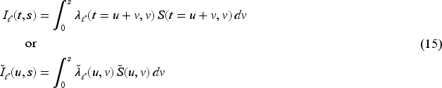
Integration in (13) and (15) is over one dimension only and we determine all integrals by numerical quadrature. Since we can evaluate the estimated CSHs on an arbitrarily fine grid, see (11), approximation errors will be minimal, even with a simple rectangle rule, as long as we choose a narrow enough grid width


The variance-covariance matrix of the coefficients

The standard error of the linear predictor


The standard errors for the cumulative incidence functions (CIFs) are obtained via nonparametric bootstrap. To corroborate the sampling distribution of the CIFs, we performed a simulation study that is presented in the Supplementary Material. Based on the results, confidence intervals for the CIFs were determined as Normal-based intervals with variances obtained from the empirical variances of the bootstrap estimates. Details about the bootstrap implementation for the SEER data will be discussed in Section 3.3.
The SEER data
The Surveillance, Epidemiology and End Results (SEER) program from the National Cancer Institute collects and publishes data on cancer incidence and survival covering about 48% of the population of the USA. 31 In this study we use data from the incidence SEER-17 database (November 2022 submission 32 ), that includes all cancer diagnoses up to 2020. We accessed the registers on 09/08/2023 and used the case listing functionality of SEER*Stat 33 to extract all cases of malignant breast cancer (primary site codes C50.0-C50.9) diagnosed to women between 2010 and 2015, with maximum follow-up to the end of 2020.
We focus on postmenopausal women and hence selected only women who were at least 50 years old when the cancer was diagnosed. Year of diagnosis was restricted to 2010–2015 to limit potential period effects, such as improvements in diagnosis and treatment efficacy that may affect survival probabilities. The potential maximum length of follow-up was several years for all women in the sample (although of different length, depending on the specific year of diagnosis).
Only individuals for whom the cancer was the first malignant tumor ever recorded in the SEER registry were included in the analysis. Furthermore, only cases for which the cancer was confirmed microscopically or by a positive test/marker study were included, while cases where the cancer was detected only by autopsy or only reported on the death certificate were not considered.
Mortality of breast cancer patients is known to depend on race/ethnicity,
34
independent of socioeconomic factors. SEER provides a variable that combines information on race and ethnicity and we distinguish between white women, black women and women of race/ethnicity other than white or black in our analysis. Also the cancer sub-type influences the survival chances,13,14 and the sub-types are categorised according to their hormone receptor status (HR+ or HR-) and to the status of the human epidermal growth factor 2 receptor (HER2+ or HER2
Cases for which no information on the cancer sub-type was available (7.8%) or where race/ethnicity information was unknown (0.4%) were not included in the analysis. SEER also provides information on whether chemotherapy was performed, but does not distinguish between cases where chemotherapy was not given and those where this information is missing. The final size of the dataset is 202,242 women. Table 1 gives a summary breakdown by race/ethnicity, cancer sub-type and chemotherapy status.
Sample size in each group identified by race/ethnicity, breast cancer subtype and chemotherapy status.
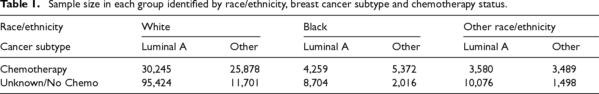
Sample size in each group identified by race/ethnicity, breast cancer subtype and chemotherapy status.
The key variables for our analysis are age at diagnosis, time since diagnosis, vital status at the end of the follow-up and, in case of death, whether death was attributable to the cancer or to any other cause of death. Time since diagnosis is available in the registry as survival months, that is the number of months from diagnosis to either death or right-censoring.
In the raw data, end of follow-up is fixed at the 31st of December 2020. However, since the COVID-19 pandemic in 2020 likely had a noticeable impact on cancer patients, we decided to limit the follow-up in our analyses to the end of 2019. For individuals who died before the end of 2019 no changes were required. For those individuals who were alive at the end of 2020 we subtracted 12 months of survival time and they were still right-censored at the end of 2019. Finally, individuals that died sometime in 2020 were right-censored at the end of 2019 and their survival times adjusted by 6 months, assuming that deaths occurred approximately 6 months into 2020, as is standard practice when the exact month of last follow-up is not available (see Supplementary Figure 1 for a graphical representation of this correction).
The different combinations of race/ethnicity, cancer sub-type and chemotherapy indicator define 12 groups of interest for our analysis. The sizes of the subgroups allow separate analyses so we estimate all models separately and compare the results among different groups. In the following we will present a subset of the analyses and refer to the supplementary material for more results.
Age at diagnosis is provided in the SEER registry as single years of age, up to age 89, and a last open-ended interval 90+. The distribution of age at diagnosis is shown in Figure 1, for the whole sample. Two features are clearly visible: first, the grouping of ages at diagnosis greater or equal to 90 (depicted as
The hazard model with two time scales that was introduced in Section 2.1 employs data that are binned in relatively narrow intervals of same size, resulting in data on a regular grid. The gridded structure allows efficient computations by using GLAM algorithms. To preserve this data structure, we will disaggregate the final age-group using the penalised composite link model (PCLM), the details can be found in Appendix A.1. Of the twelve subgroups (see Table 1) only eleven had observations with diagnoses made at age 90 or older, so the PCLM had only been applied in those subgroups. (Time since diagnosis is given in months for all individuals, also for those in this last age-interval, so only one time dimension is affected by coarse grouping.)
Before we ungroup the ages at diagnosis in the interval
The cause-specific event counts, and consequently the number of individuals at risk, for ages at diagnosis in the final wider interval are ungrouped using the PCLM as described in Appendix A.1 and the model specification is the same for all groups. The marginal
Figure 2 illustrates this approach for white women with luminal A subtype and no chemotherapy. The raw counts of breast cancer deaths are plotted in the left panel, the last age-interval is 10 years wide and corresponds to ages
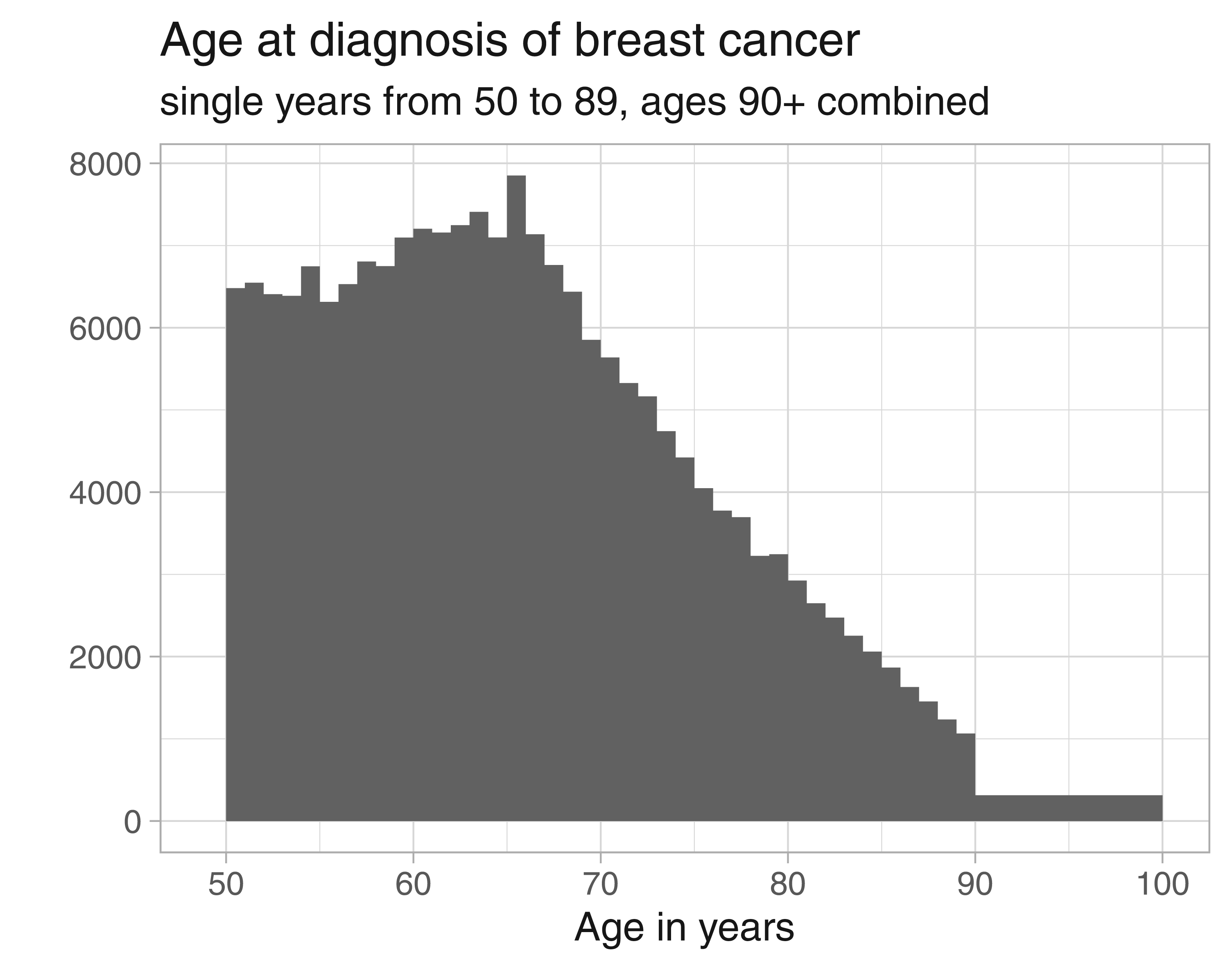
Distribution of age at diagnosis of breast cancer from the SEER data.
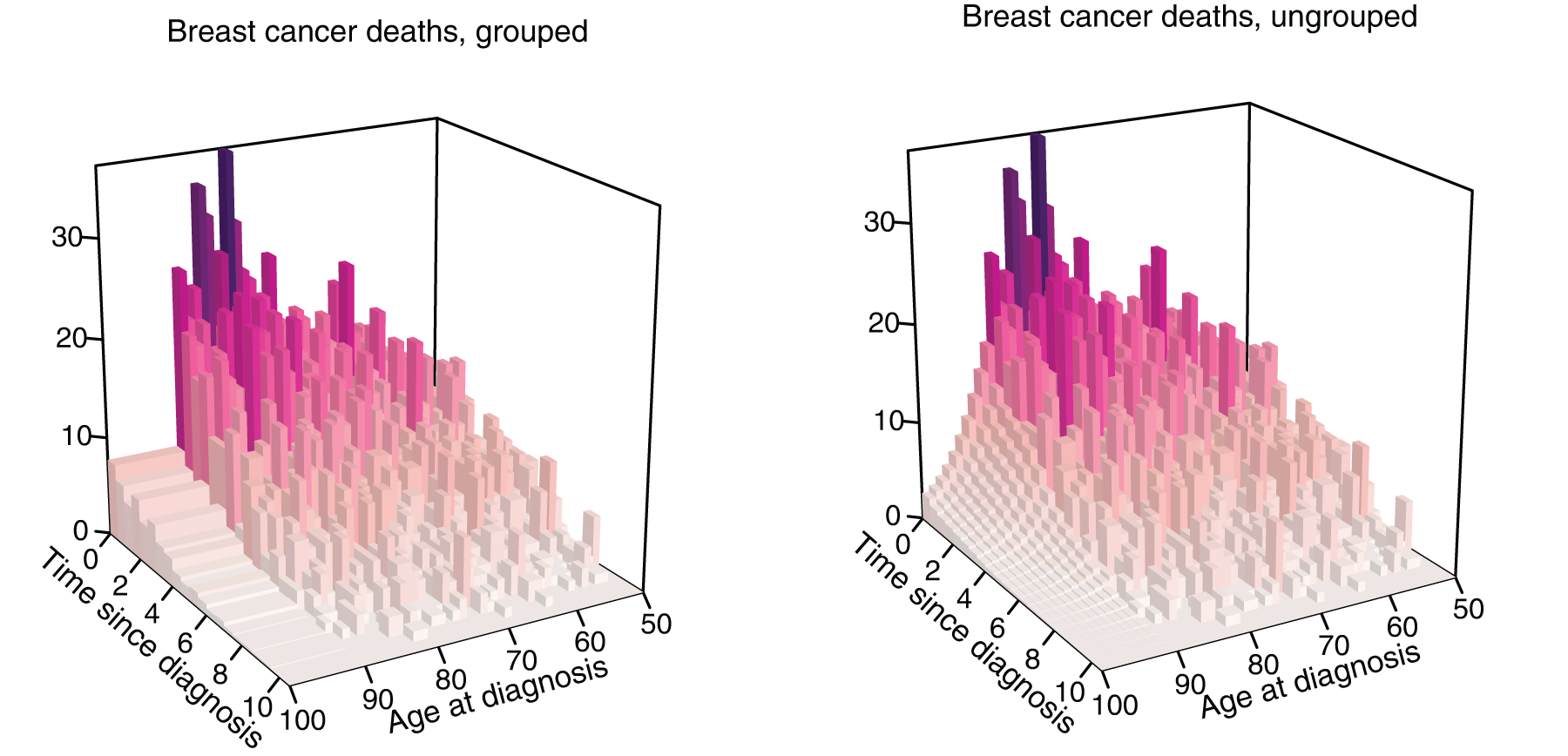
(Left) Histogram of deaths due to breast cancer over age at diagnosis (with ages
After having obtained estimates for the ungrouped event counts and exposure times, we replace the grouped data in
To illustrate the approach we present here the results for white women diagnosed with breast cancer of type other than Luminal A, both for patients who received chemotherapy and who did not. The distribution of the ages at diagnosis is given in Figure 3. Noticeable grouping of ages 90+ is discernible for women that received no chemotherapy.
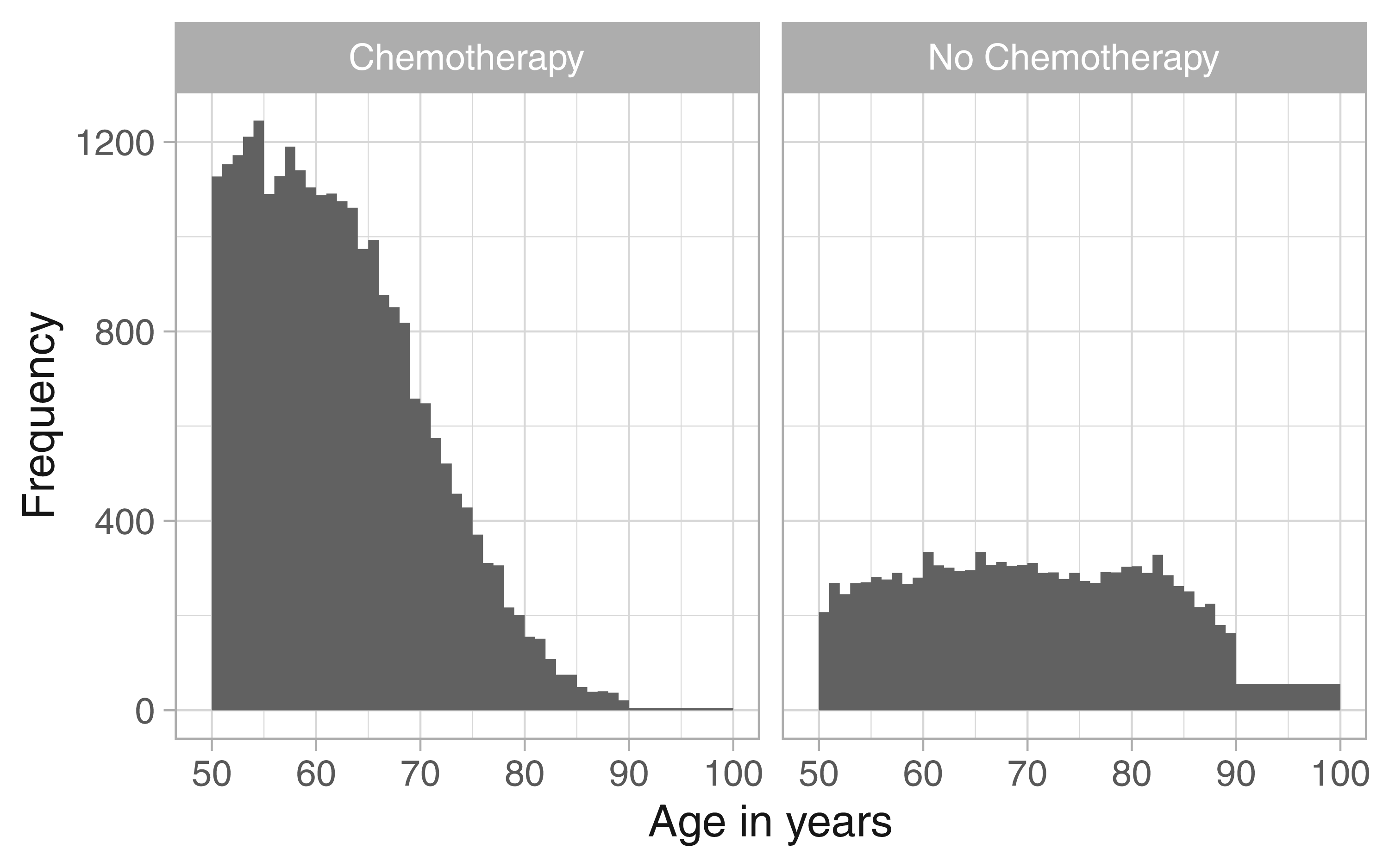
White women with cancer type other than Luminal A, age at diagnosis.
The matrices of event counts
Table 2 summarises the optimal smoothing parameters and the resulting effective dimensions for the two groups and the two causes of death, respectively. The estimated CSHs, on log10-scale, are shown in Figure 4.
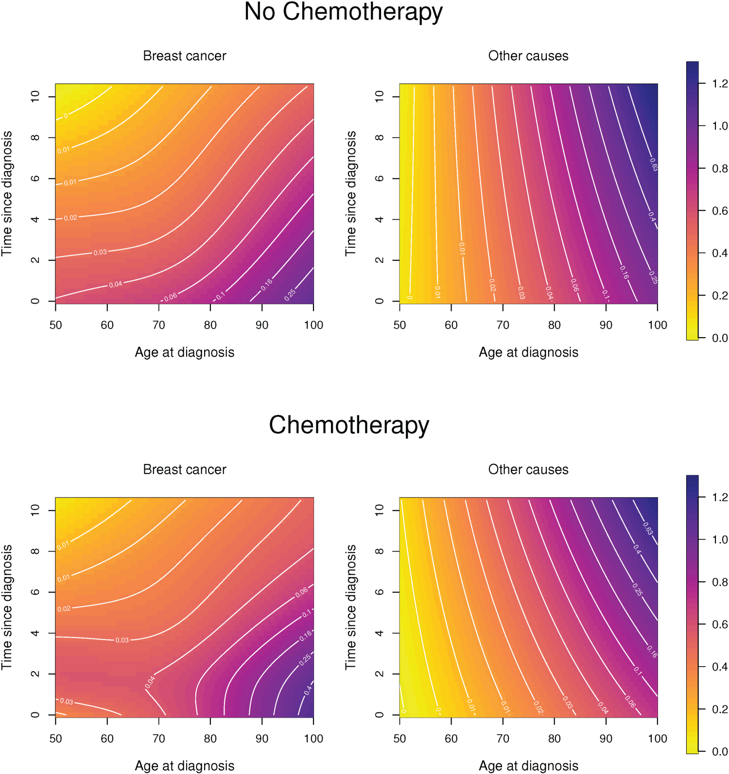
Cause-specific hazards for white women, other cancer types (non-Luminal A) who received chemotherapy (bottom row) and who did not (top row). Effective dimensions are given in Table 2.
White women with other subtypes: optimal smoothing parameters (minimal BIC) and resulting effective dimensions (ED) for cause-specific hazards.
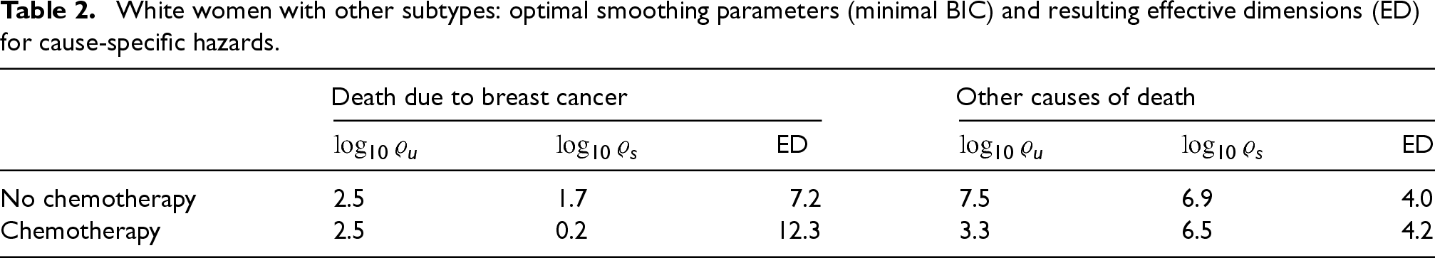
For women who did not receive chemotherapy the hazard of dying of breast cancer declines with time since diagnosis and it is generally higher if it was diagnosed at a higher age. If women did receive chemotherapy then, for age at diagnosis up to about age 75, the CSH for death due to breast cancer first increases and peaks about two years after diagnosis and declines thereafter. The different complexity of the hazard patterns is also reflected in the effective dimensions of the estimated hazard surfaces. The hazard of dying from other causes is, for both treatment groups, much smoother and reveals the well known exponential increase (Gompertz hazard) for ages 50+, however, the hazard level is lower for patients receiving chemotherapy but the increase in mortality over time is stronger for them.
The penalty allows to extend the estimated hazards into areas that are not supported by data. For example, in the specific application presented here, we know that for women who received chemotherapy and were diagnosed between age 90 and 100 the longest observed time since diagnosis was
It is already evident from Figure 4 that application of chemotherapy leads to a more complex change in the hazards than a proportional shift, but to investigate the differences further Figure 5 shows the hazard ratios of the two CSHs (for women who received chemotherapy relative to those who did not).
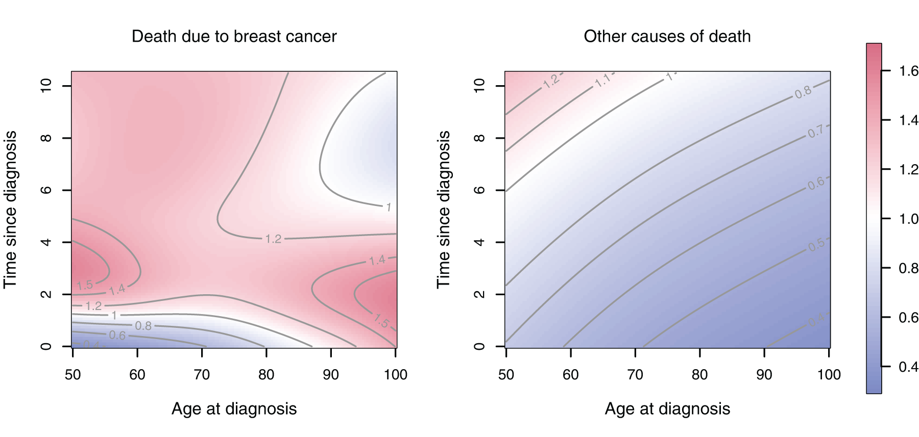
Ratio of the cause-specific hazards in Figure 4; chemotherapy versus no chemotherapy.
From the CSHs the overall survival function and the cumulative incidence functions can be derived, see Section 2.2. In Figure 6 we compare the cumulative incidence of death due to breast cancer and due to other causes for the treatment groups. The different lines correspond to different ages at diagnosis and result from transsecting the surfaces that are presented in Appendix A.2, Figure A.2 vertically. The overall survival probabilities for the two treatment groups can also be found there (Figure A.1).
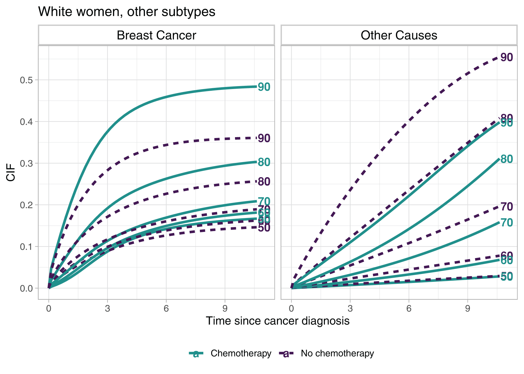
Cumulative incidence functions (CIFs) for selected ages at diagnosis over time since diagnosis. The complete surfaces of the CIFs can be found in Appendix A.2.
The gap of the cumulative incidence between the treatment groups widens for ages at diagnosis above 70, but while for breast cancer deaths the group that received chemotherapy shows higher values of the CIF, for the other causes of death the order reverses. For younger ages at diagnosis and time since diagnosis up to about 3 years the CIFs reflect the unimodal shape of the CSH in the chemotherapy group.
To obtain uncertainty estimates for the CIFs we perform a nonparametric bootstrap. We draw 500 bootstrap samples, and for each sample we first ungroup the last age interval. We fit the CSH models to the ungrouped data and finally we obtain estimates of the CIFs for each bootstrap sample.
We present the standard errors of the CIFs that were obtained as the empirical standard deviation over the 500 bootstrap samples in Figure A.3, comparing women with different therapy regimes. The two treatment groups are of quite different sizes (25,878 who received chemotherapy vs. 11,701 who did not) and this, together with the distribution of observations across the
Additional to the graphical displays of the estimates, which present the results in a comprehensive way but may be tedious to read, tabular summaries will be a useful supplement. The companion R-package also provides a function that allows to present estimates of overall survival and cumulative incidences, including bootstrap confidence intervals, in tabular form. An example is provided in Tables A.1 and A.2 in Appendix A.2.
In this article we present a method to estimate a competing risks model where the CSHs and hence also the derived quantities in the model vary over two time scales. The model is estimated by two-dimensional
The results of the proposed model are presented in several figures throughout the manuscript, and all graphs were produced using plotting functions in the R-package. While those figures provide compact illustrations of the estimates, numerical summaries may also be desirable. Hence the R-package also includes a function that produces tabular summaries of the estimated overall survival and cumulative incidence functions at specified values of
The GLAM approach rests upon data that are binned on a regular grid so that the array structure can be utilised in the computations. In practice we may encounter event times that are grouped in a wide interval for one or both time axes at the upper end of the time scale. The SEER data that we used in this paper provide such an example. To preserve the gridded structure of the data for estimating the CSHs we used the penalised composite link model to ungroup the final wide intervals. Again only smoothness of the underlying distributions is assumed and bivariate
The penalty allows to extend the estimates of the CSHs, and hence also the derived quantities, into areas not supported by data. The SEER analysis provided an example for women who were diagnosed with cancer at very high ages and for whom the hazards could be extrapolated beyond the longest life spans in the data. However, extrapolation should be done with caution, like with any other method. Examples of both unproblematic and more questionable extrapolation results are given in Carollo et al. 5
We analyse mortality after diagnosis of breast cancer and we distinguish between deaths due to breast cancer and all other causes of death. We consider two time scales, age and time since diagnosis. Extensions of the model to more than two competing events, analysed over the same time scales, is unproblematic. It is theoretically possible to consider more than two time scales, but it would imply greater computational complexity and is a topic for future research.
In the application we considered race/ethnicity, tumor type and chemotherapy status and analysed subgroups separately which, in this case, was feasible due to the large sample size of the SEER registers. This allowed, on the one hand, to use the PCLM for ungrouping as this model operates on aggregated count data. It also allowed to identify deviations from proportional hazards for the two treatment groups that were particularly pronounced for the hazard of death due to breast cancer. Nevertheless, for more covariates and less comprehensive data sets hazard regression models will be relevant tools for analysis, also for CSHs that vary along two time scales. For exactly observed event times proportional hazards regression has been developed already
5
and is also implemented in the R-package
Supplemental Material
sj-pdf-1-smm-10.1177_09622802251367443 - Supplemental material for Competing risks models with two time scales
Supplemental material, sj-pdf-1-smm-10.1177_09622802251367443 for Competing risks models with two time scales by Angela Carollo, Hein Putter, Paul HC Eilers and Jutta Gampe in Statistical Methods in Medical Research
Footnotes
Data availability statement
Declaration of conflicting interests
The authors declared no potential conflicts of interest with respect to the research, authorship and/or publication of this article.
Funding
The authors received no financial support for the research, authorship and/or publication of this article.
Supplemental material
Supplemental material for this article is available online.
Appendix A
References
Supplementary Material
Please find the following supplemental material available below.
For Open Access articles published under a Creative Commons License, all supplemental material carries the same license as the article it is associated with.
For non-Open Access articles published, all supplemental material carries a non-exclusive license, and permission requests for re-use of supplemental material or any part of supplemental material shall be sent directly to the copyright owner as specified in the copyright notice associated with the article.