On estimation of overall treatment effects in multiregional clinical trials under a discrete random effects model

Abstract

Multiregional clinical trials (MRCTs) have become a standard strategy for pharmaceutical product development worldwide. The heterogeneity of regional treatment effects is anticipated in an MRCT. For a two-group comparative study in an MRCT, patient assignments, including regional weights and treatment allocation ratios, are predetermined under the same protocol. In practice, the observed patient assignments at the final analysis stage are often not equal to the predetermined patient assignments, which may impact the accuracy of estimating the overall treatment effect and may lead to a biased estimator. In this study, we use a discrete random effects model (DREM) to account for the heterogeneous treatment effect across regions in an MRCT and propose a bias-adjusted estimator of the overall treatment effect through a naïve estimator conditioned on ancillary statistics based on the observed patient assignments at the final analysis stage in the trial. We also perform power analysis for the overall treatment effect and determine the overall sample size for the bias-adjusted estimator with the DREM. Results of simulation studies are given to illustrate applications of the proposed approach. Finally, we provide an example to demonstrate the implementation of the proposed approach.

1. Introduction

With the development of global pharmaceutical products, multiregional clinical trials (MRCTs) have become a standard strategy. In an MRCT, patients are recruited from multiple geographical regions under the same protocol. Ensuring the accuracy of effect estimates is crucial for demonstrating the clinical benefits of test drugs.

Traditionally, the same treatment effects are assumed for all participating regions in an MRCT. However, in reality the treatment effects show regional variations, which are often due to differences in race, diet, environment, culture, and medical practice among regions. Therefore, when regional heterogeneity is anticipated, the assumption that regional treatment effects are not identical would be more appropriate in the design of MRCTs.^1,2 To address this issue, Lan and Pinheiro ³ proposed the discrete random effects model (DREM) to account for heterogeneous treatment effects across regions. The DREM framework is applicable in practical situations. For example, Liu et al. ⁴ used the DREM with a continuous endpoint for the design and evaluation of MRCTs. Moreover, Lan et al. ⁵ extended the application of the DREM from a continuous endpoint to time-to-event and binary endpoints.

In a two-group comparative study of an MRCT, patients are recruited from each region according to regional weights and then randomly assigned to the two groups. During the design stage, the regional weights are predetermined based on the population size, market size, prevalence of disease, and cost-effectiveness. Under a common protocol, it is generally assumed that the same treatment allocation ratio is used for all participating regions during the design stage. However, at the final analysis stage, the observed patient assignments are often not the same as the predetermined ones. That is, the regional weights and treatment allocation ratios vary among regions. For instance, differences in the observed treatment allocation ratios across regions in practice may be due to patients lost to follow-up, dropout rate, drug side effects, or other reasons. Therefore, the accuracy of estimating the overall treatment effect may be compromised, resulting in a biased estimator. Ignoring the potential bias in an estimator may lead to overestimation or underestimation of the overall treatment effect.

To quantify the potential bias caused by the differences between the observed patient assignments and the predetermined ones, Tian et al. ⁶ used a conditional distribution, which enhances our understanding of the efficiency augmentation procedure, in the stratified analysis. Of note, a conditional distribution with reasonable auxiliary statistics can be more informative than an unconditional distribution.^7,8 In this article, we extend the approach of Tian et al. ⁶ to obtain a bias-adjusted estimator for the overall treatment effect. Furthermore, we conduct power analysis for the overall treatment effect and determine the overall sample size by adjusting for the potential impact caused by these differences.

The odds ratio (OR) is a common measure for the binary endpoint in two-group comparative studies. In this study, we adopt the OR as an example to illustrate our approach. Additionally, both the observed regional weights and the observed treatment allocation ratios are considered as auxiliary statistics.

We organize the rest of this article as follows. In Section 2, we introduce the DREM and propose to construct a bias-adjusted estimator for the overall treatment effect under the DREM. In Section 3, we describe the hypothesis for our proposed approach using the DREM, derive the power functions for the resulting test statistic and the naïve estimator, and determine the required sample sizes. In Section 4, we provide simulation studies that investigate the performance of the proposed approach. An example is illustrated in Section 5, and some concluding remarks are given in Section 6.

2. Adjusting the naïve estimator under the DREM

2.1. DREM with binary endpoints

To address the heterogeneous treatment effect across regions in an MRCT, the DREM was proposed by Lan and Pinheiro. ³ In this section, we present the application of the DREM to binary endpoints ⁵ by taking the OR as an example.

We consider the patient population to be partitioned into K disjointed clinical regions. The regional weight of region k is represented by $w_k,k=1,\dots ,K,$ with ${\sum }_{k=1}^K{w}_k=1,$ where $w_k$ is a parameter rather than a random variable. ³ In a randomized control trial, patients are randomly assigned to either the treatment group or the control group. Suppose that the patient-allocation ratio of the treatment group and the control group is $T:C$ and let $\pi =T/(T+C)$ , which represents the overall treatment allocation ratio. The treatment allocation ratio for region k is denoted as ${\pi }_k,k=1,\dots ,K,$ where ${\pi }_k$ is a parameter rather than a random variable. ³ Note that the overall treatment allocation ratio $\pi$ can be expressed as the weighted sum of ${\pi }_k$ , i.e., $\pi ={\sum }_{k=1}^K{w}_k{\pi }_k$ .

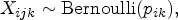
When the primary endpoint is binary, to compare the treatment effect in the treatment group and the control group, the overall treatment effect is estimated by the event rates of the two groups. The Bernoulli random variable $X_{ijk}$ is used to indicate whether the event occurs or not for the jth patient in the kth region for group $i=T,C.$ We assume that

$$X_{ijk}\sim \text{Bernoulli}(p_{ik}),$$

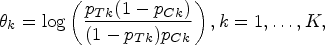
where $p_{ik}$ represents the true event rate of group i in the kth region. The regional treatment effect is defined as:

$${\theta }_k=\log \left(\frac{p_{Tk}(1-p_{Ck})}{(1-p_{Tk})p_{Ck}}\right),k=1,\dots ,K,$$

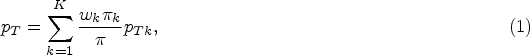
which is the log(OR) for the kth region. Let us now consider the overall treatment effect. It is important to note that the event rates for the treatment group overall and the control group overall are defined as follows:

$$\begin{array}{rl}{p}_T& =\sum _{k=1}^K\frac{w_k{\pi }_k}{\pi }{p}_{Tk},\end{array}$$

(1)

$$\begin{array}{rl}{p}_C& =\sum _{k=1}^K\frac{w_k(1-{\pi }_k)}{1-\pi }{p}_{Ck},\end{array}$$

(2)

where $w_k{\pi }_k/\pi$ and $w_k(1-{\pi }_k)/(1-\pi )$ are modified weights reflecting both the regional weight $w_k$ and the treatment allocation ratio ${\pi }_k$ . Thus, we can define the overall treatment effect as

$$\begin{array}{r}\theta =\log (OR)=\log \left(\frac{p_T(1-p_C)}{(1-p_T)p_C}\right).\end{array}$$

(3)

Assuming that a lower event rate represents a better outcome, a log(OR) of less than zero would favor the treatment group.

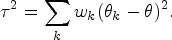
Under the DREM, the treatment effect for a randomly selected patient in the population is a random variable with the distribution defined by the possible values $\{{\theta }_1,{\theta }_2,\dots ,{\theta }_K\}$ and their respective probabilities $\{w_1,w_2,\dots ,w_K\}$ . The mean is $\theta$ and the between-region variance ( ${\tau }^2$ ) is expressed as

$${\tau }^2=\sum _k{w}_k({\theta }_k-\theta {)}^2.$$

To demonstrate how to calculate ${\tau }^2$ , we provide an example of an MRCT with three regions in Table 1. By considering $(w_1,w_2,w_3)=(0.35,0.35,0.30)$ and $({\pi }_1,{\pi }_2,{\pi }_3)=(0.5,0.5,0.5)$ , Table 1 exhibits the between-region variance ${\tau }^2$ for different event rates. As shown in the first row of Table 1, given $(p_{T1},p_{T2},p_{T3})=(0.50,0.60,0.60)$ for the treatment group and $(p_{C1},p_{C2},p_{C3})=(0.65,0.70,0.70)$ for the control group, we obtain $({\theta }_1,{\theta }_2,{\theta }_3)=(-0.62,-0.44,-0.44)$ , $\theta =-0.50$ , and ${\tau }^2=0.0071$ .

Table 1.

Between-region variance ${\tau }^2$ for event rates $p_{Tk}$ and $p_{Ck}$ , given $(w_1,w_2,w_3)=(0.35,0.35,0.30)$ and $({\pi }_1,{\pi }_2,{\pi }_3)=(0.5,0.5,0.5)$ .

$p_{T1}$	$p_{T2}$	$p_{T3}$	$p_{C1}$	$p_{C2}$	$p_{C3}$	${\tau }^2$
0.50	0.60	0.60	0.65	0.70	0.70	0.0071
0.55	0.60	0.65	0.70	0.75	0.80	0.0024
0.40	0.40	0.45	0.60	0.60	0.60	0.0088

When a patient from the population is randomly selected, the variance of his/her treatment effect should not only consider the between-region variance ${\tau }^2$ , but also take into account the within-region variance. For a patient from region k in group i, the within-region variance is the variance of $\text{Bernoulli}(p_{ik})$ , which is denoted as ${\sigma }_{ik}^2=p_{ik}(1-p_{ik})$ . As a result, we define the variance of the random variable $X_{ijk}$ as

$$\begin{array}{r}\text{Var}(X_{ijk})={\sigma }_{ik}^2+{\tau }^2.\end{array}$$

(4)

Let the sample size of region k be $N_k$ and the total sample size across all K regions be $N={\sum }_{k=1}^K{N}_k,k=1,\dots ,K$ . Within region k, let the sample size for group i be $N_{ik},i=T,C.$ If the sample size $N_{ik}$ is reasonably large, the event rate $p_{ik}$ can be adequately estimated by ${\hat{p}}_{ik}={\sum }_{j=1}^{N_{ik}}{X}_{ijk}/N_{ik}$ . The observed regional weight is ${\hat{w}}_k=N_k/N$ with ${\sum }_k{\hat{w}}_k=1$ , the observed treatment allocation ratio is ${\hat{\pi }}_k=N_{Tk}/N_k$ , in the kth region, and the observed overall treatment allocation ratio is $\overline{\pi }={\sum }_{k=1}^K{\hat{w}}_k{\hat{\pi }}_k$ . The event rates for the treatment group overall and the control group overall are estimated by ${\hat{p}}_T={\sum }_{k=1}^K({\hat{w}}_k{\hat{\pi }}_k/\overline{\pi }){\hat{p}}_{Tk}$ and ${\hat{p}}_C={\sum }_{k=1}^K({\hat{w}}_k(1-{\hat{\pi }}_k)/(1-\overline{\pi })){\hat{p}}_{Ck}$ , respectively. Therefore, according to Tian et al. ⁶ we can obtain the naïve estimator of the overall treatment effect as

$$\begin{array}{r}\hat{\theta }=\log \left(\frac{{\hat{p}}_T(1-{\hat{p}}_C)}{(1-{\hat{p}}_T){\hat{p}}_C}\right).\end{array}$$

(5)

The estimator of treatment effect for region k is ${\hat{\theta }}_k=\text{log}({\hat{p}}_{Tk}(1-{\hat{p}}_{Ck})/(1-{\hat{p}}_{Tk}){\hat{p}}_{Ck})$ , and the variance ${\tau }^2$ is estimated by ${\hat{\tau }}^2={\sum }_{k=1}^K{\hat{w}}_k{({\hat{\theta }}_k-\hat{\theta })}^2.$

2.2. Adjusting the naïve estimator

So far, we have defined the overall treatment effect $\theta$ (Eq. (3)) and have obtained the naïve estimator $\hat{\theta }$ (Eq. (5)). We will now discuss the potential bias of $\hat{\theta }$ and how to quantify it. As a common protocol is used in an MRCT, we generally assume that the overall treatment allocation ratio $\pi$ is applied across all K regions, meaning that $\pi ={\pi }_1=\dots ={\pi }_K$ . However, in practice, at the final analysis stage, the treatment allocation ratios ${\hat{\pi }}_k{}^{\mathrm{\prime }}s$ and the regional weights ${\hat{w}}_k{}^{\mathrm{\prime }}s$ may differ from those predetermined at the design stage. This reduces the accuracy of estimating the overall treatment effect. In this article, we take into account the gap between the design stage and the actual implementation results with the following assumptions:

(1)

the observed regional weights ${\hat{w}}_k{}^{\mathrm{\prime }}s$ are possibly different from the predetermined regional weights $w_k{}^{\mathrm{\prime }}s$ in the protocol, and

(2)

the observed treatment allocation ratios ${\hat{\pi }}_k{}^{\mathrm{\prime }}s$ are possibly different across regions.

Although efforts are made to enroll patients from each region to achieve predetermined regional weights $w_k{}^{\mathrm{\prime }}s$ and a predetermined treatment allocation ratio $\pi$ , they are often different in practice. We recognize this “real-world” challenge and attempt to fully understand its impact on the overall treatment effect. We anticipate that the observed naïve estimator $\hat{\theta }$ would not be equal to $\hat{\theta }$ based on the predetermined patient assignments.

One approach to empirically quantify the bias of $\hat{\theta }$ is to use conditional inference with ancillary statistics for $\theta$ .^6,9 There is a vast amount of literature on how to adjust the estimator based on baseline covariate information under unconditional inference.^10–13 In this study, we focus on the conditional distribution of $\hat{\theta }-\theta$ given appropriate ancillary statistics, as it is more informative than unconditional inference to study the stochastic behavior of $\hat{\theta }$ .^7,8 Here, both the observed regional weights $\{{\hat{w}}_k,k=1,\dots ,K\}$ and the observed treatment allocation ratios $\{{\hat{\pi }}_k,k=1,\dots ,K\}$ are ancillary statistics.

We consider the naïve estimator $\hat{\theta }$ to be generated through random sampling, but $\{({\hat{w}}_k,{\hat{\pi }}_k),k=1,\dots ,K\}$ of each sample would be the same as the observed patient assignment. We also assume random sampling of patients from each region and then their random assignment to one of two groups. Within the framework of the DREM, we extend the method proposed by Tian et al. ⁶ By the Central Limit Theorem, it can be readily shown that the conditional distribution of $(\hat{\theta }-\theta )|\{({\hat{w}}_k,w_k,{\hat{\pi }}_k,\overline{\pi }),k=1,\dots ,K\}$ is approximately normal, with the mean of

$$b_{\theta }=\frac{1}{(1-p_T)p_T}\sum _{k=1}^K{p}_{Tk}\left(\frac{{\hat{w}}_k{\hat{\pi }}_k}{\overline{\pi }}-w_k\right)-\frac{1}{(1-p_C)p_C}\sum _{k=1}^K{p}_{Ck}\left(\frac{{\hat{w}}_k(1-{\hat{\pi }}_k)}{1-\overline{\pi }}-w_k\right),$$

and the variance of

$$\begin{array}{r}{\sigma }_{\pi w}^2={\left(\frac{1}{(1-p_T)p_T}\right)}^2\sum _{k=1}^K{w_k}^{2}Var({\hat{p}}_{Tk})+{\left(\frac{1}{(1-p_C)p_C}\right)}^2\sum _{k=1}^K{w_k}^{2}Var({\hat{p}}_{Ck}).\end{array}$$

(6)

It is worth noting that the variance of ${\hat{p}}_{ik}$ accounts for both between-region and within-region variations. According to Eq. (4), the variance of ${\hat{p}}_{ik}$ can be derived as

$$\begin{array}{r}\text{Var}({\hat{p}}_{ik})=\frac{{\sigma }_{ik}^2+{\tau }^2}{N_{ik}},i=T,C.\end{array}$$

(7)

Next, let $p_i^{*}={\sum }_{k=1}^K{w}_k{\hat{p}}_{ik}$ be another estimator of $p_i$ (Eqs. (1) and (2)). Note that if ${\hat{w}}_k=w_k$ and ${\hat{\pi }}_k=\overline{\pi },k=1,\dots ,K$ , then the estimator ${\hat{p}}_i$ is equal to the estimator $p_i^{*}$ . Following Tian et al., ⁶ define $p_T^{*}={\sum }_{k=1}^K{w}_k{\hat{p}}_{Tk}$ and $p_C^{*}={\sum }_{k=1}^K{w}_k{\hat{p}}_{Ck}$ . Using the aforementioned notation, we construct an estimator of $b_{\theta }$ as

$${\hat{b}}_{\theta }=\frac{1}{(1-p_T^{*})p_T^{*}}\sum _{k=1}^K{\hat{p}}_{Tk}\left(\frac{{\hat{w}}_k{\hat{\pi }}_k}{\overline{\pi }}-w_k\right)-\frac{1}{(1-p_C^{*})p_C^{*}}\sum _{k=1}^K{\hat{p}}_{Ck}\left(\frac{{\hat{w}}_k(1-{\hat{\pi }}_k)}{1-\overline{\pi }}-w_k\right),$$

and an estimator of ${\sigma }_{\pi w}^2$ as

$${\hat{\sigma }}_{\pi w}^2={\left(\frac{1}{(1-p_T^{*})p_T^{*}}\right)}^2\sum _{k=1}^K{w_k}^2\frac{{\hat{\sigma }}_{Tk}^2+{\hat{\tau }}^2}{N_{Tk}}+{\left(\frac{1}{(1-p_C^{*})p_C^{*}}\right)}^2\sum _{k=1}^K{w_k}^2\frac{{\hat{\sigma }}_{Ck}^2+{\hat{\tau }}^2}{N_{Ck}},$$

where ${\hat{\sigma }}_{ik}^2={\hat{p}}_{ik}(1-{\hat{p}}_{ik}),i=T,C$ . By adjusting $\hat{\theta }$ directly, we can obtain

$$\begin{array}{r}{\hat{\theta }}_{\pi w}=\hat{\theta }-{\hat{b}}_{\theta }.\end{array}$$

(8)

The bias-adjusted estimator ${\hat{\theta }}_{\pi w}$ is the sum of $\hat{\theta }$ and a function of $({\hat{w}}_k,w_k,{\hat{\pi }}_k,\overline{\pi }),k=1,\dots ,K$ . Note that ${\hat{\theta }}_{\pi w}$ is a consistent estimator of $\theta$ . Moreover, the conditional distribution $({\hat{\theta }}_{\pi w}-\theta )|\{({\hat{w}}_k,w_k,{\hat{\pi }}_k,\overline{\pi }),k=1,\dots ,K\}$ under the null hypothesis is approximately normal with mean 0 and variance ${\sigma }_{\pi w}^2$ .

3. Power analysis and sample size determination under the DREM

3.1. Sample size calculation for the bias-adjusted estimator

The hypothesis test for the overall treatment effect under the DREM is

$H_0:\theta =0$ versus. $H_1:\theta <0.$

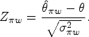
Here, if the overall treatment effect $\theta$ (Eq. (3)) is less than 0, it indicates that the treatment is effective, since we assumed that an OR of less than 1 is in favor of the treatment group (when the event rate represents death or disease recurrence, etc.). Utilizing the proposed estimator ${\hat{\theta }}_{\pi w}$ , the test statistic is given by

$$Z_{\pi w}=\frac{{\hat{\theta }}_{\pi w}-\theta }{\sqrt{{\sigma }_{\pi w}^2}}.$$

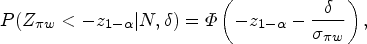
It is easily seen that the conditional distribution of the test statistic $Z_{\pi w}$ under the null hypothesis is approximately standard normal. The efficacy of the treatment group is claimed beneficial if the test statistic  $Z_{\pi w}<-z_{1-\alpha }$ , where $z_{1-\alpha }$ represents the $100(1-\alpha )\text{th}$ percentile of the standard normal distribution. Thus, the power function is

$$P(Z_{\pi w}<-z_{1-\alpha }|N,\delta )=\Phi \left(-z_{1-\alpha }-\frac{\delta }{{\sigma }_{\pi w}}\right),$$

where $\delta =\theta -0=\theta$ , $\Phi$ is the cumulative distribution function of the standard normal distribution, and $z_{1-\alpha }\approx 1.96$ if one-sided $\alpha =2.5\mathrm{\%}$ . In order to calculate the total required sample size N to detect $\delta <0$ , we converted the variance ${\sigma }_{\pi w}^2$ (Eq. (6) and Eq. (7)) into an expression involving N using $N_{Tk}=N{\hat{w}}_k{\hat{\pi }}_k$ and $N_{Ck}=N{\hat{w}}_k(1-{\hat{\pi }}_k)$ . It can be obtained that ${\sigma }_{\pi w}^2=B/N$ , where

$$\begin{array}{r}B={\left(\frac{1}{(1-p_T)p_T}\right)}^2\sum _{k=1}^K{w_k}^2\left(\frac{{\sigma }_{Tk}^2+{\tau }^2}{{\hat{w}}_k{\hat{\pi }}_k}\right)+{\left(\frac{1}{(1-p_C)p_C}\right)}^2\sum _{k=1}^K{w_k}^2\left(\frac{{\sigma }_{Tk}^2+{\tau }^2}{{\hat{w}}_k(1-{\hat{\pi }}_k)}\right).\end{array}$$

(9)

As shown in Eq. (9), B is the combination of regional variances, which include the variance of the Bernoulli random variable ${\sigma }_{ik}^2,i=T,C,$ between-region variance ${\tau }^2$ , observed regional weights $\{{\hat{w}}_k\}$ , observed treatment allocation ratio $\{{\hat{\pi }}_k\}$ , and predetermined regional weights $\{w_k\}$ . Given the significance level $\alpha$ and the power $1-\beta$ at the design stage, the total sample size required for ${\hat{\theta }}_{\pi w}$ is

$$\begin{array}{r}{N}_{\pi w}={\left(\frac{z_{1-\alpha }+z_{1-\beta }}{\delta }\right)}^{2}B.\end{array}$$

(10)

3.2. Sample size calculation for the naïve estimator

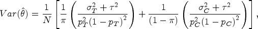
In this section, we introduce the distribution of the naïve estimator $\hat{\theta }$ and derive the required sample size. The estimator $\hat{\theta }$ follows an approximately normal distribution with the mean of $\theta$ and the variance of $\text{Var}(\hat{\theta })$ . To calculate the variance $\text{Var}(\hat{\theta })$ , let $g(p)=\text{log}(p/(1-p))$ , which is the log odds function of the event rate p. Then, through Taylor's expansion, $g(\hat{p})\approx g(p)+(\hat{p}-p)(1/(p(1-p)))$ . Taking the variance on both sides, we obtain

$$\begin{array}{r}\text{Var}(g(\hat{p}))\approx {\left(\frac{1}{p(1-p)}\right)}^2\text{Var}(\hat{p}).\end{array}$$

(11)

Under the DREM, substituting Eq. (7) into Eq. (11) and considering the log(OR) of the treatment and control groups, we obtain

$$Var(\hat{\theta })=\frac{1}{N}\left[\frac{1}{\pi }\left(\frac{{\sigma }_T^2+{\tau }^2}{p_T^2{(1-p_T)}^2}\right)+\frac{1}{(1-\pi )}\left(\frac{{\sigma }_C^2+{\tau }^2}{p_C^2{(1-p_C)}^2}\right)\right],$$

where ${\sigma }_i^2=p_i(1-p_i),i=T,C.$ Therefore, the test statistic for the naïve estimator $\hat{\theta }$ is given by $Z_{ne}=(\hat{\theta }-\theta )/\sqrt{\text{var}(\hat{\theta })}$ , and the required sample size for $\hat{\theta }$ is

$$\begin{array}{r}{N}_{ne}={\left(\frac{z_{1-\alpha }+z_{1-\beta }}{\delta }\right)}^2\left[\frac{1}{\pi }\left(\frac{{\sigma }_T^2+{\tau }^2}{p_T^2{(1-p_T)}^2}\right)+\frac{1}{(1-\pi )}\left(\frac{{\sigma }_C^2+{\tau }^2}{p_C^2{(1-p_C)}^2}\right)\right].\end{array}$$

(12)

We have thus derived the sample sizes $N_{\pi w}$ (Eq. (10)) and $N_{ne}$ (Eq. (12)) for ${\hat{\theta }}_{\pi w}$ and $\hat{\theta }$ , respectively.

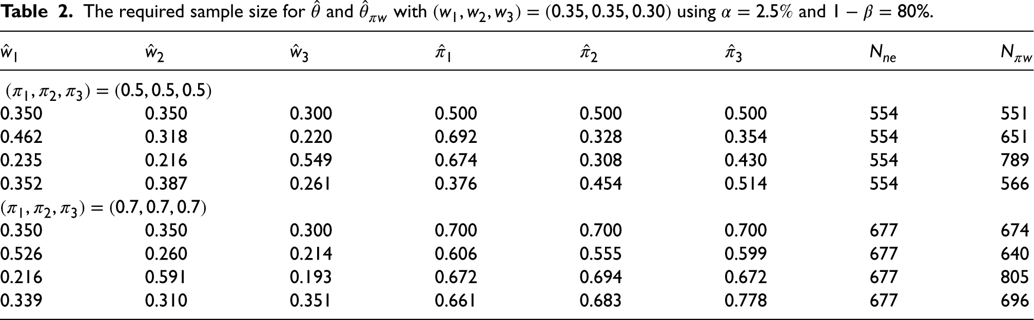
With $\alpha =2.5\mathrm{\%}$ , $\beta =20\mathrm{\%}$ , $(p_{T1},p_{T2},p_{T3})=(0.50,0.60,0.60)$ , $(p_{C1},p_{C2},p_{C3})=(0.65,0.70,0.70)$ , and $(w_1,w_2,w_3)=(0.35,0.35,0.30)$ , along with ${\tau }^2=0.0071$ , Table 2 shows the sample sizes $N_{ne}$ and $N_{\pi w}$ required for given observed patient assignments $({\hat{w}}_1,{\hat{w}}_2,{\hat{w}}_3,{\hat{\pi }}_1,{\hat{\pi }}_2,{\hat{\pi }}_3)$ . Although a treatment allocation of $T:C=1:1$ is common in an MRCT, there may be a higher proportion in the treatment arm in some clinical trials.^14,15 Therefore, we considered two cases: ${\pi }_k^{{}^{\mathrm{\prime }}}s=0.5$ and ${\pi }_k^{{}^{\mathrm{\prime }}}s=0.7$ , as shown in the top and bottom halves of Table 2, respectively. In both cases, the first row shows that the observed patient assignments were equal to the designed ones, i.e., ${\hat{w}}_k=w_k$ and ${\hat{\pi }}_k={\pi }_k$ for all regions k, $k=1,2,3$ . Since there are infinitely many combinations of $\{({\hat{w}}_k,{\hat{\pi }}_k),k=1,2,3\}$ , the subsequent rows show some randomly generated $\{({\hat{w}}_k,{\hat{\pi }}_k),k=1,2,3\}$ as described below. The observed regional weights ${\hat{w}}_k{}^{\mathrm{\prime }}s$ were generated from a uniform distribution in the range $[0.1,0.7]$ with $\sum _{k=1}^3{\hat{w}}_k=1$ . For ${\pi }_k^{{}^{\mathrm{\prime }}}s=0.5$ and ${\pi }_k^{{}^{\mathrm{\prime }}}s=0.7$ , the observed treatment allocation ratios ${\hat{\pi }}_k{}^{\mathrm{\prime }}s$ were randomly generated from the ranges $[0.3,0.7]$ and $[0.55,0.85]$ , respectively.

Table 2.

The required sample size for $\hat{\theta }$ and ${\hat{\theta }}_{\pi w}$ with $(w_1,w_2,w_3)=(0.35,0.35,0.30)$ using $\alpha =2.5\mathrm{\%}$ and $1-\beta =80\mathrm{\%}$ .

${\hat{w}}_1$	${\hat{w}}_2$	${\hat{w}}_3$	${\hat{\pi }}_1$	${\hat{\pi }}_2$	${\hat{\pi }}_3$	$N_{ne}$	$N_{\pi w}$
$({\pi }_1,{\pi }_2,{\pi }_3)=(0.5,0.5,0.5)$
0.350	0.350	0.300	0.500	0.500	0.500	554	551
0.462	0.318	0.220	0.692	0.328	0.354	554	651
0.235	0.216	0.549	0.674	0.308	0.430	554	789
0.352	0.387	0.261	0.376	0.454	0.514	554	566
$({\pi }_1,{\pi }_2,{\pi }_3)=(0.7,0.7,0.7)$
0.350	0.350	0.300	0.700	0.700	0.700	677	674
0.526	0.260	0.214	0.606	0.555	0.599	677	640
0.216	0.591	0.193	0.672	0.694	0.672	677	805
0.339	0.310	0.351	0.661	0.683	0.778	677	696

In the case of ${\pi }_k^{{}^{\mathrm{\prime }}}s=0.5$ , while ${\hat{w}}_k=w_k$ and ${\hat{\pi }}_k={\pi }_k$ for all k, the required sample sizes are $N_{ne}=554$ and $N_{\pi w}=551$ . Moreover, regardless of the combination of $\{({\hat{w}}_k,{\hat{\pi }}_k),k=1,2,3\}$ , the sample size $N_{ne}$ remains the same. On the other hand, depending on the given $\{({\hat{w}}_k,{\hat{\pi }}_k),k=1,2,3\}$ , the sample size $N_{\pi w}$ will be different accordingly. For instance, given $({\hat{w}}_1,{\hat{w}}_2,{\hat{w}}_3,{\hat{\pi }}_1,{\hat{\pi }}_2,{\hat{\pi }}_3)=(0.462,0.318,0.220,0.692,0.328,0.354)$ , we obtained $N_{\pi w}=651$ for the desired power level of $80\mathrm{\%}$ . In contrast to the proposed estimator ${\hat{\theta }}_{\pi w}$ , $\hat{\theta }$ does not take into account the difference in patient assignments between the design stage and the final analysis stage. Therefore, when calculating the sample size $N_{ne}$ , it will not change with $\{({\hat{w}}_k,{\hat{\pi }}_k),k=1,2,3\}$ . In the case of ${\pi }_k^{{}^{\mathrm{\prime }}}s=0.7$ , a similar result was observed. As shown in Table 2, $N_{\pi w}$ may be greater or less than $N_{ne}$ , depending on the combination of $\{({\hat{w}}_k,{\hat{\pi }}_k),k=1,2,3\}$ . When considering the predetermined patient assignments at the design stage and the possible observed patient assignments, it becomes evident that conducting a trial with the sample size $N_{ne}$ may not guarantee adequate statistical power. This deficiency in power can be attributed to the bias of the naïve estimator $\hat{\theta }$ . This study addresses the issue of loss of statistical power by hypothetically adjusting the required sample size at the design stage.

4. Simulation

To evaluate the performance of the proposed approach under the DREM, we compared the bias-adjusted estimator ${\hat{\theta }}_{\pi w}$ with the naïve estimator $\hat{\theta }$ . For simplicity, we considered three regions. Let the event rates of the treatment group and the control group be $\{p_{Tk}\}=(0.50,0.60,0.60)$ and $\{p_{Ck}\}=(0.65,0.70,0.70)$ , respectively. The regional treatment effects are $({\theta }_1,{\theta }_2,{\theta }_3)=(-0.619,-0.442,-0.442)$ . At the design stage, we set the patient assignments as $(w_1,w_2,w_3)=(0.35,0.35,0.30)$ and $({\pi }_1,{\pi }_2,{\pi }_3)=(0.5,0.5,0.5)$ . The between-region variance ${\tau }^2$ was 0.0071. To detect the expected treatment effect $\theta <0$ in favor of the treatment group at a significance level of $\alpha =2.5\mathrm{\%}$ and power of $1-\beta =80\mathrm{\%}$ , the required sample size was $N_{ne}=554$ . It is important to note that both ${\hat{\theta }}_{\pi w}$ and $\hat{\theta }$ were evaluated using a sample size of $554$ for comparison. The true parameter $\theta$ is $-0.504$ .

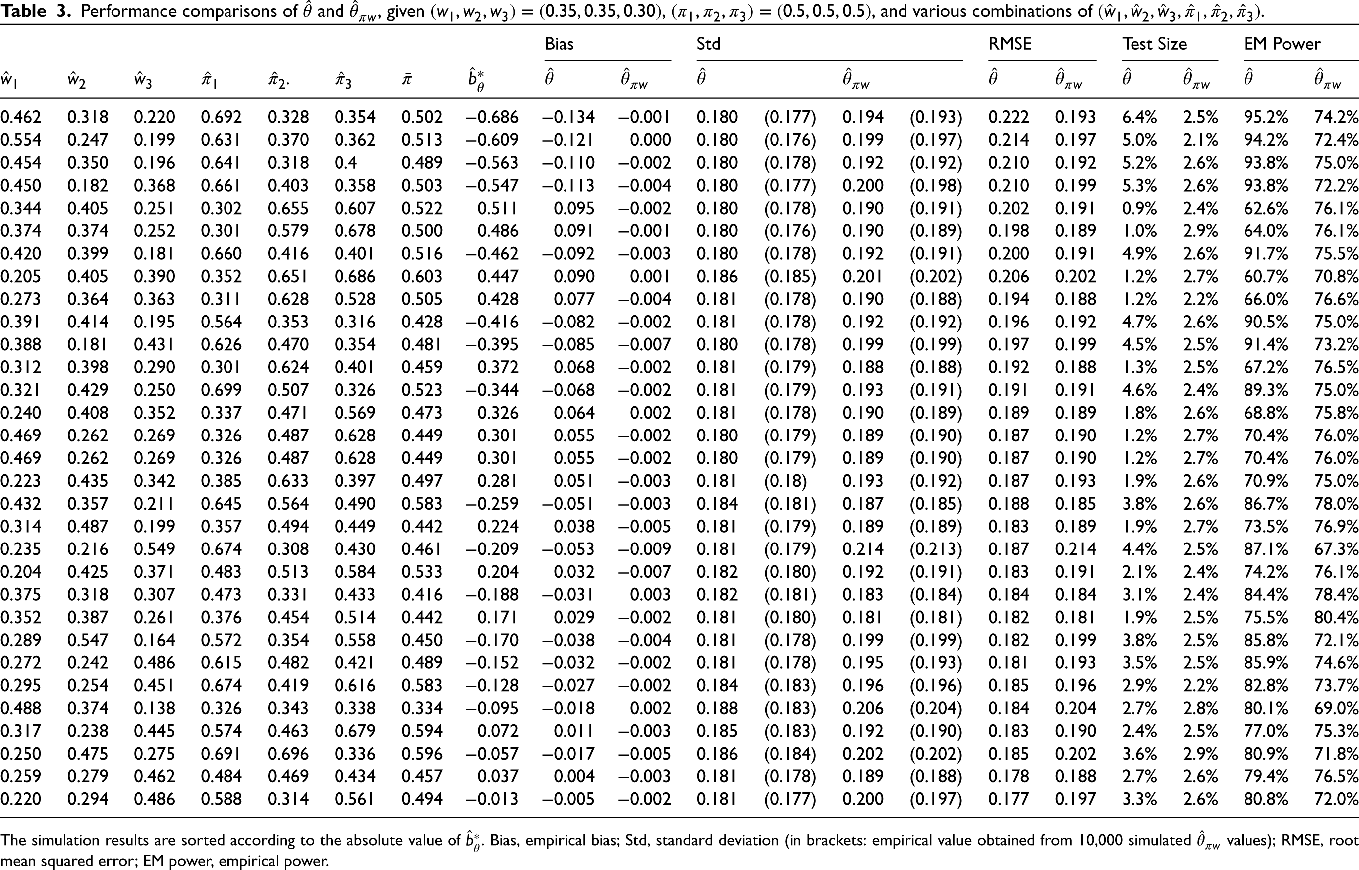
In order to investigate various scenarios that may occur in practice, we generated different combinations of $\{({\hat{w}}_k,{\hat{\pi }}_k),k=1,2,3\}$ . The observed regional weights ${\hat{w}}_k^{{}^{\mathrm{\prime }}}s$ were randomly generated from a uniform distribution within the range of $[0.1,0.7]$ with a constraint on $\sum {\hat{w}}_k=1$ . This wide range allows us to cover a diverse set of possible values for the observed regional weights. The observed treatment allocation ratios ${\hat{\pi }}_k^{{}^{\mathrm{\prime }}}s$ were randomly generated from a uniform distribution with the mean of 0.5 and the range of $[0.3,0.7]$ . By bounding the observed treatment allocation ratio between this range, we avoid values that are too large or too small, as this indicates a very poor randomization scheme, which is rarely the case in practice. For each combination of $\{({\hat{w}}_k,{\hat{\pi }}_k),k=1,2,3\}$ , we performed 10,000 simulations to assess the performance of the two estimators. The simulation results shown in Table 3 include empirical bias, standard deviation, root mean squared error (RMSE), empirical test size, and empirical power. To interpret the size of the biases, we considered the standardization of ${\hat{b}}_{\theta }$ and defined it as

$${\hat{b}}_{\theta }^{*}=\frac{{\hat{b}}_{\theta }}{{\hat{\sigma }}_{\pi w}}.$$

Table 3.

Performance comparisons of $\hat{\theta }$ and ${\hat{\theta }}_{\pi w}$ , given $(w_1,w_2,w_3)=(0.35,0.35,0.30)$ , $({\pi }_1,{\pi }_2,{\pi }_3)=(0.5,0.5,0.5),$ and various combinations of $({\hat{w}}_1,{\hat{w}}_2,{\hat{w}}_3,{\hat{\pi }}_1,{\hat{\pi }}_2,{\hat{\pi }}_3)$ .

								Bias		Std				RMSE		Test Size		EM Power
${\hat{w}}_1$	${\hat{w}}_2$	${\hat{w}}_3$	${\hat{\pi }}_1$	${\hat{\pi }}_2$ .	${\hat{\pi }}_3$	$\overline{\pi }$	${\hat{b}}_{\theta }*$	$\hat{\theta }$	${\hat{\theta }}_{\pi w}$	$\hat{\theta }$		${\hat{\theta }}_{\pi w}$		$\hat{\theta }$	${\hat{\theta }}_{\pi w}$	$\hat{\theta }$	${\hat{\theta }}_{\pi w}$	$\hat{\theta }$	${\hat{\theta }}_{\pi w}$
0.462	0.318	0.220	0.692	0.328	0.354	0.502	−0.686	−0.134	−0.001	0.180	(0.177)	0.194	(0.193)	0.222	0.193	6.4%	2.5%	95.2%	74.2%
0.554	0.247	0.199	0.631	0.370	0.362	0.513	−0.609	−0.121	0.000	0.180	(0.176)	0.199	(0.197)	0.214	0.197	5.0%	2.1%	94.2%	72.4%
0.454	0.350	0.196	0.641	0.318	0.4	0.489	−0.563	−0.110	−0.002	0.180	(0.178)	0.192	(0.192)	0.210	0.192	5.2%	2.6%	93.8%	75.0%
0.450	0.182	0.368	0.661	0.403	0.358	0.503	−0.547	−0.113	−0.004	0.180	(0.177)	0.200	(0.198)	0.210	0.199	5.3%	2.6%	93.8%	72.2%
0.344	0.405	0.251	0.302	0.655	0.607	0.522	0.511	0.095	−0.002	0.180	(0.178)	0.190	(0.191)	0.202	0.191	0.9%	2.4%	62.6%	76.1%
0.374	0.374	0.252	0.301	0.579	0.678	0.500	0.486	0.091	−0.001	0.180	(0.176)	0.190	(0.189)	0.198	0.189	1.0%	2.9%	64.0%	76.1%
0.420	0.399	0.181	0.660	0.416	0.401	0.516	−0.462	−0.092	−0.003	0.180	(0.178)	0.192	(0.191)	0.200	0.191	4.9%	2.6%	91.7%	75.5%
0.205	0.405	0.390	0.352	0.651	0.686	0.603	0.447	0.090	0.001	0.186	(0.185)	0.201	(0.202)	0.206	0.202	1.2%	2.7%	60.7%	70.8%
0.273	0.364	0.363	0.311	0.628	0.528	0.505	0.428	0.077	−0.004	0.181	(0.178)	0.190	(0.188)	0.194	0.188	1.2%	2.2%	66.0%	76.6%
0.391	0.414	0.195	0.564	0.353	0.316	0.428	−0.416	−0.082	−0.002	0.181	(0.178)	0.192	(0.192)	0.196	0.192	4.7%	2.6%	90.5%	75.0%
0.388	0.181	0.431	0.626	0.470	0.354	0.481	−0.395	−0.085	−0.007	0.180	(0.178)	0.199	(0.199)	0.197	0.199	4.5%	2.5%	91.4%	73.2%
0.312	0.398	0.290	0.301	0.624	0.401	0.459	0.372	0.068	−0.002	0.181	(0.179)	0.188	(0.188)	0.192	0.188	1.3%	2.5%	67.2%	76.5%
0.321	0.429	0.250	0.699	0.507	0.326	0.523	−0.344	−0.068	−0.002	0.181	(0.179)	0.193	(0.191)	0.191	0.191	4.6%	2.4%	89.3%	75.0%
0.240	0.408	0.352	0.337	0.471	0.569	0.473	0.326	0.064	0.002	0.181	(0.178)	0.190	(0.189)	0.189	0.189	1.8%	2.6%	68.8%	75.8%
0.469	0.262	0.269	0.326	0.487	0.628	0.449	0.301	0.055	−0.002	0.180	(0.179)	0.189	(0.190)	0.187	0.190	1.2%	2.7%	70.4%	76.0%
0.469	0.262	0.269	0.326	0.487	0.628	0.449	0.301	0.055	−0.002	0.180	(0.179)	0.189	(0.190)	0.187	0.190	1.2%	2.7%	70.4%	76.0%
0.223	0.435	0.342	0.385	0.633	0.397	0.497	0.281	0.051	−0.003	0.181	(0.18)	0.193	(0.192)	0.187	0.193	1.9%	2.6%	70.9%	75.0%
0.432	0.357	0.211	0.645	0.564	0.490	0.583	−0.259	−0.051	−0.003	0.184	(0.181)	0.187	(0.185)	0.188	0.185	3.8%	2.6%	86.7%	78.0%
0.314	0.487	0.199	0.357	0.494	0.449	0.442	0.224	0.038	−0.005	0.181	(0.179)	0.189	(0.189)	0.183	0.189	1.9%	2.7%	73.5%	76.9%
0.235	0.216	0.549	0.674	0.308	0.430	0.461	−0.209	−0.053	−0.009	0.181	(0.179)	0.214	(0.213)	0.187	0.214	4.4%	2.5%	87.1%	67.3%
0.204	0.425	0.371	0.483	0.513	0.584	0.533	0.204	0.032	−0.007	0.182	(0.180)	0.192	(0.191)	0.183	0.191	2.1%	2.4%	74.2%	76.1%
0.375	0.318	0.307	0.473	0.331	0.433	0.416	−0.188	−0.031	0.003	0.182	(0.181)	0.183	(0.184)	0.184	0.184	3.1%	2.4%	84.4%	78.4%
0.352	0.387	0.261	0.376	0.454	0.514	0.442	0.171	0.029	−0.002	0.181	(0.180)	0.181	(0.181)	0.182	0.181	1.9%	2.5%	75.5%	80.4%
0.289	0.547	0.164	0.572	0.354	0.558	0.450	−0.170	−0.038	−0.004	0.181	(0.178)	0.199	(0.199)	0.182	0.199	3.8%	2.5%	85.8%	72.1%
0.272	0.242	0.486	0.615	0.482	0.421	0.489	−0.152	−0.032	−0.002	0.181	(0.178)	0.195	(0.193)	0.181	0.193	3.5%	2.5%	85.9%	74.6%
0.295	0.254	0.451	0.674	0.419	0.616	0.583	−0.128	−0.027	−0.002	0.184	(0.183)	0.196	(0.196)	0.185	0.196	2.9%	2.2%	82.8%	73.7%
0.488	0.374	0.138	0.326	0.343	0.338	0.334	−0.095	−0.018	0.002	0.188	(0.183)	0.206	(0.204)	0.184	0.204	2.7%	2.8%	80.1%	69.0%
0.317	0.238	0.445	0.574	0.463	0.679	0.594	0.072	0.011	−0.003	0.185	(0.183)	0.192	(0.190)	0.183	0.190	2.4%	2.5%	77.0%	75.3%
0.250	0.475	0.275	0.691	0.696	0.336	0.596	−0.057	−0.017	−0.005	0.186	(0.184)	0.202	(0.202)	0.185	0.202	3.6%	2.9%	80.9%	71.8%
0.259	0.279	0.462	0.484	0.469	0.434	0.457	0.037	0.004	−0.003	0.181	(0.178)	0.189	(0.188)	0.178	0.188	2.7%	2.6%	79.4%	76.5%
0.220	0.294	0.486	0.588	0.314	0.561	0.494	−0.013	−0.005	−0.002	0.181	(0.177)	0.200	(0.197)	0.177	0.197	3.3%	2.6%	80.8%	72.0%

The simulation results are sorted according to the absolute value of ${\hat{b}}_{\theta }^{*}$ . Bias, empirical bias; Std, standard deviation (in brackets: empirical value obtained from 10,000 simulated ${\hat{\theta }}_{\pi w}$ values); RMSE, root mean squared error; EM power, empirical power.

The value of ${\hat{b}}_{\theta }^{*}$ is also provided in Table 3. Note that the results presented in Table 3 are sorted by the absolute values of ${\hat{b}}_{\theta }^{*}$ .

We started with scenarios where the value of ${\hat{b}}_{\theta }^{*}$ is negative, taking the first row of Table 3 as an example. It can be observed that $\hat{\theta }$ has a bias of $-0.134$ , while ${\hat{\theta }}_{\pi w}$ is almost unbiased. This indicates that our approach successfully corrected the bias. Considering a significance level of $\alpha =2.5\mathrm{\%}$ , the empirical test size of $\hat{\theta }$ is $6.4\mathrm{\%}$ , and the empirical test size of ${\hat{\theta }}_{\pi w}$ is $2.5\mathrm{\%}$ . The inflated test size of $\hat{\theta }$ is primarily due to its large negative bias. In terms of standard deviation, ${\hat{\theta }}_{\pi w}$ has a slightly higher value of 0.193 compared to 0.177 for $\hat{\theta }$ . The RMSE of ${\hat{\theta }}_{\pi w}$ is 0.193, which is less than the value of 0.222 for $\hat{\theta }$ . The estimator $\hat{\theta }$ has the empirical power of $95.2\mathrm{\%}$ , while ${\hat{\theta }}_{\pi w}$ has the empirical power of $74.2\mathrm{\%}$ . To explain the unusually high empirical power of $\hat{\theta }$ , we need to look at its corresponding test size and standard deviation. When the test size is as high as $6.4\mathrm{\%}$ , such high power is not meaningful.

Next, let's turn our attention to the scenarios where the value of ${\hat{b}}_{\theta }^{*}$ is positive, taking the fifth row of Table 3 as an example. The naïve estimator $\hat{\theta }$ is overestimated with a bias of 0.095, resulting in the empirical test size of $0.9\mathrm{\%}$ , which is well below $2.5\mathrm{\%}$ . The excessively small test size of $\hat{\theta }$ leads to the empirical power of $62.6\mathrm{\%}$ , which is well below the desired power of $80\mathrm{\%}$ . In contrast, ${\hat{\theta }}_{\pi w}$ is nearly unbiased with the empirical test size of $2.4\mathrm{\%}$ and the empirical power of $76.1\mathrm{\%}$ .

Across all the combinations of $\{({\hat{w}}_k,{\hat{\pi }}_k),k=1,2,3\}$ presented in Table 3, regardless of the value of ${\hat{b}}_{\theta }^{*}$ , it is evident that our proposed estimator ${\hat{\theta }}_{\pi w}$ is almost unbiased. When the observed patient assignments $\{({\hat{w}}_k,{\hat{\pi }}_k),k=1,2,3\}$ remarkably deviate from the designed assignments $\{(w_k,{\pi }_k),k=1,2,3\}$ , indicated by ${\hat{b}}_{\theta }^{*}$ being far from 0, the proposed estimator clearly outperforms the naïve estimator. The empirical test size of ${\hat{\theta }}_{\pi w}$ is always close to $2.5\mathrm{\%}$ compared to that of $\hat{\theta }$ . The empirical power of ${\hat{\theta }}_{\pi w}$ is more meaningful when the test size is stable and close to $2.5\mathrm{\%}$ compared to that of $\hat{\theta }$ . However, the standard deviation of ${\hat{\theta }}_{\pi w}$ is slightly greater than that of $\hat{\theta }$ . This is because our approach sacrifices some precision in the process of bias adjustment. Therefore, when there is almost no bias ( ${\hat{b}}_{\theta }^{*}$ is close to 0), the RMSE of ${\hat{\theta }}_{\pi w}$ will be slightly larger than that of $\hat{\theta }$ .

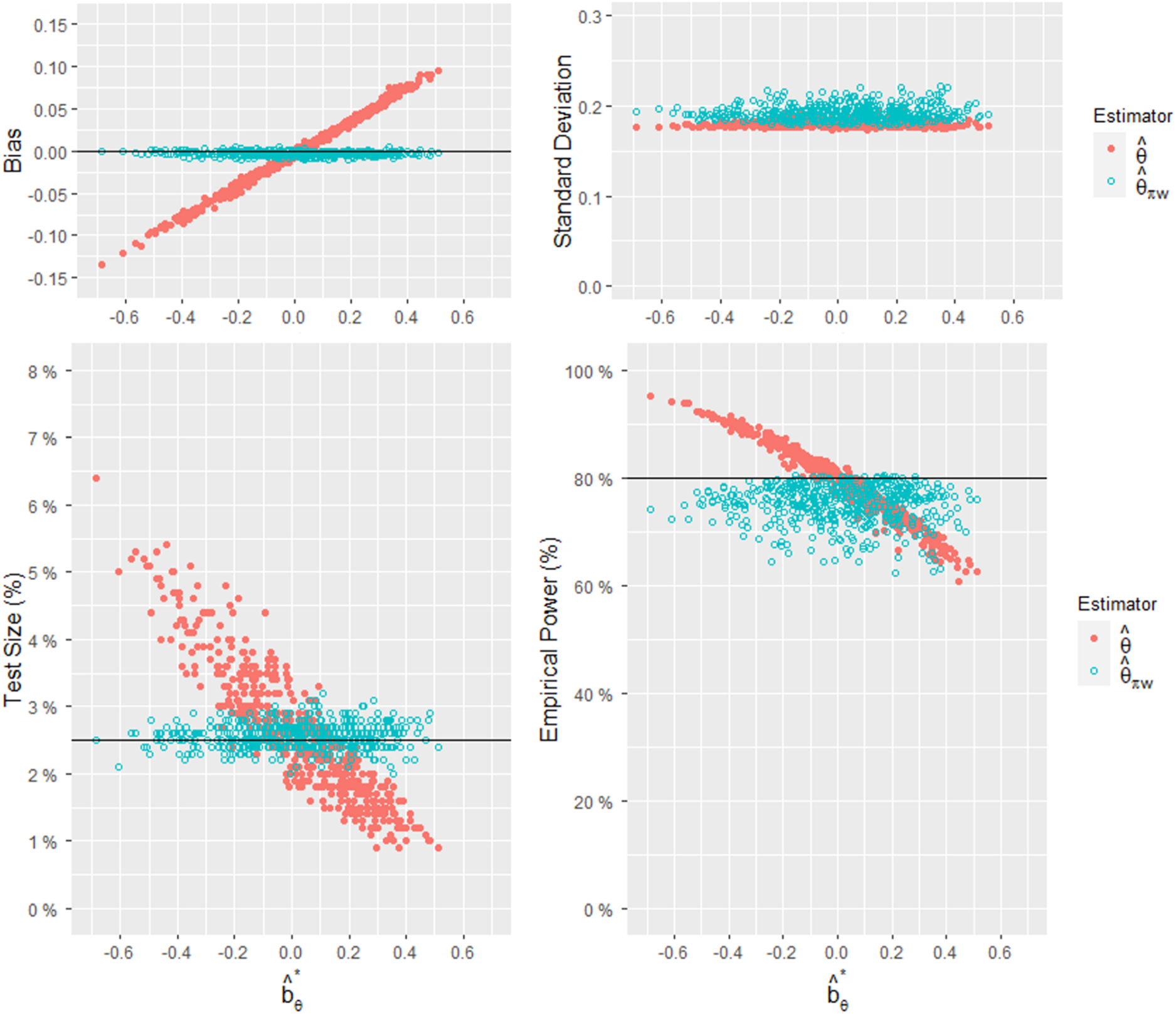
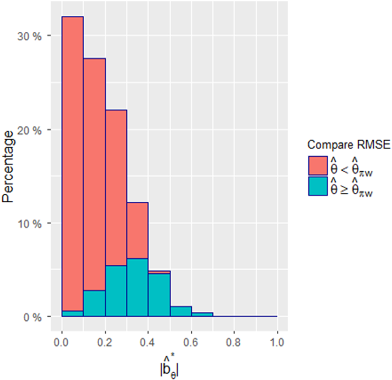
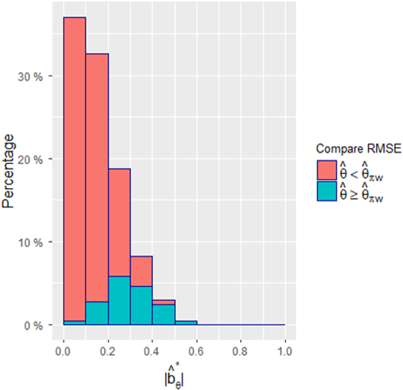
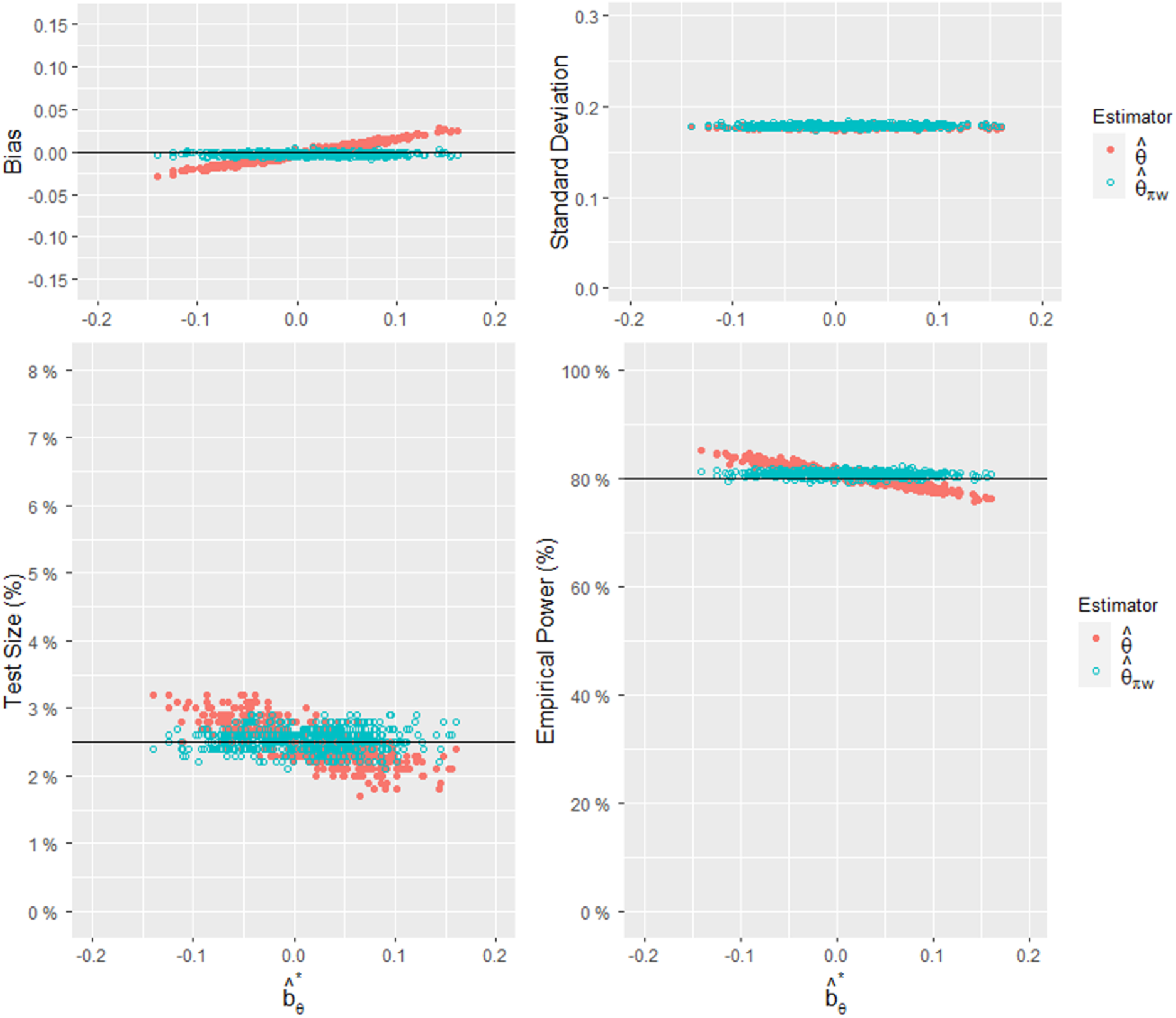
These results can also be clearly seen in Figure 1, where the x-axis represents ${\hat{b}}_{\theta }^{*}$ and each dot represents a combination of $\{({\hat{w}}_k,{\hat{\pi }}_k),k=1,2,3\}$ . A total of 500 combinations were compared between the two estimators, and each combination represents the result of 10,000 simulations. Figure 1 depicts the relationships between ${\hat{b}}_{\theta }^{*}$ and the empirical bias, standard deviation, test size, and power. When the size of bias ${\hat{b}}_{\theta }^{*}$ is far from 0, the empirical test size of $\hat{\theta }$ is far from $2.5\mathrm{\%}$ and the empirical power of $\hat{\theta }$ is far from $80\mathrm{\%}$ . On the other hand, since the empirical test size of the biased-adjusted estimator ${\hat{\theta }}_{\pi w}$ is stable around $2.5\mathrm{\%}$ , the empirical power of ${\hat{\theta }}_{\pi w}$ is statistically informative. Figure 2 displays a histogram comparing the RMSEs of the two estimators for the 500 combinations. Since the RMSE is affected by the bias and standard deviation and our approach sacrifices some precision in the process of adjusting the bias, our approach will show a greater advantage when $|{\hat{b}}_{\theta }^{*}|$ is large.

Figure 1.

Comparisons of the empirical bias, standard deviation, test size, and power of $\hat{\theta }$ and ${\hat{\theta }}_{\pi w}$ , given $(w_1,w_2,w_3)=(0.35,0.35,0.30)$ , $({\pi }_1,{\pi }_2,{\pi }_3)=(0.5,0.5,0.5),$ and 500 combinations of $({\hat{w}}_1,{\hat{w}}_2,{\hat{w}}_3,{\hat{\pi }}_1,{\hat{\pi }}_2,{\hat{\pi }}_3)$ .

Figure 2.

Comparisons of the RMSEs of $\hat{\theta }$ and ${\hat{\theta }}_{\pi w}$ when $(w_1,w_2,w_3)=(0.35,0.35,0.30)$ and $({\pi }_1,{\pi }_2,{\pi }_3)=(0.5,0.5,0.5)$ . The absolute values of ${\hat{b}}_{\theta }^{*}$ were obtained from 500 combinations of $({\hat{w}}_1,{\hat{w}}_2,{\hat{w}}_3,{\hat{\pi }}_1,{\hat{\pi }}_2,{\hat{\pi }}_3)$ . The darker area means that the RMSE value of $\hat{\theta }$ is greater than or equal to ${\hat{\theta }}_{\pi w}$ ; otherwise, it is represented by the lighter area.

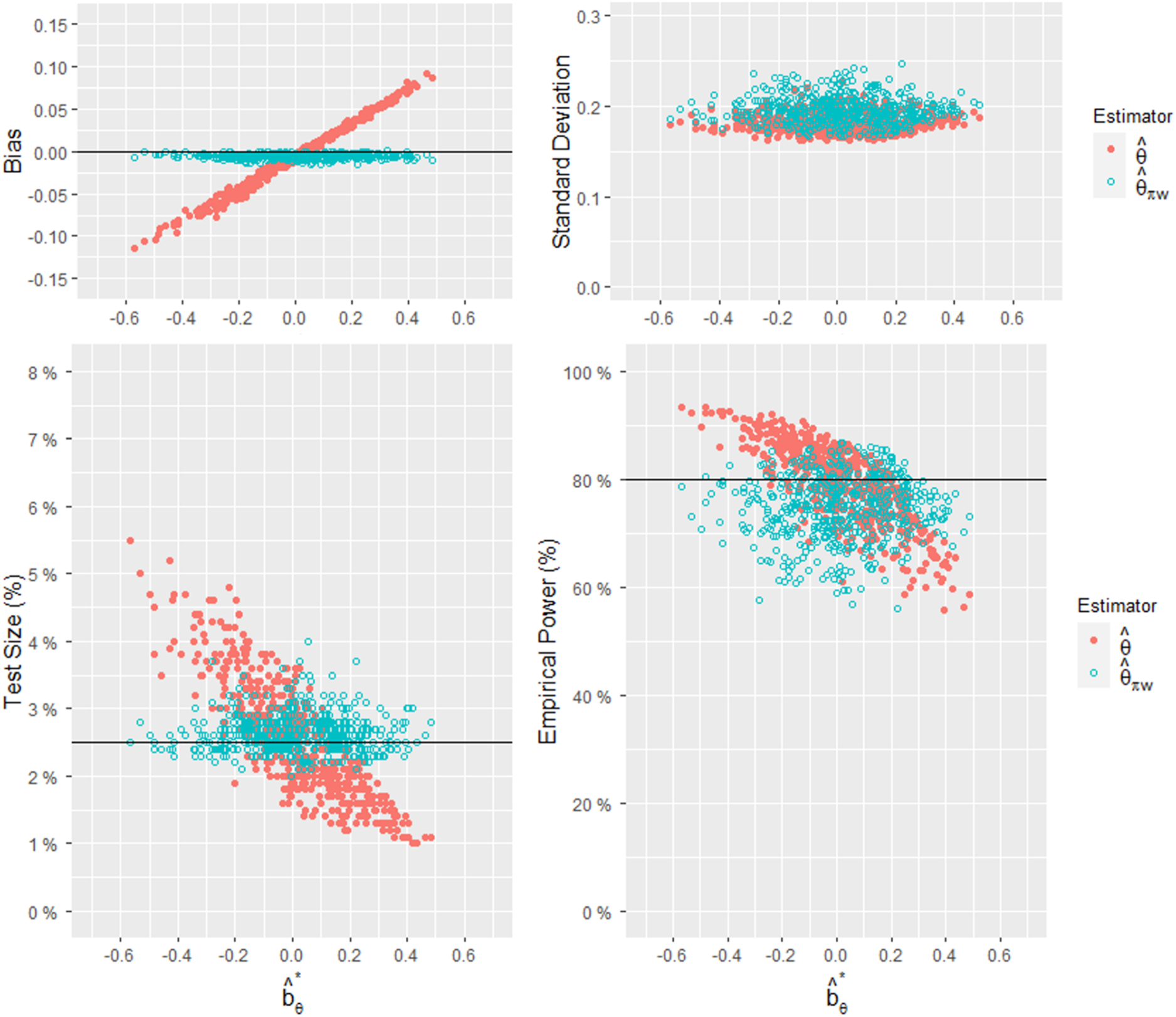
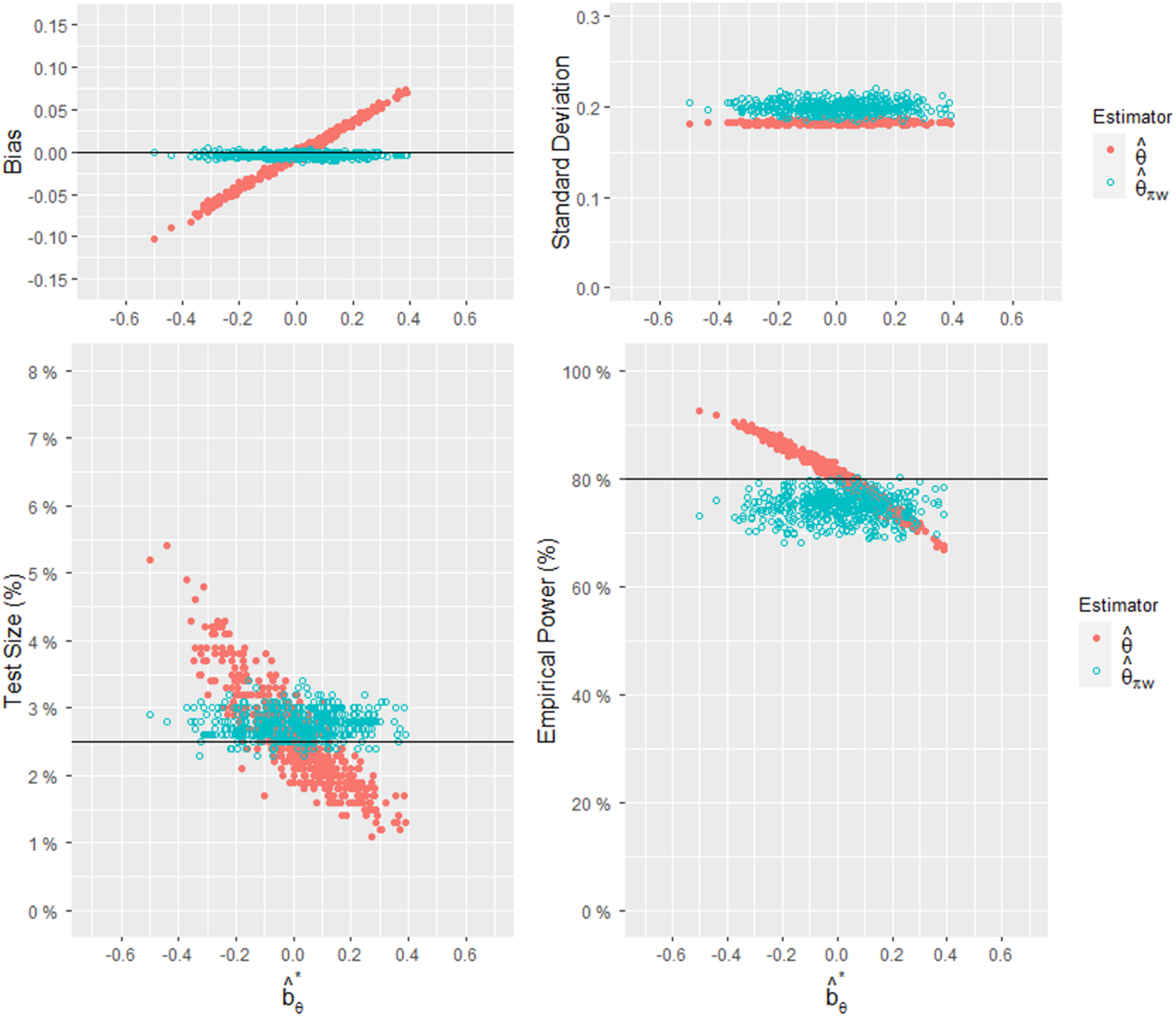
In the second set of predetermined patient allocation settings, we have $(w_1,w_2,w_3)=(0.35,0.35,0.30)$ and $({\pi }_1,{\pi }_2,{\pi }_3)=(0.7,0.7,0.7)$ . We conducted 10,000 simulations for each combination $\{({\hat{w}}_k,{\hat{\pi }}_k),k=1,2,3\}$ , considering a total of 500 combinations for analysis. For this set, the observed regional weights ${\hat{w}}_k^{{}^{\mathrm{\prime }}}s$ were randomly generated from a uniform distribution within the range of $[0.1,0.7]$ with a constraint on $\sum {\hat{w}}_k=1$ . The observed treatment allocation ratios ${\hat{\pi }}_k^{{}^{\mathrm{\prime }}}s$ were randomly generated from a uniform distribution with the mean of 0.7, and the range of $[0.55,0.85]$ . The required sample size $N_{ne}$ was determined to be 667. The results of the simulation study are presented in Figures 3 and 4. Figure 3 illustrates the relationships between ${\hat{b}}_{\theta }^{*}$ and the bias, standard deviation, test size, and power for the two estimators ${\hat{\theta }}_{\pi w}$ and $\hat{\theta }$ . Figure 4 presents a histogram comparing the RMSEs of the two estimators for the 500 combinations of $\{({\hat{w}}_k,{\hat{\pi }}_k),k=1,2,3\}$ . Similar to the previous analysis, the findings shown in Figures 3 and 4 align with the conclusions drawn from Figures 1 and 2.

Figure 3.

Comparisons of the empirical bias, standard deviation, test size, and power of $\hat{\theta }$ and ${\hat{\theta }}_{\pi w}$ , given $(w_1,w_2,w_3)=(0.35,0.35,0.30)$ , $({\pi }_1,{\pi }_2,{\pi }_3)=(0.7,0.7,0.7),$ and 500 combinations of $({\hat{w}}_1,{\hat{w}}_2,{\hat{w}}_3,{\hat{\pi }}_1,{\hat{\pi }}_2,{\hat{\pi }}_3)$ .

Figure 4.

Comparisons of the RMSEs of $\hat{\theta }$ and ${\hat{\theta }}_{\pi w}$ when $(w_1,w_2,w_3)=(0.35,0.35,0.30)$ and $({\pi }_1,{\pi }_2,{\pi }_3)=(0.7,0.7,0.7)$ . The absolute values of ${\hat{b}}_{\theta }^{*}$ were obtained from 500 combinations of $({\hat{w}}_1,{\hat{w}}_2,{\hat{w}}_3,{\hat{\pi }}_1,{\hat{\pi }}_2,{\hat{\pi }}_3)$ . The darker area means that the RMSE value of $\hat{\theta }$ is greater than or equal to ${\hat{\theta }}_{\pi w}$ ; otherwise, it is represented by the lighter area.

When the observed regional weights ${\hat{w}}_k^{{}^{\mathrm{\prime }}}s$ and treatment allocation ratios ${\hat{\pi }}_k^{{}^{\mathrm{\prime }}}s$ closely align with the design, the bias of ${\hat{b}}_{\theta }^{*}$ is close to 0, and our proposed estimator ${\hat{\theta }}_{\pi w}$ demonstrates its advantages by reducing bias, maintaining a stable test size close to $2.5\mathrm{\%}$ , and providing informative empirical power. To demonstrate this, we adopted the same designed set as the first set in this section, and assumed the observed regional weights ${\hat{w}}_k^{{}^{\mathrm{\prime }}}s$ were randomly generated from a uniform distribution within the range of $[0.25,0.40]$ , the observed treatment allocation ratios ${\hat{\pi }}_k^{{}^{\mathrm{\prime }}}s$ were randomly generated from a uniform distribution within the range of $[0.45,0.55]$ . Such assumptions about the range of observed values ${\hat{w}}_k^{{}^{\mathrm{\prime }}}s$ and ${\hat{\pi }}_k^{{}^{\mathrm{\prime }}}s$ are not exceptional but rather represent a common scenario. The results are summarized in Figure 5, which illustrates the relationships between ${\hat{b}}_{\theta }^{*}$ and the bias, standard deviation, test size, and power for the two estimators ${\hat{\theta }}_{\pi w}$ and $\hat{\theta }$ . The stability is demonstrated by the consistent performance of our method despite the variability of ${\hat{b}}_{\theta }^{*}$ . Therefore, our method demonstrates better performance.

Figure 5.

Comparisons of the empirical bias, standard deviation, test size, and power of $\hat{\theta }$ and ${\hat{\theta }}_{\pi w}$ , given $(w_1,w_2,w_3)=(0.35,0.35,0.30)$ , $({\pi }_1,{\pi }_2,{\pi }_3)=(0.5,0.5,0.5),$ and 500 combinations of $({\hat{w}}_k,{\hat{\pi }}_k),k=1,2,3$ , where $0.25\le {\hat{w}}_k\le 0.40$ and $0.45\le {\hat{\pi }}_k\le 0.55$ .

In the third set of predetermined patient allocation settings, we considered seven regions to investigate the scenario with a larger number of regions. Let the event rates of the treatment group and the control group be $\{p_{Tk}\}=(0.50,0.50,0.50,0.60,0.60,0.60,0.60)$ and $\{p_{Ck}\}=(0.65,0.65,0.65,0.70,0.70,0.70,0.70),$ respectively. At the design stage, we set the patient assignments as $w_i=1/7$ and ${\pi }_i=0.5,i=1,\dots ,7$ . The between-region variance ${\tau }^2$ was 0.0077. At a significance level of $\alpha =2.5\mathrm{\%}$ and a power of $1-\beta =80\mathrm{\%}$ , the required sample size $N_{ne}$ was determined to be 523. The observed regional weights ${\hat{w}}_k^{{}^{\mathrm{\prime }}}s$ were randomly generated from a uniform distribution within the range of $[0.1,0.7]$ with a constraint on $\sum {\hat{w}}_k=1$ . The observed treatment allocation ratios ${\hat{\pi }}_k^{{}^{\mathrm{\prime }}}s$ were randomly generated from a uniform distribution with the mean of 0.5, and the range of $[0.3,0.7]$ . The results of the simulation study are presented in Figure 6, which illustrates the relationships between ${\hat{b}}_{\theta }^{*}$ and the bias, standard deviation, test size, and power for the two estimators ${\hat{\theta }}_{\pi w}$ and $\hat{\theta }$ . Since our approach sacrifices some precision in the process of bias adjustment, this effect appears to be more pronounced as the number of regions increases. However, the performance of our proposed estimator remains stable, across different values of ${\hat{b}}_{\theta }^{*}$ .

Figure 6.

Comparisons of the empirical bias, standard deviation, test size, and power of $\hat{\theta }$ and ${\hat{\theta }}_{\pi w}$ , given $w_i=1/7$ and ${\pi }_i=0.5,i=1,\dots ,7,$ and 500 combinations of $({\hat{w}}_k,{\hat{\pi }}_k),k=1,2,\dots ,7$ .

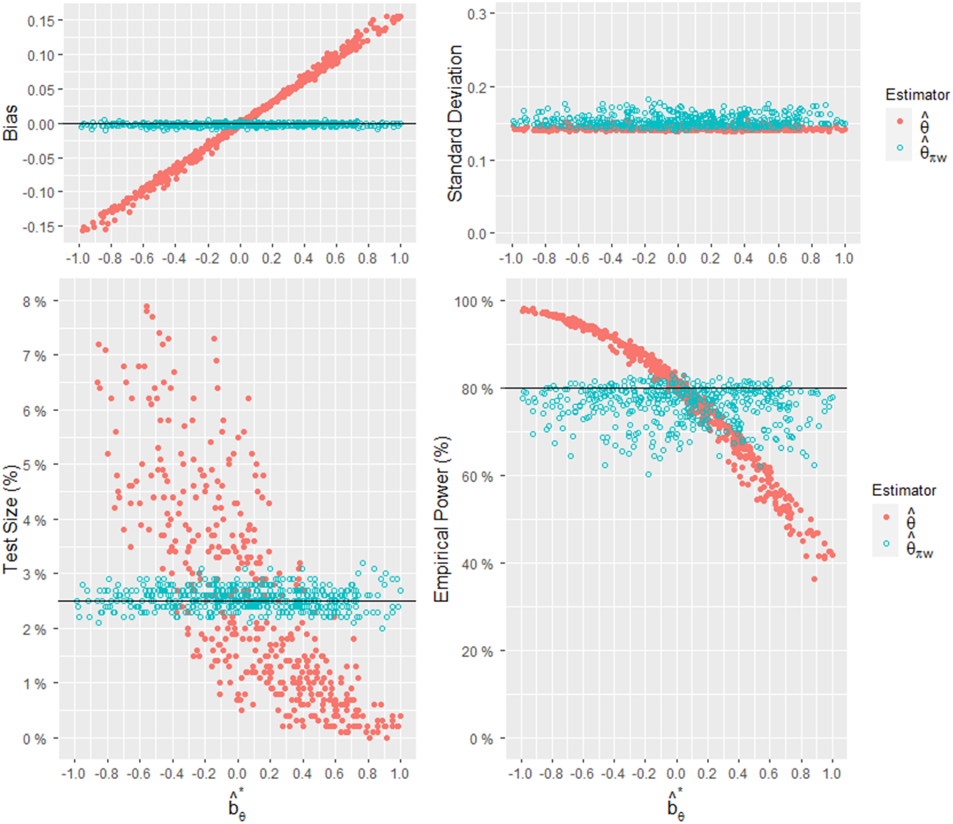
Finally, we considered the scenario with noticeable treatment effect heterogeneity in the case of three regions with $\{p_{Tk}\}=(0.45,0.60,0.65)$ and $\{p_{Ck}\}=(0.60,0.65,0.75)$ . At the design stage, we set the patient assignments as $(w_1,w_2,w_3)=(0.35,0.35,0.30)$ and $({\pi }_1,{\pi }_2,{\pi }_3)=(0.5,0.5,0.5)$ . The between-region variance ${\tau }^2$ was 0.0280. Notably, this value is nearly four times greater than ${\tau }^2=0.0071$ in the first designed set. At a significance level of $\alpha =2.5\mathrm{\%}$ and a power of $1-\beta =80\mathrm{\%}$ , the required sample size $N_{ne}$ was determined to be 839. The observed regional weights ${\hat{w}}_k^{{}^{\mathrm{\prime }}}s$ were randomly generated from a uniform distribution within the range of $[0.1,0.7]$ . The observed treatment allocation ratios ${\hat{\pi }}_k^{{}^{\mathrm{\prime }}}s$ were randomly generated from a uniform distribution with the mean of 0.5 and the range of $[0.3,0.7]$ . The results of the simulation study are presented in Figure 7, which illustrates the relationships between ${\hat{b}}_{\theta }^{*}$ and the bias, standard deviation, test size, and power for the two estimators ${\hat{\theta }}_{\pi w}$ and $\hat{\theta }$ . In this scenario with obvious treatment effect heterogeneity, our method continues to demonstrate advantages in reducing bias, ensuring that the test size is stable at around 2.5%, and providing meaningful empirical power.

Figure 7.

Comparisons of the empirical bias, standard deviation, test size, and power of $\hat{\theta }$ and ${\hat{\theta }}_{\pi w}$ , given $p_{Tk}=(0.45,0.60,0.65)$ , $p_{Ck}=(0.60,0.65,0.75),$ and 500 combinations of $({\hat{w}}_k,{\hat{\pi }}_k),k=1,2,3$ .

In summary, the simulation study provides evidence that the bias-adjusted estimator ${\hat{\theta }}_{\pi w}$ outperforms the naïve estimator $\hat{\theta }$ by reducing the bias, maintaining a stable test size close to 2.5%, and yielding informative empirical power. The larger the bias is, the more advantageous the proposed method is.

5. Example

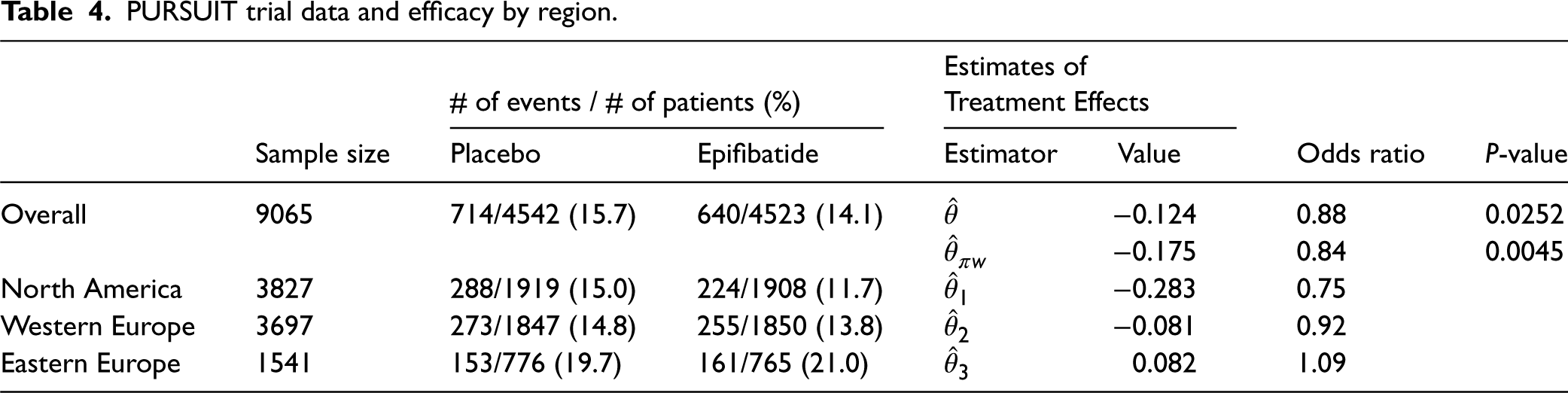
In this section, we provide a real-data example to illustrate the proposed approach. We utilized partial information from the Platelet Glycoprotein IIb/IIIa in Unstable Angina: Receptor Suppression Using Integrilin Therapy (PURSUIT) trial.^16,17,18 The PURSUIT trial was a randomized, double-blind, add-on, MRCT that enrolled a total of 10,948 patients with acute coronary syndrome from 726 hospitals across 28 countries. The data is available online at https://doi.org/10.1056/NEJM199808133390704. In this example, we focused on 9065 patients who participated in the trial from three geographical regions: North America (NA), Western Europe (WE), and Eastern Europe (EE). In addition to standard therapy, the patients received eptifibatide or placebo in a 1:1 treatment allocation ratio. The primary endpoint was a composite of death and nonfatal myocardial infarction (MI) at 30 days after study initiation. Table 4 shows the event rates (death or MI) and the number of patients for the overall trial population as well as the individual regions (NA, WE, and EE). Based on this information, the observed regional weights were $({\hat{w}}_1,{\hat{w}}_2,{\hat{w}}_3)=(0.422,0.408,0.170)$ and the observed treatment allocation ratios were $({\hat{\pi }}_1,{\hat{\pi }}_2,{\hat{\pi }}_3)=(0.499,0.500,0.496)$ . The treatment allocation ratio for each region was approximately 0.5, indicating that the randomization scheme worked well. Additionally, the overall treatment allocation ratio was $\overline{\pi }=0.499$ .

Table 4.

PURSUIT trial data and efficacy by region.

		# of events / # of patients (%)		Estimates of Treatment Effects
	Sample size	Placebo	Epifibatide	Estimator	Value	Odds ratio	P-value
Overall	$9065$	714/4542 (15.7)	640/4523 (14.1)	$\hat{\theta }$	−0.124	0.88	0.0252
				${\hat{\theta }}_{\pi w}$	−0.175	0.84	0.0045
North America	3827	288/1919 (15.0)	224/1908 (11.7)	${\hat{\theta }}_1$	−0.283	0.75
Western Europe	3697	273/1847 (14.8)	255/1850 (13.8)	${\hat{\theta }}_2$	−0.081	0.92
Eastern Europe	1541	153/776 (19.7)	161/765 (21.0)	${\hat{\theta }}_3$	0.082	1.09

Table 4 also provides the estimates of the treatment effects both overall and by region. Note that the treatment effect is defined as the log(OR) of the eptifibatide group compared to that of the placebo group, with a lower value indicating a better result. Based on the DREM with the regional treatment effect estimates $({\hat{\theta }}_1,{\hat{\theta }}_2,{\hat{\theta }}_3)$ , the between-region variance estimate ${\hat{\tau }}^2$ was 0.0187. In addition, the naïve estimate $\hat{\theta }$ for log(OR) was $-0.124$ , with the standard error of 0.063 and the P-value of 0.0252. The corresponding estimate of OR was 0.88. For our purpose, we assumed that predetermined regional weights in the protocol were $(w_1,w_2,w_3)=(0.6,0.3,0.1).$ Using these regional weights, the bias-adjusted estimate ${\hat{\theta }}_{\pi w}$ was calculated to be $-0.175$ , with the standard error of 0.067 and the P-value of 0.0045. The corresponding estimate $exp({\hat{\theta }}_{\pi w})$ was 0.84. Notably, the P-value for ${\hat{\theta }}_{\pi w}$ is much less than that for $\hat{\theta }$ , indicating a more significant overall treatment effect when the bias-adjusted estimate was used. In principle, if we use $\alpha =2.5\mathrm{\%}$ for testing the significance of the treatment effect, $\hat{\theta }$ did not lead to the conclusion of significance. However, the proposed method concluded a high significance.

6. Discussion

With the framework of the DREM, we expanded the approach proposed by Tian et al. ⁶ to evaluate an MRCT. Specifically, we proposed the adjusted estimator ${\hat{\theta }}_{\pi w}$ that quantifies the bias of the naïve estimator $\hat{\theta }$ through conditional inference. The bias-adjusted estimator improves the accuracy of the treatment effect estimation, as it is stochastically closer to the true treatment effect $\theta$ . This conditional correction of bias further strengthens our understanding of the process of enhancing the accuracy.

In this work, we also derived the required sample sizes $N_{\pi w}$ and $N_{ne}$ for ${\hat{\theta }}_{\pi w}$ and $\hat{\theta }$ , respectively, to achieve the desired power level. Through simulation analysis considering different combinations of observed patient assignments, we evaluated the performance of the two estimators. The bias-adjusted estimator exhibited a reduced bias, maintained a stable test size close to the target significance level, and provided meaningful empirical power. These findings emphasize the importance of bias correction in MRCTs and highlight the effectiveness of our proposed approach for obtaining accurate treatment effect estimates. Our approach is especially valuable when there is noticeable bias in patient assignments. Furthermore, our approach is flexible and can be applied to MRCTs with different numbers of regions ( $K>3$ ) and other types of endpoints, such as continuous or survival outcomes.

There are numerous challenges in the design and evaluation of MRCTs. The “Basic Principles of Global Clinical Trials” issued by the Japanese Ministry of Health, Labour and Welfare (MHLW), ¹⁹ provides some guidelines for the planning and implementation of global clinical studies. These guidelines raise concerns regarding the consistency of efficacy for patients in a specific region and the overall population. In future research, incorporating the bias-adjusted estimator proposed in this paper may contribute to exploration of this topic and aid in the design of MRCTs. Of note, some informative studies by Tsong et al., ²⁰ Tsou et al., ²¹ and Liu et al. ⁴ have investigated the consistency of efficacy across regions, providing valuable insights.