Weighting methods for truncation by death in cluster-randomized trials

Abstract

Patient-centered outcomes, such as quality of life and length of hospital stay, are the focus in a wide array of clinical studies. However, participants in randomized trials for elderly or critically and severely ill patient populations may have truncated or undefined non-mortality outcomes if they do not survive through the measurement time point. To address truncation by death, the survivor average causal effect has been proposed as a causally interpretable subgroup treatment effect defined under the principal stratification framework. However, the majority of methods for estimating the survivor average causal effect have been developed in the context of individually randomized trials. Only limited discussions have been centered around cluster-randomized trials, where methods typically involve strong distributional assumptions for outcome modeling. In this article, we propose two weighting methods to estimate the survivor average causal effect in cluster-randomized trials that obviate the need for potentially complicated outcome distribution modeling. We establish the requisite assumptions that address latent clustering effects to enable point identification of the survivor average causal effect, and we provide computationally efficient asymptotic variance estimators for each weighting estimator. In simulations, we evaluate our weighting estimators, demonstrating their finite-sample operating characteristics and robustness to certain departures from the identification assumptions. We illustrate our methods using data from a cluster-randomized trial to assess the impact of a sedation protocol on mechanical ventilation among children with acute respiratory failure.

1. Introduction

In cluster-randomized trials (CRTs), groups of individuals, such as schools, communities, or health facilities, are randomly assigned to treatments. ¹ CRTs are a favorable alternative to individually randomized trials when the intervention must be administered to entire groups, there are concerns about contamination (i.e. individuals can gain access to treatment(s) to which they were not assigned), and/or individual random assignment is logistically challenging. ² In CRTs, researchers may be interested in studying the causal effect of a binary treatment on a non-mortal outcome like quality of life. However, in some applications, individual participants may die before the time when their non-mortal outcome would be measured, and death acts as an intercurrent event. Mortality rates can be substantial in CRTs among vulnerable populations such as the critically ill or elderly patients.

Death prior to follow-up is a post-randomization event that precludes the complete measurement of a non-mortal outcome. However, estimation of treatment effects among observed survivors can introduce selection bias when survival status is impacted by treatment because such conditioning disrupts the balance of confounders, measured and unmeasured, afforded by randomization. Bias due to conditioning on post-randomization variables such as death is a well-documented issue in the causal inference literature.^3,4 To address this problem from a causal perspective, Frangakis and Rubin ⁵ proposed the principal stratification framework which partitions populations with respect to cross-classified potential outcomes of a binary post-randomization variable. These latent strata are thus unaffected by treatment assignment and can be considered as pre-treatment covariates that define relevant subpopulations. In the context of truncation by death, a common causal estimand of interest is the mean difference in potential outcomes among individuals who would survive under either treatment received (referred to as the always-survivors), named the survivor average causal effect (SACE).^6,7 This is precisely the subpopulation where the pair of non-mortality potential outcomes are well-defined without truncation by death.

For the setting of individually randomized trials, several methods have been proposed to point identify and estimate SACE. For example, Zhang et al. ⁸ introduced a mixture model approach for empirical identification of SACE, which relies on correctly specifying the joint distribution of principal strata and non-mortal outcomes conditional on covariates. While likelihood inference leads to efficient estimators under correct model assumptions, accurate specification of the conditional outcome models is usually more challenging than the principal strata model. In addition, empirical identification under the mixture model requires sufficient distance between the mixture components and may be numerically less stable otherwise. ⁹ Alternatively, leveraging information from baseline covariates, Hayden et al. ¹⁰ and Ding and Lu ¹¹ considered different formulations of ignorability assumptions that allow for non-parametric point identification of SACE. These assumptions result in simple weighting methods for these estimands. Employing a similar set of assumptions to Ding and Lu, ¹¹ Zehavi and Nevo ¹² analogously developed matching estimators for SACE. Despite the simplicity of the weighting methods, they were designed for independent and identically distributed (iid) data and may not be directly applicable to the multilevel data structure present in CRTs. In CRTs, individuals within the same group tend to have positively correlated outcomes, even after conditioning on measured individual-level covariates. Failing to properly account for this correlation may result in underestimated variances and anti-conservative inference. ¹³ Moreover, if there are unobserved cluster-level characteristics that simultaneously affect survival statuses and non-mortal outcomes of individuals, the existing SACE estimators based only on individual covariate information for non-parametric identification (as with iid data) would not suffice even under cluster randomization. The role of clustering effects on causal identification of the SACE, particularly from potentially unmeasured sources, has not been sufficiently explored for CRTs.

In this article, we survey the application of weighting estimators for addressing truncation by death in CRTs. We pursue the principal stratification framework and tackle the additional complications associated with the hierarchical data structure imposed by cluster randomization. While there are a number of likelihood-based methods that exist for CRTs with truncation by death,^14–16 the more intuitive weighting estimators for SACE have not been fully studied. To dispense with the need to model the outcome distributions, we provide two weighting estimators derived under different sets of identification assumptions inspired by Hayden et al., ¹⁰ Ding and Lu, ¹¹ and Zehavi and Nevo. ¹² While the estimators are distinct, they turn out to be functions of the exact same working models to predict survival status, and we provide a conceptual and numerical comparison between these estimators. Furthermore, for each estimator, we consider both conditional and marginal logistic regression paradigms for modeling survival status as they are commonly used in analyses of CRTs. ¹ To accomplish this, we solve for the SACE estimators and construct their sandwich variance expressions using cluster-indexed estimating equations per the M-estimation method^17–19 that are specific to each modeling paradigm.

We have organized the remaining sections as follows. In Section 2, we define notation, provide two sets of identification assumptions, and present the corresponding weighting estimators for SACE in CRTs, along with their variance estimators. In Section 3, we conduct a simulation study to empirically assess the performance of our estimators under different data generating mechanisms which adhere to each set of assumptions. Moreover, we assess the necessity of explicitly modeling for latent group-level effects by comparing the inferential performance of the conditional to the marginal model for survival status in the SACE estimators. Although the proposed marginal model does not incorporate these effects directly, the cluster-indexed M-estimation results in a sandwich variance estimator that aims to correct for this in inference. We also directly compare the computing time and coverage of our proposed asymptotic confidence intervals against bootstrap confidence intervals. In Section 4, we apply our methods to SACE estimation in a CRT that evaluates the impact of a sedation protocol on mechanical ventilation duration among children with acute respiratory failure. In the data application, we consider the analysis of a duration outcome defined within a specific time frame and ascribe to it no parametric assumptions. However, we leave a full time-to-event analysis, which includes addressing censoring in causal assumptions as well as estimation, for future development of the survival framework for SACE in CRTs. Section 5 concludes with a discussion. To facilitate implementation of the proposed methods, we provide a companion R package, PtSaceCrts, for implementing our weighting estimators in CRTs, available at https://github.com/abcdane1/PtSaceCrts.

2. Methods

2.1. Notation, survivor average causal effect estimand, and assumptions

We use the following notation for CRTs. Let $n_c$ denote the number of clusters in a study. The subscript $i$ refers to the $i\text{-th}$ cluster such that $i=1,\dots ,n_c$ . Let $n_i<\mathrm{\infty }$ be the size of cluster $i$ , and $A_i\in \{0,1\}$ be the binary treatment assigned to cluster $i$ . The double subscript “ $ij$ ” refers to the $j\text{-th}$ individual, $j=1,\dots ,n_i$ , in the $i\text{-th}$ cluster. In the observed data, let $S_{ij}\in \{0,1\}$ be individual survival status before the measurement of the non-mortal outcome, and let $Y_{ij}$ be the non-mortal outcome. Under the potential outcomes framework, we let $S_{ij}(a)$ and $Y_{ij}(a)$ be the potential values of the survival status and non-mortal outcome, respectively, of individual $j$ in cluster $i$ had cluster $i$ been assigned to $A_i=a$ . Under truncation by death, potential outcomes are connected to observed outcomes under received treatment assignment through the cluster-level SUTVA (the stable unit treatment value assumption), where $S_{ij}=A_i{S}_{ij}(1)+(1-A_i)S_{ij}(0)$ and if $S_{ij}(a)=1$ , then $Y_{ij}=A_i{Y}_{ij}(1)+(1-A_i)Y_{ij}(0)$ . If $S_{ij}(a)=0$ , then we denote $Y_{ij}(a)=*$ since it is not completely measured following established notation for SACE in the independent data setting.^7,8 In addition, we define $S_i(a)=(S_{i1}(a),\dots ,S_{i{n}_i}(a){)}^T$ , and $Y_i(a)=(Y_{i1}(a),\dots ,Y_{i{n}_i}(a){)}^T$ .

Under the principal stratification framework, ⁵ we denote the prinicipal strata in terms of the joint variables, $G_{ij}=(S_{ij}(1),S_{ij}(0))\in \{0,1\}\times \{0,1\}$ . These strata partition the population into subgroups defined with potential post-randomization events (sometimes referred to as intercurrent events) and since they are no longer functions of $A_i=a$ , stratum membership can be viewed as a pre-treatment covariate. The strata are always-survivors when $G_{ij}=(1,1)$ , protected patients when $G_{ij}=(1,0)$ , harmed patients when $G_{ij}=(0,1)$ , and never-survivors when $G_{ij}=(0,0)$ . For studying the treatment effect on the non-mortality outcome, we define the estimand within the sub-population of always-survivors. We restrict the estimand to this stratum because it is the only subgroup for which $Y_{ij}(1)$ and $Y_{ij}(0)$ are both unambiguously defined (or equivalently without impact of the intercurrent event of death). These effects are represented as functions $g(\mu (1),\mu (0))$ where for $a=0,1$ ,

$$\mu (a)=E\{Y_{ij}(a)|G_{ij}=(1,1)\}=\frac{E\{Y_{ij}(a)S_{ij}(1)S_{ij}(0)\}}{E\{S_{ij}(1)S_{ij}(0)\}}$$

(1)

Possible functions $g(\mu (1),\mu (0))$ may be the mean difference or risk ratio. We primarily focus on the SACE expressed in mean difference (although the methods apply directly to other summary measures) defined as

$$\tau =\mu (1)-\mu (0)=E\{Y_{ij}(1)-Y_{ij}(0)|G_{ij}=(1,1)\}$$

(2)

This estimand represents the expected difference in response had an individual received the active treatment as compared to the control given their membership in the sub-population of always-survivors—that is, a subset of healthier patients for whom the definition of non-mortality potential outcomes is not affected by the intercurrent event of death.

Because stratum membership is only partially observed, the estimand $\tau$ cannot be directly identified without additional assumptions. We consider assumptions that require leveraging information from observed baseline covariates. Let the variables $X_{ij}$ denote vectors of individual-level covariates such that $X_i$ is the covariate matrix for all individuals in cluster $i$ , and let the variables $C_i$ denote vectors of cluster-level covariates. In addition to the cluster-level SUTVA, we require that for all $i,j$ and $a=0,1$ that $0<P(S_{ij}(a)=1|X_i,C_i)<1$ . In other words, every individual within every cluster has some possibility of either survival or mortality under both treatments. The remaining assumptions are as follows:

Assumption 1 (Between-cluster independence)

The potential outcomes and cluster-level baseline variables $\{S_i(1),S_i(0),Y_i(1),Y_i(0),X_i,C_i\}$ are independent across clusters and drawn from a common distribution for a given cluster size.

Assumption 2 (Randomization)

Treatment assignment is independent of all cluster-level variables such that $A_i\perp \{S_i(1),S_i(0),Y_i(1),Y_i(0),X_i,C_i\}$ , and $P(A_i=1)=p\in (0,1)$ .

Assumption 3 (Non-informative cluster-size)

Within each cluster $i$ , the vector of the individual-level potential outcomes $\{S_{ij}(1),S_{ij}(0),Y_{ij}(1),Y_{ij}(0)\}$ have the same marginal distribution that is independent of the cluster size $n_i$ .

Assumptions 1 and 2 are standard assumptions for CRTs. Assumption 3 prevents the size of each cluster from possibly affecting individuals’ survival status and non-mortal outcomes, a phenomenon referred to as informative cluster size. ²⁰ This assumption thus allows us to define $\mu (a)$ as a ratio of marginal expectations of individual-level potential outcomes without ambiguity. We provide a further discussion of informative cluster size in Section 5. In addition to the aforementioned assumptions, we need one of the following two additional sets of assumptions to identify SACE in CRTs. Set 1 extends the explainable non-random survival assumptions of Hayden et al., ¹⁰ and Set 2 refers to the Ding and Lu ¹¹ and Zehavi and Nevo ¹² assumptions based on the survival monotonicity and principal ignorability. Both Sets 1 and 2 rely on cross-world assumptions, ²¹ which make claims about survival and/or non-mortal outcome distributions across different interventions. The Set 1 assumptions are defined as follows.

Set 1 Assumption 4 (S1A4): (Conditional Survival Independence). For each individual in a cluster, $S_{ij}(a)\perp S_{ij}(1-a)|X_i,C_i$ .

Set 1 Assumption 5 (S1A5): (Strong Partial Principal Ignorability). For each individual in a cluster and for $a=0,1$ , $Y_{ij}(a)\perp S_{ij}(1-a)|X_i,C_i,\{S_{ij}(a)=1\}$ .

Assumption S1A4 means that an individual’s survival status under one treatment is independent of their survival status under the other treatment given observed information within each cluster. In other words, a patient’s survival under one treatment provides no additional knowledge about their survival under the other treatment once a sufficient set of individual-level covariates (such as age, and other baseline clinical characteristics) and cluster-level covariates (geographical location such as urban or non-urban) is controlled for. Similarly, the conditional independence statement of S1A5 signifies that an individual’s non-mortal outcome under one treatment, contingent on surviving to have this recorded, is not informed by their survival status under the other treatment given a set of measured baseline characteristics within a cluster. To parallel the Set 1 assumptions, the Set 2 assumptions are defined as follows.

Set 2 Assumption 4 (S2A4): (Survival Monotonicity). For each individual in a cluster, $S_{ij}(1)\ge S_{ij}(0)$ such that there is no harmed patients stratum in the study population.

Set 2 Assumption 5 (S2A5): (Partial Principal Ignorability). For each individual in a cluster, $Y_{ij}(1)\perp S_{ij}(0)|X_i,C_i,\{S_{ij}(1)=1\}$ .

Assumption S2A4 says that survival under the active treatment is no worse than survival under the control, therefore, leaving only three possible principal strata in the study population. S2A5 is a weaker version of S1A5 in that the relationship described need only hold under the active treatment. In their initial conception, Ding and Lu ¹¹ provided the stronger assumption of generalized principal ignorability, whose equivalent here would be $Y_{ij}(a)\perp \{S_{ij}(1),S_{ij}(0)\}|X_i,C_i$ for $a=0,1$ . The purpose in that more general context is to allow for the identification of estimands defined in additional principal strata, for example, in the presence of treatment noncompliance as an intercurrent event. Under monotonicity, however, it is sufficient to consider S2A5 for identification of the SACE, as pointed out previously. ¹²

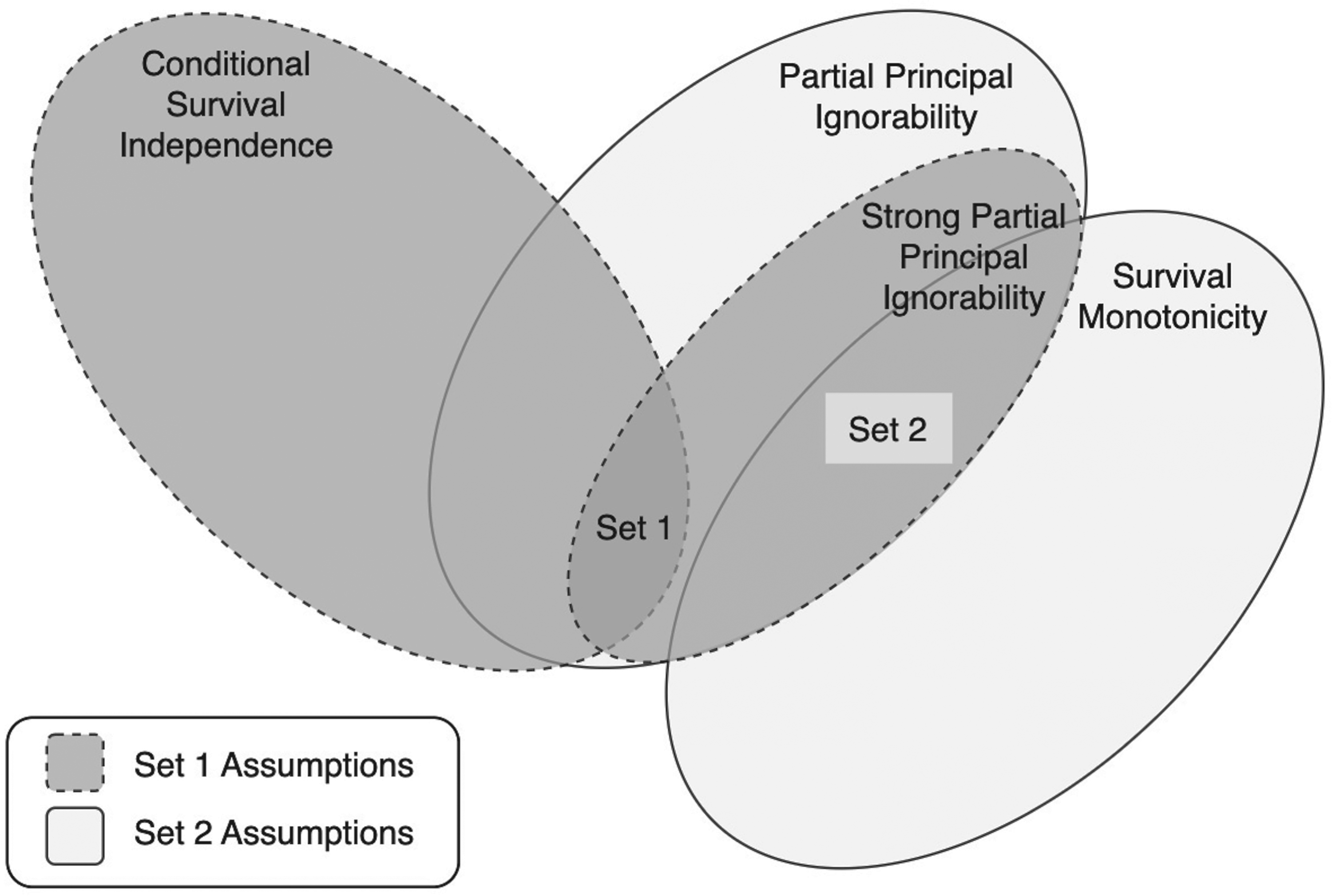
As we explain later, each set of assumptions motivate a distinct weighting estimator to identify SACE in CRTs. Given their seeming similarity to one another, it is important to conceptually distinguish between the Set 1 and Set 2 assumptions. We visualize their relationships in Figure 1, which is meant to demonstrate two salient features. First, S2A4 and S2A5 imply S1A5. For the case of $a=1$ , S2A5 directly implies S1A5, and for the case of $a=0$ , survival monotonicity, S2A4, means the event $S_{ij}(0)=1$ implies $S_{ij}(1)=1$ (i.e. a constant), which induces the stated conditional independence. ¹² Second, the Set 1 and Set 2 assumptions are mutually exclusive due to the relationship between S1A4 and S2A4. If S1A4 and S2A4 are simultaneously true, we would have for each individual and $X_i,C_i$ , $P(S_{ij}(1)=0,S_{ij}(0)=1|X_i,C_i)=P(S_{ij}(1)=0|X_i,C_i)P(S_{ij}(0)=1|X_i,C_i)=0$ , which is prohibited by the assumption of non-trivial survival, $0<P(S_{ij}(a)=1|X_i,C_i)<1$ , under $a=0,1$ . In summary, these two sets of assumptions live disjointly within the condition S1A5.

Figure 1.

Diagram of relationship between Set 1 and Set 2 assumptions for identification of SACE. Each assumption set is satisfied within the intersection of their respective conditions (where they are both preceded by Assumptions 1 to 3, non-trivial survival, and SUTVA). S1A4 $=$ conditional survival independence, S1A5 $=$ strong partial principal ignorability, S2A4 $=$ survival monotonicity, and S2A5 $=$ partial principal ignorability. SACE: survivor average causal effect; SUTVA: stable unit treatment value assumption.

The above framework puts forth the necessary causal assumptions for non-parametric identification supposing that we have a sufficient set of observed individual-level and cluster-level characteristics. However, in reality, even after conditioning on a rich set of baseline covariates, individuals’ outcomes within the same cluster tend to be positively correlated. If the source of this correlation is not accounted for in the assumptions, then the conditional independence statements of Set 1 (S1A4 and S1A5) and of Set 2 (S2A5), which hold across all individuals, may not be sufficiently strong to enable identification. To accommodate this complexity, we extend the above assumptions by having $C_i$ (wherever it appears) be comprised of two components, $C_i=(C_{i,\text{fe}}^T,b_i{)}^T$ where $C_{i,\text{fe}}$ denotes the component of $C_i$ whose values can be observed and $b_i$ , a parametric random intercept for cluster, which induces the within-cluster correlation. The caveat of this extension is that identification requires specification of the distributions of the latent variables $b_i$ and restricts the form of unmeasured confounding between survival and the final outcome. Similar latent cluster-level confounding assumptions have also been proposed in earlier work on clustered observational studies without truncation by death.^22,23 Specifically, as described in the next sections, we make a Gaussian specification for the $b_i$ enabling parametric survival status modeling according to conventional mixed effects logistic regression for binary survival status. Nevertheless, we also evaluate, using simulations, the consequence of ignoring the cluster-level random intercept for survival status modeling to generate practical recommendations.

2.2. Two identification formulas

We next present Identity 1 and Identity 2, which represent how SACE is point identified with estimable parameters with intuitive weighting under the Set 1 and Set 2 assumptions respectively. Importantly, for the two SACE quantities, any appearance of the non-mortal outcome will be predicated on survival (due to a product term). Interestingly, while different in form, they will both depend on the exact same models for survival status.

Identity 1. The parameters $\mu (a)$ for $a=0,1$ under Set 1 assumptions are identified with:

$$\mu (a)=\frac{E\{Y_{ij}I(A_i=a)S_{ij}{p}_{ij}^{1-a}(X_i,C_i)\}}{E\{I(A_i=a)S_{ij}{p}_{ij}^{1-a}(X_i,C_i)\}}$$

(3)

where $p_{ij}^{A_i}(X_i,C_i):=P(S_{ij}=1|A_i,X_i,C_i)$ . The weight $I(A_i=a)S_{ij}{p}_{ij}^{1-a}(X_i,C_i)$ means that the observed survivors within one treatment group are up-weighted by their probability of survival under the alternative treatment, which in turn signifies that individuals whose probability of being an always-survivor is higher are weighted more heavily. In the context of a CRT, the proof of Identity 1 is provided in Supplemental Material 1.1.

Identity 2. The parameters $\mu (a)$ under Set 2 assumptions are identified with:

$$\mu (0)=\frac{E\{Y_{ij}(1-A_i)S_{ij}\}}{E\{(1-A_i)S_{ij}\}}$$

(4)

and

$$\mu (1)=\frac{E\{Y_{ij}{A}_i{S}_{ij}{p}_{ij}^0(X_i,C_i)/p_{ij}^1(X_i,C_i)\}}{E\{A_i{S}_{ij}{p}_{ij}^0(X_i,C_i)/p_{ij}^1(X_i,C_i)\}}$$

(5)

By cluster-level SUTVA, S2A4, and $A_i\in \{0,1\}$ , we have $(1-A_i)S_{ij}=(1-A_i{)}^2{S}_{ij}(0)=(1-A_i)S_{ij}(0)S_{ij}(1)$ . Therefore, the weights of $\mu (0)$ are straightforward because those who are observed to have survived treatment 0 are always-survivors. The Set 2 assumptions also imply that $p_{ij}^0(X_i,C_i)=P(G_{ij}=(1,1)|X_i,C_i)$ . Since $p_{ij}^1(X_i,C_i)=P(G_{ij}=(1,1)|X_i,C_i)+P(G_{ij}=(1,0)|X_i,C_i)$ , the terms in $A_i{S}_{ij}{p}_{ij}^0(X_i,C_i)/p_{ij}^1(X_i,C_i)$ of $\mu (1)$ re-weight the observed survivors in the treated group, which are comprised of both always-survivors and protected patients, to reflect the population of always-survivors. In the context of a CRT, the proof of Identity 2 is presented in Supplemental Material 1.2.

It is critical to emphasize that the quantities, $\mu (a)$ , are expectations conditioned on $G_{ij}=(1,1)$ so, at the outset, it may seem as though the identified estimands would necessarily rely on models for $P(G_{ij}=g|X_i,C_i)$ with $g\in \{0,1\}\times \{0,1\}$ , referred to as “principal score models.” ¹¹ However, both the Set 1 and Set 2 assumptions, which contain cross-world conditions, allow for identification of $\mu (a)$ by separating the survival statuses and the non-mortal outcomes across treatments. As a result, we see that identification leads to products of survival status terms (as in equations (3) and (5) above)—one term that is observed and one that needs to be predicted given covariates and random effects under a given treatment. In contrast, the full likelihood based approaches, while avoiding these assumptions, require having to target the principal score models. From a practical point of view, modeling binary survival statuses is generally more straightforward than simultaneously modeling at least three principal strata.

2.3. Model specifications and weighting estimators

For our working survival modeling, we first consider that the data, $\{A_i,S_i,C_i,X_i\}$ , arise from each cluster independently. Given our beliefs about the mechanism of clustering effects, we will suppose that within each cluster $i$ , an individual’s survival status is drawn according to $S_{ij}|A_i,X_i,C_i;\gamma \sim \text{Bern}(\text{expit}\{D_{ij}^T\beta +b_i\})$ where $b_i\sim N(0,{\sigma }_b^2)$ with ${\sigma }_b^2>0$ , and $D_{ij}$ is a finite vector of observed regressors involving $A_i,X_i,C_{i,\text{fe}}$ . In practice, we often make a convenience choice that $D_{ij}=(1,A_i,X_{ij}^T,C_{i,\text{fe}}^T{)}^T$ such that the survival of each individual only depends on the characteristics of that individual but not those from other individuals in the same cluster (apart from shared cluster-level information). Therefore, for $a=0,1$ , each individual’s probability of survival is represented as follows:

$$p_{ij}^a(X_i,C_i;\gamma )=\frac{\exp \{D_{ij,a}^T\beta +b_i\}}{1+\exp \{D_{ij,a}^T\beta +b_i\}}$$

(6)

where $D_{ij,a}$ represents setting $A_i=a$ . The effect of treatment and observable baseline covariates on survival is captured in $\beta$ , and the unobserved effects of clustering on survival are represented via the random intercept $b_i$ with variance ${\sigma }_b^2$ , so that $\gamma =({\beta }^T,{\sigma }_b^2{)}^T$ is of finite dimension. Although we do not consider this possibility, $D_{ij}$ can also include treatment-by-covariate interactions as well as summary measures of individual-level covariates through $g(X_i)$ (e.g. ${\overline{X}}_i$ ) as in a contextual-effects model. ²⁴

Two common parametric approaches for analyzing survival status data from parallel-arm CRTs—that we will use for survival status modeling for our SACE estimators—are to (i) fit a GLMM, specifically a mixed effects logistic regression model with a random intercept for cluster membership and (ii) fit a GLM, specifically a logistic regression model (accounting for clustering only in the robust sandwich variance expression) where both models must include a treatment effect indicator. ¹³ Since the GLMM relies on modeling the distribution of survival status conditional on the random effects (as well as any observed covariates), it is referred to as a conditional model. In contrast, the GLM, for which no random effects are modeled, is referred to as a marginal model under working independence.

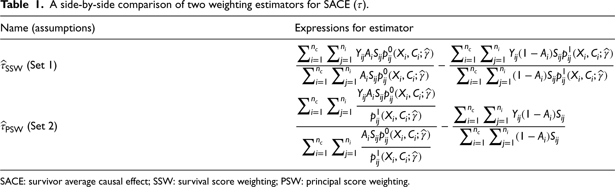
We will denote the estimators derived from Set 1 and Set 2, respectively, as the survival score weighting (SSW) estimator, ${\hat{\tau }}_{\text{SSW}}={\hat{\mu }}_{\text{SSW}}(1)-{\hat{\mu }}_{\text{SSW}}(0)$ , and the principal score weighting (PSW) estimator, ${\hat{\tau }}_{\text{PSW}}={\hat{\mu }}_{\text{PSW}}(1)-{\hat{\mu }}_{\text{PSW}}(0)$ . Their forms are summarized in Table 1. Although neither estimator fits principal scores directly, Set 2 uses that under monotonicity, the always-survivors principal stratum is comprised of exactly those that survive under treatment 0, whereas Set 1 relies on S1A4 breaking up the principal strata distributions (hence the naming convention). As discussed in Supplemental Material 1.3 and 1.4, ${\hat{\tau }}_{\text{SSW}}$ and ${\hat{\tau }}_{\text{PSW}}$ are consistent for SACE if ${\hat{\theta }}_{\text{SSW}}=({\hat{\gamma }}^T,{\hat{\mu }}_{\text{SSW}}(1),{\hat{\mu }}_{\text{SSW}}(0){)}^T$ and ${\hat{\theta }}_{\text{PSW}}=({\hat{\gamma }}^T,{\hat{\mu }}_{\text{PSW}}(1),{\hat{\mu }}_{\text{PSW}}(0){)}^T$ are a solution to unbiased estimating equations indexed by cluster, and if under the regularity conditions for which these ${\hat{\theta }}_{(\cdot )}\stackrel{p}{\to }{\theta }_0=({\gamma }_0^T,\mu (1),\mu (0){)}^T$ , we have correct specification of the working survival modeling such that ${\gamma }_0$ reflects the truth. ¹⁹ With latent cluster-level confounding, to achieve consistency, we would in principle fit the GLMM model (i) as it directly controls for $b_i$ as a random intercept.

Table 1.

A side-by-side comparison of two weighting estimators for SACE ( $\tau$ ).

Name (assumptions)	Expressions for estimator
${\hat{\tau }}_{\text{SSW}}$ (Set 1)	$\frac{{\displaystyle {\sum }_{i=1}^{n_c}{\sum }_{j=1}^{n_i}{Y}_{ij}{A}_i{S}_{ij}{p}_{ij}^0(X_i,C_i;\hat{\gamma })}}{{\displaystyle {\sum }_{i=1}^{n_c}{\sum }_{j=1}^{n_i}{A}_i{S}_{ij}{p}_{ij}^0(X_i,C_i;\hat{\gamma })}}-\frac{{\displaystyle {\sum }_{i=1}^{n_c}{\sum }_{j=1}^{n_i}{Y}_{ij}(1-A_i)S_{ij}{p}_{ij}^1(X_i,C_i;\hat{\gamma })}}{{\displaystyle {\sum }_{i=1}^{n_c}{\sum }_{j=1}^{n_i}(1-A_i)S_{ij}{p}_{ij}^1(X_i,C_i;\hat{\gamma })}}$
${\hat{\tau }}_{\text{PSW}}$ (Set 2)	$\frac{{\displaystyle {\sum }_{i=1}^{n_c}{\sum }_{j=1}^{n_i}\frac{Y_{ij}{A}_i{S}_{ij}{p}_{ij}^0(X_i,C_i;\hat{\gamma })}{p_{ij}^1(X_i,C_i;\hat{\gamma })}}}{{\displaystyle {\sum }_{i=1}^{n_c}{\sum }_{j=1}^{n_i}\frac{A_i{S}_{ij}{p}_{ij}^0(X_i,C_i;\hat{\gamma })}{p_{ij}^1(X_i,C_i;\hat{\gamma })}}}-\frac{{\displaystyle {\sum }_{i=1}^{n_c}{\sum }_{j=1}^{n_i}{Y}_{ij}(1-A_i)S_{ij}}}{{\displaystyle {\sum }_{i=1}^{n_c}{\sum }_{j=1}^{n_i}(1-A_i)S_{ij}}}$

SACE: survivor average causal effect; SSW: survival score weighting; PSW: principal score weighting.

According to the proposed identification assumptions, the marginal GLM model (ii), which assumes independence given observed covariates, is inherently mis-specified for predicting survival status. Only under the setting for which we are able to assume that there are absolutely no unobserved sources of within-cluster correlation of potential outcomes might this model be appropriate. Nonetheless, because cluster-indexed unbiased estimating equations are used to derive the GLM model parameters and SACE estimators, the asymptotic distribution of the SACE estimators have a sandwich variance, as demonstrated in Section 2.4 and in Supplemental Material 1.6, that can account for extra variation in the observed outcomes induced by clustering effects. Since the parameters of the survival status models themselves do not need to be interpreted, we juxtapose the small-sample performances of these two common modeling paradigms in the simulation study (Section 3) under data generation that explicitly includes a cluster-level random intercept as per the working model assumptions. Therefore, the marginal modeling strategy is considered in our simulations to elucidate the consequence of ignoring the latent cluster-level confounding under realistic levels of clustering observed in CRTs where intracluster correlation coefficients (ICCs) typically do not exceed 0.3. ²⁵

2.4. Variance estimation

In this section, we approximate the variance of the weighting estimators, ${\hat{\tau }}_{\text{SSW}}$ and ${\hat{\tau }}_{\text{PSW}}$ , by establishing their asymptotic distributions through the theory of M-estimation.^17–19 Our motivation for using asymptotic variance expressions stems from the limitations of the cluster bootstrap despite its conceptual simplicity. Specifically, cluster bootstrapping generally requires re-sampling entire clusters with replacement from the original data set to preserve the unknown within-cluster correlation structure, so it tends to work better for a large number of clusters. ²⁶ However, for even a moderate number of clusters, the computational time for the bootstrap approach with an acceptable number of replicates can be prohibitive since it requires fitting regression models repeatedly (such as generalized linear mixed model (GLMM)) to each bootstrapped data set. To this end, our proposed variance estimators serve as computationally efficient alternatives to re-sampling-based methods.

Recall we suppose that the available data $\{D_i,S_i,Y_i{\}}_{i=1}^{n_c}$ are mutually independent by cluster randomization (where the observable elements of $Y_i$ are for observed survivors). Suppose that each $D_{ij}$ and thus $\beta$ have dimension $p$ . Our focus is on the space of parameters of the form $\theta =({\gamma }^T,\mu (1),\mu (0){)}^T=({\beta }^T,{\sigma }_b^2,\mu (1),\mu (0){)}^T$ of dimension $(p+3)\times 1$ since our target estimand $\tau$ is simply the linear combination $k^T\theta$ , where $k=(0^T,0,1,-1{)}^T$ . For each $i$ , we define a function of observable data, $m(D_i,S_i,Y_i;\theta )=m_i(\theta )$ , which matches the dimension of $\theta$ , such that $E_{\theta }\{m_i(\theta )\}=0$ (for any $\theta$ ). Then, for the included number of clusters in the study $n_c$ , the solution to $\frac{1}{n_c}\sum _{i=1}^{n_c}{m}_i(\theta )=0$ is the M-estimator, $\hat{\theta }$ . However, since the identification of $\mu (1)$ and $\mu (0)$ are distinct for the Set 1 and Set 2 assumptions, the corresponding unbiased estimating equations must themselves be distinct with functions, $m_{\text{SSW},i}(\theta )$ and $m_{\text{PSW},i}(\theta )$ , and solutions, ${\hat{\theta }}_{\text{SSW}}$ and ${\hat{\theta }}_{\text{PSW}}$ .

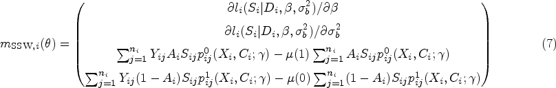
To obtain the unbiased estimating equations, we stack the score functions used to maximize the (marginalized) log-likelihood induced by the GLMM conditions, $l(S|D,\beta ,{\sigma }_b^2)=\sum _{i=1}^{n_c}{l}_i(S_i|D_i,\beta ,{\sigma }_b^2)$ (see Supplemental Material 1.4), which will be common to both the SSW and PSW estimators, and the functions that enable solving for ${\hat{\mu }}_{(\cdot )}(1)$ and ${\hat{\mu }}_{(\cdot )}(0)$ if the GLMM parameters, $\gamma$ , were known. The form of estimating functions corresponding to the Set 1 assumptions is

$$m_{\text{SSW},i}(\theta )=\left(\begin{array}{c}{\displaystyle \mathrm{\partial }{l}_i(S_i|D_i,\beta ,{\sigma }_b^2)/\mathrm{\partial }\beta }\\ {\displaystyle \mathrm{\partial }{l}_i(S_i|D_i,\beta ,{\sigma }_b^2)/\mathrm{\partial }{\sigma }_b^2}\\ \sum _{j=1}^{n_i}{Y}_{ij}{A}_i{S}_{ij}{p}_{ij}^0(X_i,C_i;\gamma )-\mu (1)\sum _{j=1}^{n_i}{A}_i{S}_{ij}{p}_{ij}^0(X_i,C_i;\gamma )\\ \sum _{j=1}^{n_i}{Y}_{ij}(1-A_i)S_{ij}{p}_{ij}^1(X_i,C_i;\gamma )-\mu (0)\sum _{j=1}^{n_i}(1-A_i)S_{ij}{p}_{ij}^1(X_i,C_i;\gamma )\end{array}\right)$$

(7)

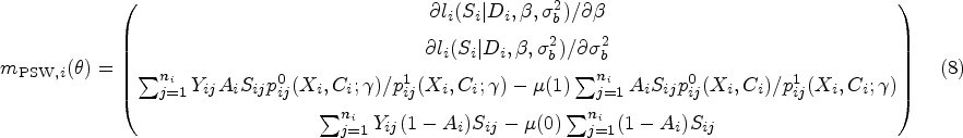
and for the Set 2 assumptions

$$m_{\text{PSW},i}(\theta )=\left(\begin{array}{c}\mathrm{\partial }{l}_i(S_i|D_i,\beta ,{\sigma }_b^2)/\mathrm{\partial }\beta \\ {\displaystyle \mathrm{\partial }{l}_i(S_i|D_i,\beta ,{\sigma }_b^2)/\mathrm{\partial }{\sigma }_b^2}\\ \sum _{j=1}^{n_i}{Y}_{ij}{A}_i{S}_{ij}{p}_{ij}^0(X_i,C_i;\gamma )/p_{ij}^1(X_i,C_i;\gamma )-\mu (1)\sum _{j=1}^{n_i}{A}_i{S}_{ij}{p}_{ij}^0(X_i,C_i)/p_{ij}^1(X_i,C_i;\gamma )\\ \sum _{j=1}^{n_i}{Y}_{ij}(1-A_i)S_{ij}-\mu (0)\sum _{j=1}^{n_i}(1-A_i)S_{ij}\end{array}\right)$$

(8)

Using first-order Taylor approximations coupled with certain regularity conditions for these independent data, applications of Slutsky’s and continuous mapping theorems give us that $\sqrt{n_c}({\hat{\tau }}_{\text{SSW}}-{\tau }_0)$ and $\sqrt{n_c}({\hat{\tau }}_{\text{PSW}}-{\tau }_0)$ converge in distribution to $N(0,k^T{V}_{{\theta }_0}k)$ . ¹⁹ Under correct specification, ${\tau }_0$ and ${\theta }_0$ are the true parameters, and $V_{{\theta }_0}$ is the true asymptotic variance as written out in Supplemental Material 1.3 (equation (20)). Note, we only subscript estimators with SSW and PSW and not parameters because parameters cannot be simultaneously identified under Set 1 and Set 2. The form of the estimator of the asymptotic variance, often termed a cluster-robust sandwich variance estimator, is

$${\hat{V}}_{{\hat{\theta }}_{(\cdot )}}={\left[\frac{1}{n_c}\sum _{i=1}^{n_c}\left\{\frac{\mathrm{\partial }{m}_{(\cdot ),i}({\hat{\theta }}_{(\cdot )})}{\mathrm{\partial }{\theta }^T}\right\}\right]}^{-1}\frac{1}{n_c}\sum _{i=1}^{n_c}{m}_{(\cdot ),i}({\hat{\theta }}_{(\cdot )})m_{(\cdot ),i}({\hat{\theta }}_{(\cdot )}{)}^T{\left[\frac{1}{n_c}\sum _{i=1}^{n_c}\left\{\frac{\mathrm{\partial }{m}_{(\cdot ),i}({\hat{\theta }}_{(\cdot )})}{\mathrm{\partial }{\theta }^T}\right\}\right]}^{-T}$$

(9)

The regularity conditions under which ${\hat{V}}_{{\hat{\theta }}_{(\cdot )}}$ is consistent for $V_{{\theta }_0}$ are posited by Iverson and Randles. ²⁷ The full expressions for the estimating functions (including the derivative of the log-likelihood) and a more thorough sketch of the asymptotic arguments are in Supplemental Material 1.3 and 1.4.

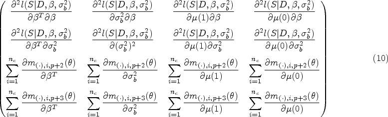
Now, we must determine the components of the sandwich variance for each estimator. We denote the middle matrices with $M_{\text{SSW}}(\theta )=\sum _{i=1}^{n_c}{m}_{\text{SSW},i}(\theta )m_{\text{SSW},i}(\theta {)}^T$ and $M_{\text{PSW}}(\theta )=\sum _{i=1}^{n_c}{m}_{\text{PSW},i}(\theta )m_{\text{PSW},i}(\theta {)}^T$ . The estimating functions that are required to find the middle matrices are already written above. We must also find the outer matrices, which we will denote by $B_{\text{SSW}}(\theta )=\sum _{i=i}^{n_c}\mathrm{\partial }{m}_{\text{SSW},i}(\theta )/\mathrm{\partial }{\theta }^T$ and $B_{\text{PSW}}(\theta )=\sum _{i=i}^{n_c}\mathrm{\partial }{m}_{\text{PSW},i}(\theta )/\mathrm{\partial }{\theta }^T$ . The general form of the outer matrices, $B_{(\cdot )}(\theta )$ , is

$$\begin{array}{r}\left(\begin{array}{cccc}{\displaystyle \frac{{\mathrm{\partial }}^{2}l(S|D,\beta ,{\sigma }_b^2)}{\mathrm{\partial }{\beta }^T\mathrm{\partial }\beta }}& {\displaystyle \frac{{\mathrm{\partial }}^{2}l(S|D,\beta ,{\sigma }_b^2)}{\mathrm{\partial }{\sigma }_b^2\mathrm{\partial }\beta }}& {\displaystyle \frac{{\mathrm{\partial }}^{2}l(S|D,\beta ,{\sigma }_b^2)}{\mathrm{\partial }\mu (1)\mathrm{\partial }\beta }}& {\displaystyle \frac{{\mathrm{\partial }}^{2}l(S|D,\beta ,{\sigma }_b^2)}{\mathrm{\partial }\mu (0)\mathrm{\partial }\beta }}\\ {\displaystyle \frac{{\mathrm{\partial }}^{2}l(S|D,\beta ,{\sigma }_b^2)}{\mathrm{\partial }{\beta }^T\mathrm{\partial }{\sigma }_b^2}}& {\displaystyle \frac{{\mathrm{\partial }}^{2}l(S|D,\beta ,{\sigma }_b^2)}{\mathrm{\partial }({\sigma }_b^2{)}^2}}& {\displaystyle \frac{{\mathrm{\partial }}^{2}l(S|D,\beta ,{\sigma }_b^2)}{\mathrm{\partial }\mu (1)\mathrm{\partial }{\sigma }_b^2}}& {\displaystyle \frac{{\mathrm{\partial }}^{2}l(S|D,\beta ,{\sigma }_b^2)}{\mathrm{\partial }\mu (0)\mathrm{\partial }{\sigma }_b^2}}\\ {\displaystyle \sum _{i=1}^{n_c}\frac{\mathrm{\partial }{m}_{(\cdot ),i,p+2}(\theta )}{\mathrm{\partial }{\beta }^T}}& {\displaystyle \sum _{i=1}^{n_c}\frac{\mathrm{\partial }{m}_{(\cdot ),i,p+2}(\theta )}{\mathrm{\partial }{\sigma }_b^2}}& {\displaystyle \sum _{i=1}^{n_c}\frac{\mathrm{\partial }{m}_{(\cdot ),i,p+2}(\theta )}{\mathrm{\partial }\mu (1)}}& {\displaystyle \sum _{i=1}^{n_c}\frac{\mathrm{\partial }{m}_{(\cdot ),i,p+2}(\theta )}{\mathrm{\partial }\mu (0)}}\\ {\displaystyle \sum _{i=1}^{n_c}\frac{\mathrm{\partial }{m}_{(\cdot ),i,p+3}(\theta )}{\mathrm{\partial }{\beta }^T}}& {\displaystyle \sum _{i=1}^{n_c}\frac{\mathrm{\partial }{m}_{(\cdot ),i,p+3}(\theta )}{\mathrm{\partial }{\sigma }_b^2}}& {\displaystyle \sum _{i=1}^{n_c}\frac{\mathrm{\partial }{m}_{(\cdot ),i,p+3}(\theta )}{\mathrm{\partial }\mu (1)}}& {\displaystyle \sum _{i=1}^{n_c}\frac{\mathrm{\partial }{m}_{(\cdot ),i,p+3}(\theta )}{\mathrm{\partial }\mu (0)}}\end{array}\right)\end{array}$$

(10)

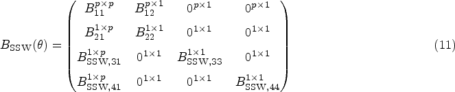
where the third index of $m_{(\cdot ),i,k}(\theta )$ represents the $k$ -th component of the $i$ -th vector function. Due to the nature of the stacked estimating equations, for which the score equations are solved independently, we have matrix structures $B_{\text{SSW}}(\theta )$ and $B_{\text{PSW}}(\theta )$ that are relatively sparse. However, they have different forms since $\mu (0)$ under the Set 2 assumptions is not identified with a parameter that involves a model for survival events. For the SSW estimator, we have outer matrix:

$$B_{\text{SSW}}(\theta )=\left(\begin{array}{cccc}{B}_{11}^{p\times p}& B_{12}^{p\times 1}& 0^{p\times 1}& 0^{p\times 1}\\ B_{21}^{1\times p}& B_{22}^{1\times 1}& 0^{1\times 1}& 0^{1\times 1}\\ B_{\text{SSW},31}^{1\times p}& 0^{1\times 1}& B_{\text{SSW},33}^{1\times 1}& 0^{1\times 1}\\ B_{\text{SSW},41}^{1\times p}& 0^{1\times 1}& 0^{1\times 1}& B_{\text{SSW},44}^{1\times 1}\end{array}\right)$$

(11)

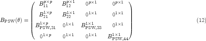
for the PSW estimator,

$$\begin{array}{r}{B}_{\text{PSW}}(\theta )=\left(\begin{array}{cccc}{B}_{11}^{p\times p}& B_{12}^{p\times 1}& 0^{p\times 1}& 0^{p\times 1}\\ B_{21}^{1\times p}& B_{22}^{1\times 1}& 0^{1\times 1}& 0^{1\times 1}\\ B_{\text{PSW},31}^{1\times p}& 0^{1\times 1}& B_{\text{PSW},33}^{1\times 1}& 0^{1\times 1}\\ 0^{1\times p}& 0^{1\times 1}& 0^{1\times 1}& B_{\text{PSW},44}^{1\times 1}\end{array}\right)\end{array}$$

(12)

where the superscripts denote the dimension of the submatrices ( $\theta$ on the RHS is suppressed for notation simplicity). Using the estimator of the asymptotic variance as in equation (9), we can approximate the variances for the SACE estimators, ${\hat{\tau }}_{\text{SSW}}$ and ${\hat{\tau }}_{\text{PSW}}$ , with $k^T{B}_{\text{SSW}}({\hat{\theta }}_{\text{SSW}}{)}^{-1}{M}_{\text{SSW}}({\hat{\theta }}_{\text{SSW}})B_{\text{SSW}}({\hat{\theta }}_{\text{SSW}}{)}^{-T}k$ and $k^T{B}_{\text{PSW}}({\hat{\theta }}_{\text{PSW}}{)}^{-1}{M}_{\text{PSW}}({\hat{\theta }}_{\text{PSW}})B_{\text{PSW}}({\hat{\theta }}_{\text{PSW}}{)}^{-T}k$ , respectively. These expressions assume that $B_{\text{SSW}}({\hat{\theta }}_{\text{SSW}})$ and $B_{\text{PSW}}({\hat{\theta }}_{\text{PSW}})$ are non-singular, which will generally be the case for a sufficiently large sample of clusters. Each non-zero entry of $B_{\text{SSW}}(\theta )$ and $B_{\text{PSW}}(\theta )$ is fully written out in Supplemental Material 1.4. Estimates of the GLMM parameters can be obtained from standard statistical software. However, both the outer and middle matrices involve integrals, as a byproduct of marginalizing over the random intercept in the likelihood, that are not solvable analytically. Computing these integrals numerically is not a trivial exercise as shown in prior work. ²⁸ Since the entries in the matrices are complex (particularly in the outer matrix), just keeping track of the integral expressions and ensuring that they are numerically integrable is a cumbersome task. After accounting for these integrals, we employ a numerical integration technique that is well-suited to integrals representing Gaussian expectations. In the Supplemental Material 1.5, we present all integrals involved in variance estimation as well as outline our choice and usage of adaptive Gauss-Hermite quadrature (AGQ) ²⁹ for the required numerical integration. Despite the necessity of said numerical methods, for the cases in our simulation study where the non-parametric cluster bootstrap is viable, the variance estimates using the asymptotic distributions are not meaningfully different than those using the bootstrap but the computation times are reduced substantially (for reference, see Table S4 of Supplemental Material 2).

The process for determining asymptotic distributions under the GLMM for survival status requires a similar formulation to the above, but the random intercept terms and row for ${\sigma }_b^2$ are removed from the estimating functions as outlined in Supplemental Material 1.6; accordingly, no numerical integration is required for estimation. Therefore, for clarity of notation, we will henceforth distinguish the SACE estimated using the GLM from the GLMM by using parameter estimators denoted with a tilde, which so far include $\tilde{\beta }$ , ${\tilde{\theta }}_{\text{SSW}}$ , ${\tilde{\mu }}_{\text{SSW}}(a)$ , ${\tilde{\tau }}_{\text{SSW}}$ , ${\tilde{\theta }}_{\text{PSW}}$ , ${\tilde{\mu }}_{\text{PSW}}(a)$ , and ${\tilde{\tau }}_{\text{PSW}}$ for $a=0,1$ . We note that Table 1 omits this notational distinction for continuity and succinctness. Since the parameter estimates for SACE are conceived as solutions to estimating equations that sum with respect to the cluster index, we obtain a sandwich variance expression that accounts for clustering when using the GLM. More specifically, the analogous sub-matrix of $B_{(\cdot )}({\tilde{\theta }}_{(\cdot )}{)}^{-1}{M}_{(\cdot )}({\tilde{\theta }}_{(\cdot )})B_{(\cdot )}({\tilde{\theta }}_{(\cdot )}{)}^{-T}$ corresponding to the estimated variance matrix for the model coefficients is precisely the sandwich variance estimate that we would achieve by solving a GEE ³⁰ with mean and variance models as in logistic regression with a working correlation matrix for independence (Supplemental Material 1.6). In terms of interpretation and estimation, solving GEEs (marginal) are often compared to and viewed as a standard alternative to fitting GLMMs (conditional).^13,31 Although in this setting the parameters of the survival status models are not of interest, we emphasize that marginal and conditional logistic regression models are separate conceptual frameworks, whose parameters do not necessarily coincide (due to a lack of collapsibility). ³² As it pertains to inference, these two approaches may also perform differently with CRTs for a binary response depending on the study conditions, for example, the number of clusters and the strength of the within-cluster correlation, ³³ and we compare the effect of these modeling choices for SACE estimation across various scenarios in the simulation study in Section 3.

There are well-documented issues with small-sample inference associated with sandwich variance estimators, either from marginal or conditional modeling, for the analysis of CRTs. These estimators tend to underestimate the true variance in small samples and lead to anticonservative inference.^34,35 As such, we suggest employing a bias-corrected version of the proposed sandwich variance estimators (whether or not conditioning on random effects). For our simulation study and data application, we use a simple degrees of freedom correction, ³⁶ multiplying the variance terms by $n_c/(n_c-\mathrm{\#}\text{params})$ , where “params” refers to all survival status model parameters as well as $\mu (1)$ and $\mu (0)$ ; note, for the GLMM, we have one additional parameter for the random effect variance. While this proved sufficient for achieving near nominal coverage in our simulations and thus suitable to our motivating application, alternative corrections to the sandwich variance estimates may warrant future research.

Lastly, it may be that for the fitted GLMM, ${\sigma }_b^2$ is estimated to be 0 when using statistical software. This estimate arises due to the fact that convergence to a maximum is restricted by the boundary condition on the parameter space, where the variance of the random intercept must be at least 0; for further treatment of this phenomenon including asymptotics, see Self and Liang. ³⁷ Therefore, constrained optimization algorithms will permit estimates of 0 for the variance, which is the default for the prevailing GLMM fitting package lme4 in R. ³⁸ When this phenomenon occurs, it produces (virtually) the same coefficient estimates as the GLM, and thus can be constructed as the solution to the corresponding estimating equations (i.e. those which drop the random intercept); nonetheless, we treat it as a separate case from the marginal model approach because we penalize for the extra variance parameter. There are options to explicitly avoid a zero variance estimate such as changing the optimizer or putting a prior on the variance parameter that pulls it away from 0, ³⁹ but we adopt the most standard application of the existing R software allowing for a zero variance component estimate.

3. Simulation study

In our simulation study, we assess the performance of the SACE estimators under different data generating mechanisms. We follow the ADEMP (Aims, Data-generating mechanisms, Methods, Estimands, Performance measures) schema defined by Morris et al. ⁴⁰ to describe our simulation study. There are two primary goals for these simulations. The first goal is to evaluate the two weighting SACE estimators when the data generation adheres to either the Set 1 assumptions or the Set 2 assumptions in terms of their empirical bias and coverage (see Section 3.2 for more details). We recall that these are technically mutually exclusive data generating mechanisms because S1A4, conditional survival independence, and S2A4, the deterministic requirement of survival monotonicity, cannot exist simultaneously. Because of S1A4, it is natural to define a data generating mechanism that adheres to the Set 1 assumptions but operates on the survival terms separately. For the Set 2 assumptions, we follow the approach of Jiang et al. ⁴¹ by imposing stochastic monotonicity, ⁴² where we make the probability of survival under treatment $a=1$ greater than under treatment $a=0$ conditional on covariates. For our simulation, we increase the magnitude of the treatment effect on survival substantially so as to drive the empirical incidence of harmed patients to near 0. Of note, it is also possible to simulate data which achieves deterministic survival monotonicity and maintains the target marginal survival status models by specifying models for $S_{ij}(1)$ given values of $S_{ij}(0)$ . ⁴³ This approach is also equivalent to an ordinal representation of the principal strata model, where stratum membership is assigned by thresholding a latent continuous response variable with cut-points that represent the treatment effect on survival, but such ordering of stratum membership is not intrinsic. The results for this ordinal approach as presented in Table S3 (Supplemental Material 2) are consistent relative to the other data generating mechanisms, so we save this exploration for Supplemental Material 1.7.

The second aim is to evaluate how well our SACE estimators handle latent clustering effects, represented by unobserved cluster-level random intercepts in the data generating process for the mortality and non-mortality outcomes. To this end, we compare the performance of the estimators with GLMM survival status modeling, ${\hat{\tau }}_{\text{SSW}}$ and ${\hat{\tau }}_{\text{PSW}}$ , to those with GLM survival status modeling (with cluster-robust variance), ${\tilde{\tau }}_{\text{SSW}}$ and ${\tilde{\tau }}_{\text{PSW}}$ . Variance expressions and confidence $z$ -intervals are computed based on the asymptotic distributions discussed in Section 2 and in Supplemental Material 1.

3.1. Data generating process

We consider scenarios for which we choose the number of clusters $n_c\in \{30,60,90\}$ . The number of individuals in each cluster is drawn from a discrete uniform distribution, $n_i\sim \text{Unif}\{25,50\}$ . We generate two individual-level covariates for each cluster, $X_{i,1}\sim {\text{MVN}}_{n_i}(\mathbf{2},0.5I_{n_i})$ and $X_{i,2}\sim {\text{MVN}}_{n_i}(\mathbf{0.5},0.25I_{n_i})$ and one cluster-level covariate, $C_{i,1}\sim \text{Bern}(0.3)$ . We incorporate latent cluster-level effects via the variables $b_i$ and $b_i^{*}$ for survival status and the non-mortal outcome respectively, where we suppose $b_i^{*}\sim N(0,1/9)$ and $b_i=\xi b_i^{*}$ ; given $\xi >0$ , we see that this setup induces a source of unobservable correlation between individuals’ non-mortal and survival events within each cluster. These variables differ from the observed covariates because we only propose their distributional form and relationship to other variables, but their actual values are unknown to us. For $a=0,1$ , we generate survival status and non-mortal outcomes according to:

$$\begin{array}{rl}& S_{ij}(a)|X_{ij},C_{i,1},b_i\sim \text{Bern}(\text{expit}\{0.75+\delta a+0.1X_{ij,1}-0.05X_{ij,2}+0.1C_{i,1}+b_i\})\end{array}$$

(13)

$$\begin{array}{rl}& Y_{ij}(a)|S_{ij}(a)=1,X_{ij},C_{i,1},b_i^{*}\sim \text{N}((a+1)(1+0.25X_{ij,1}+0.125X_{ij,2})+b_i^{*},1)\end{array}$$

(14)

For treatment effect, we consider $\delta \in \{0,\log (1.25),\log (5)\}$ . The values of $0$ and $\log (1.25)$ represent Set 1 data generation and $\log (5)$ represents Set 2 data generation because the treatment effect is large enough to induce near empirical monotonicity.

We quantify the strength of the latent clustering effects for each data generating mechanism via the ICC. For the continuous non-mortal outcomes, the ICC or equivalently the correlation among individuals within the same cluster is given by $\rho ={\sigma }_{b^{*}}^2/({\sigma }_{b^{*}}^2+{\sigma }_{ϵ}^2)$ , which is set equal to $0.1$ . We define the ICC for survival as $\lambda ={\sigma }_b^2/({\sigma }_b^2+{\pi }^2/3)$ . This standard representation for ICC for mixed effects logistic regression is motivated via a latent variable model, which creates a dichotomous outcome by thresholding an underlying continuous variable with a standard logistic distribution.^44,45 We briefly show how it is derived as a note in Supplemental Material 1.7. This definition of the ICC for GLMMs then allows for an analogous interpretation to the ICC for linear mixed models (LMMs), except that it is defined on the latent or log-odds scale. Since $b_i\sim N(0,{\xi }^2{\sigma }_{b^{*}}^2)$ , we choose values of $\xi$ such that $\lambda ={\xi }^2{\sigma }_{b^{*}}^2/({\xi }^2{\sigma }_{b^{*}}^2+{\pi }^2/3)\in \{0.3,0.1\}$ .

For finding the true parameters, we generate the data using a large number of clusters, $n_c=1000$ , as if to represent the population of clusters. We define the true SACE estimand within each simulation as

$$\frac{\sum _{i=1}^{1000}\sum _{j=1}^{n_i}{Y}_{ij}(1)S_{ij}(0)S_{ij}(1)}{\sum _{i=1}^{1000}\sum _{j=1}^{n_i}{S}_{ij}(0)S_{ij}(1)}-\frac{\sum _{i=1}^{1000}\sum _{j=1}^{n_i}{Y}_{ij}(0)S_{ij}(0)S_{ij}(1)}{\sum _{i=1}^{1000}\sum _{j=1}^{n_i}{S}_{ij}(0)S_{ij}(1)}$$

(15)

For the results presented in the next section, the percentage of always-survivors under $n_c=1000$ ranges from $51\mathrm{\%}$ to $65\mathrm{\%}$ , where larger values of $\delta$ and smaller $\lambda$ induce higher rates of this subgroup.

For each data generating mechanism, the observed data are obtained after random allocation of clusters to treatment where $A_i\sim \text{Bern}(0.5)$ . For example, if cluster $i$ is assigned to treatment 1, the observed data are $\{Y_i(1),S_i(1),X_i,C_{i,1}\}$ with cluster size $n_i$ . In the next section, we report the performance of SACE estimates on these observed data under the different data generation assumptions and modeling techniques as described above. The results for the additional values of $\delta =-\log (1.25)$ and $\lambda \in \{0.15,0.05\}$ as well as the scenarios for deterministic monotonicity are presented in Supplemental Material 2.

3.2. Simulation results

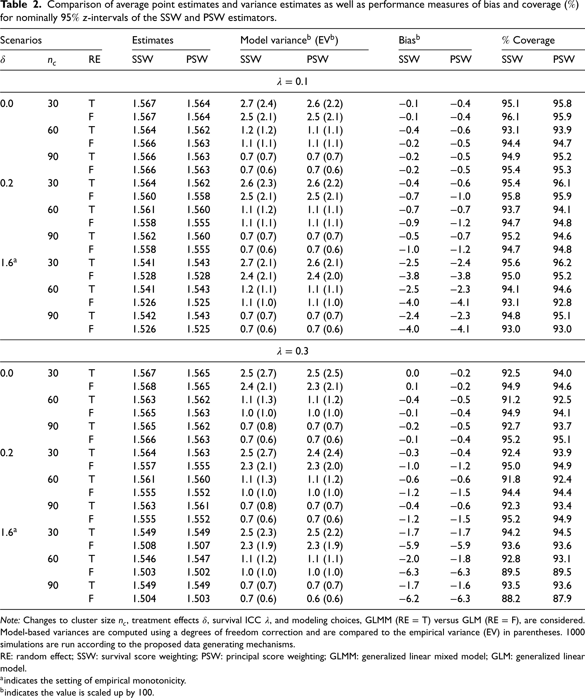
We include four measures to evaluate the performance of the estimators under the various simulation scenarios: empirical bias, empirical variance, average of the estimated variance, and coverage of the $95\mathrm{\%}$ confidence interval. The empirical or Monte Carlo variance is included in parentheses as a benchmark for the average of the estimated variance. Results for 1000 simulations are presented in Table 2, where the bias and variance metrics are scaled by 100.

Table 2.

Comparison of average point estimates and variance estimates as well as performance measures of bias and coverage ( $\mathrm{\%}$ ) for nominally $95\mathrm{\%}$ $z$ -intervals of the SSW and PSW estimators.

Scenarios			Estimates		Model variance ${}^{\mathrm{b}}$ (EV ${}^{\mathrm{b}}$ )		Bias ${}^{\mathrm{b}}$		$\mathrm{\%}$ Coverage
$\delta$	$n_c$	RE	SSW	PSW	SSW	PSW	SSW	PSW	SSW	PSW
$\lambda =0.1$
0.0	30	T	1.567	1.564	2.7 (2.4)	2.6 (2.2)	−0.1	−0.4	95.1	95.8
		F	1.567	1.564	2.5 (2.1)	2.5 (2.1)	−0.1	−0.4	96.1	95.9
	60	T	1.564	1.562	1.2 (1.2)	1.1 (1.1)	−0.4	−0.6	93.1	93.9
		F	1.566	1.563	1.1 (1.1)	1.1 (1.1)	−0.2	−0.5	94.4	94.7
	90	T	1.566	1.563	0.7 (0.7)	0.7 (0.7)	−0.2	−0.5	94.9	95.2
		F	1.566	1.563	0.7 (0.6)	0.7 (0.6)	−0.2	−0.5	95.4	95.3
0.2	30	T	1.564	1.562	2.6 (2.3)	2.6 (2.2)	−0.4	−0.6	95.4	96.1
		F	1.560	1.558	2.5 (2.1)	2.5 (2.1)	−0.7	−1.0	95.8	95.9
	60	T	1.561	1.560	1.1 (1.2)	1.1 (1.1)	−0.7	−0.7	93.7	94.1
		F	1.558	1.555	1.1 (1.1)	1.1 (1.1)	−0.9	−1.2	94.7	94.8
	90	T	1.562	1.560	0.7 (0.7)	0.7 (0.7)	−0.5	−0.7	95.2	94.6
		F	1.558	1.555	0.7 (0.6)	0.7 (0.6)	−1.0	−1.2	94.7	94.8
1.6 ${}^{\mathrm{a}}$	30	T	1.541	1.543	2.7 (2.1)	2.6 (2.1)	−2.5	−2.4	95.6	96.2
		F	1.528	1.528	2.4 (2.1)	2.4 (2.0)	−3.8	−3.8	95.0	95.2
	60	T	1.541	1.543	1.2 (1.1)	1.1 (1.1)	−2.5	−2.3	94.1	94.6
		F	1.526	1.525	1.1 (1.0)	1.1 (1.0)	−4.0	−4.1	93.1	92.8
	90	T	1.542	1.543	0.7 (0.7)	0.7 (0.7)	−2.4	−2.3	94.8	95.1
		F	1.526	1.525	0.7 (0.6)	0.7 (0.6)	−4.0	−4.1	93.0	93.0
$\lambda =0.3$
0.0	30	T	1.567	1.565	2.5 (2.7)	2.5 (2.5)	0.0	−0.2	92.5	94.0
		F	1.568	1.565	2.4 (2.1)	2.3 (2.1)	0.1	−0.2	94.9	94.6
	60	T	1.563	1.562	1.1 (1.3)	1.1 (1.2)	−0.4	−0.5	91.2	92.5
		F	1.565	1.563	1.0 (1.0)	1.0 (1.0)	−0.1	−0.4	94.9	94.1
	90	T	1.565	1.562	0.7 (0.8)	0.7 (0.7)	−0.2	−0.5	92.7	93.7
		F	1.566	1.563	0.7 (0.6)	0.7 (0.6)	−0.1	−0.4	95.2	95.1
0.2	30	T	1.564	1.563	2.5 (2.7)	2.4 (2.4)	−0.3	−0.4	92.4	93.9
		F	1.557	1.555	2.3 (2.1)	2.3 (2.0)	−1.0	−1.2	95.0	94.9
	60	T	1.561	1.560	1.1 (1.3)	1.1 (1.2)	−0.6	−0.6	91.8	92.4
		F	1.555	1.552	1.0 (1.0)	1.0 (1.0)	−1.2	−1.5	94.4	94.4
	90	T	1.563	1.561	0.7 (0.8)	0.7 (0.7)	−0.4	−0.6	92.3	93.4
		F	1.555	1.552	0.7 (0.6)	0.7 (0.6)	−1.2	−1.5	95.2	94.9
1.6 ${}^{\mathrm{a}}$	30	T	1.549	1.549	2.5 (2.3)	2.5 (2.2)	−1.7	−1.7	94.2	94.5
		F	1.508	1.507	2.3 (1.9)	2.3 (1.9)	−5.9	−5.9	93.6	93.6
	60	T	1.546	1.547	1.1 (1.2)	1.1 (1.1)	−2.0	−1.8	92.8	93.1
		F	1.503	1.502	1.0 (1.0)	1.0 (1.0)	−6.3	−6.3	89.5	89.5
	90	T	1.549	1.549	0.7 (0.7)	0.7 (0.7)	−1.7	−1.6	93.5	93.6
		F	1.504	1.503	0.7 (0.6)	0.6 (0.6)	−6.2	−6.3	88.2	87.9

Note: Changes to cluster size $n_c$ , treatment effects $\delta$ , survival ICC $\lambda$ , and modeling choices, GLMM (RE = T) versus GLM (RE = F), are considered. Model-based variances are computed using a degrees of freedom correction and are compared to the empirical variance (EV) in parentheses. 1000 simulations are run according to the proposed data generating mechanisms.

RE: random effect; SSW: survival score weighting; PSW: principal score weighting; GLMM: generalized linear mixed model; GLM: generalized linear model.

${}^{\mathrm{a}}$ indicates the setting of empirical monotonicity.

${}^{\mathrm{b}}$ indicates the value is scaled up by $100$ .

Overall, the simulation study reveals that both of the proposed SACE estimators, where the mortality outcome is modeled using mixed effects logistic regression, exhibit low bias across all data generating scenarios. The $95\mathrm{\%}$ $z$ -intervals constructed using the asymptotic variance expressions with a degrees of freedom adjustment in general get close to nominal rates. In summary, regardless of the assumptions underlying the data generating mechanism, ${\hat{\tau }}_{\text{SSW}}$ and ${\hat{\tau }}_{\text{PSW}}$ tend to perform similarly and well, where there may be a slight advantage to the latter estimator. This empirically shows that ${\hat{\tau }}_{\text{SSW}}$ and ${\hat{\tau }}_{\text{PSW}}$ are relatively robust to certain departures from their requisite identification assumptions in CRT settings, that is, when the identification assumptions underlying the other estimator hold and when data generating process mimics realistic CRTs. Performance instead appears to be most affected by modeling choice, where we see analogous patterns for the SSW and PSW estimators.

The results demonstrate that there is usually benefit relative to bias for explicitly accounting for clustering effects in modeling the mortality event via a GLMM as opposed to a GLM. The differences in their bias are relatively negligible in most scenarios, but the bias of ${\tilde{\tau }}_{\text{SSW}}$ and ${\tilde{\tau }}_{\text{PSW}}$ becomes more pronounced when the treatment effect on survival status further deviates from zero. In general, the fixed effects parameters in marginal logistic models tend to be attenuated towards zero, ⁴⁶ which accords with the opposite sign bias we see with the GLM when there are larger treatment effects. For the most part, when there are small treatment effects, the coverage rates are comparable across these modeling techniques, and they all are near to the nominal $95\mathrm{\%}$ rate. However, when the value of $\lambda$ is higher, such as 0.3 (and occasionally 0.15), the constructed confidence intervals for ${\hat{\tau }}_{\text{SSW}}$ and ${\hat{\tau }}_{\text{PSW}}$ tend to suffer from undercoverage as compared ${\tilde{\tau }}_{\text{SSW}}$ and ${\tilde{\tau }}_{\text{PSW}}$ even though the variance estimates of the former are higher on average (regardless of small-sample corrections). Discrepancies here might be explained by the inferential trade-offs of using a marginal model in lieu of a conditional model in the presence of certain values of ICC.^13,33,47,48 Given our observations in the small treatment effect scenarios, opting for ${\tilde{\tau }}_{\text{SSW}}$ and ${\tilde{\tau }}_{\text{PSW}}$ may suffice even if they cost some in terms of bias. However, the story for inference is different when the treatment effect on survival is large, particularly for higher values of $\lambda$ . The interval estimates for ${\hat{\tau }}_{\text{SSW}}$ and ${\hat{\tau }}_{\text{PSW}}$ achieve closer to nominal coverage as opposed to ${\tilde{\tau }}_{\text{SSW}}$ and ${\tilde{\tau }}_{\text{PSW}}$ , which demonstrate noticeable undercoverage. In our simulations, all of the average estimated variances are close to their empirical counterparts signifying that our variance estimators perform adequately in finite samples, and bias, particularly for the GLM, is mostly driving the coverage results. The results for additional treatment effects and survival ICC are shown in Tables S1 to S3 of Supplemental Material 2 and in general are consistent with those presented above.

In selected scenarios, we have also examined the performance of the cluster bootstrap for generating variance estimates and confidence intervals, presented in Table S4 of Supplemental Material 2. We observe that the results are similar (if not slightly worse in terms of coverage) to the proposed variance estimators. However, the computation time required by our variance estimators is on average reduced by more than 10-fold for GLMM modeling and more than 60-fold for GLM modeling relative to the corresponding non-parametric bootstrap methods with 250 replicates.

4. Application to the RESTORE trial

We apply the weighting methods to estimate SACE in the Randomized Evaluation of Sedation Titration for Respiratory Failure (RESTORE) trial, a CRT investigating the effect of protocolized sedation on mechanical ventilation for children with acute respiratory failure, first analyzed by Curley et al. ⁴⁹ In this study, 31 pediatric intensive care units (PICUs) were randomized in parallel to one of two treatment arms pertaining to sedation practices. Following the necessary training, intervention PICUs (17 sites) managed sedation according to a goal-directed nurse-implemented comfort algorithm informed by illness trajectory, pain and arousal assessments, extubation readiness testing, sedation reevaluation every 8 hours, and weaning status. Control PICUs (14 sites) administered sedation per their usual care and in the absence of a protocol. The cluster sizes range from 12 to 272 with a median size of 57, and there are a total of 2449 children with 1225 in intervention and 1224 in control. There are 110 (4.5 $\mathrm{\%}$ ) observed deaths of which 47 (3.8 $\mathrm{\%}$ ) are in the intervention group and 63 (5.1 $\mathrm{\%}$ ) are in the control group.

In our analysis of RESTORE, the non-mortal outcome of interest is duration in days on a mechanical ventilator for a 28-day period. Duration on a ventilator not only has potential implications for the length of convalescence and overall health and well-being of a patient but may also impact resource availability in healthcare systems. ⁵⁰ Patients who do not reach their follow-up due to ICU-death within a 28-day period are considered to have their outcome truncated because their duration on mechanical ventilation, had they in fact survived on their assigned treatment, cannot be fully defined. Restricting only to those individuals observed to have complete duration measurements could introduce survivor bias, but the SACE is a valid causal estimand in this context. Moreover, because our weighting methods impose no distributional assumption on the non-mortal outcome, issues about model mis-specification for this length-of-stay type outcome ⁵¹ over a specific time frame are avoided. This approach, however, does not explicitly allow for simultaneous SACE estimation over a continuous time domain (although it can be repeated at each restriction time), and we also assume, given strict oversight of care for critically-ill children, that if neither extubation occurs nor 28 days is reached, there are no sources of incomplete measurements outside of death, such as dropout or human error. Handling these additional considerations would necessitate a continuous-time principal stratification approach in CRTs as discussed briefly in Section 5.

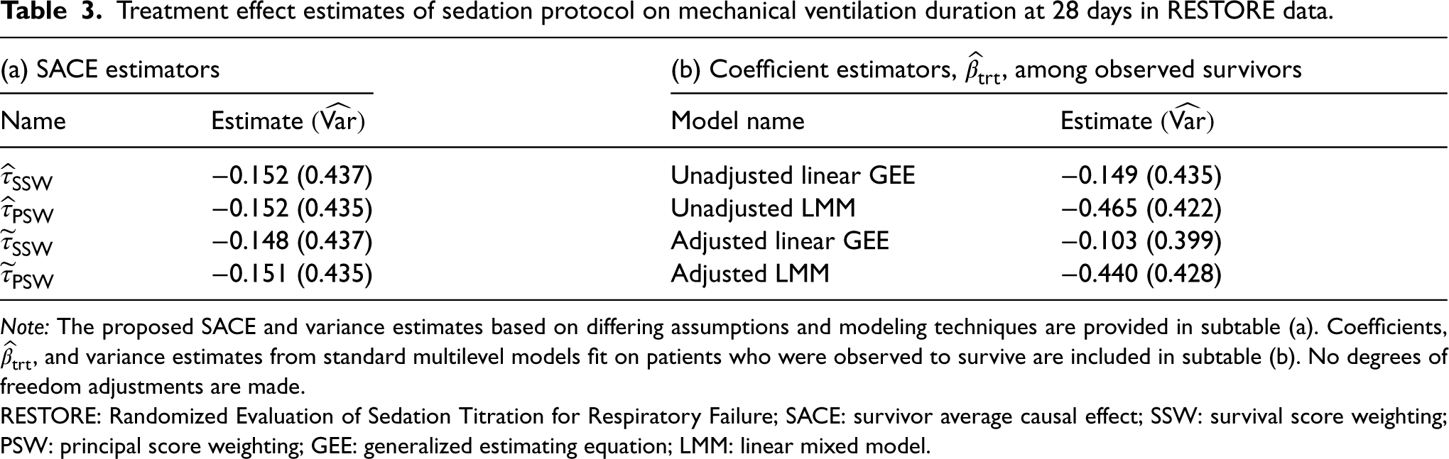
We apply our weighting estimators of SACE to the RESTORE data, where the survival status models adjust for variables suggested in the initial analysis. ⁴⁹ The covariates are age in years, Pediatric Risk of Mortality (PRISM) III-12 score (on log-scale), an aggregated measure of physiological status, ⁵² and Pediatric Overall Performance Category (POPC) > 1, an assessment of functional morbidity and cognitive impairment, ⁵³ and for the GLMM, there is a random intercept for PICU facility. The SACE estimates where survival status is modeled using a mixed effects logistic regression model are ${\hat{\tau }}_{\text{SSW}}=-0.152(-1.657,1.353)$ and ${\hat{\tau }}_{\text{PSW}}=-0.152(-1.652,1.349)$ . The SACE estimates where survival status is modeled using a logistic regression model are similar ${\tilde{\tau }}_{\text{SSW}}=-0.148(-1.621,1.325)$ and ${\tilde{\tau }}_{\text{PSW}}=-0.151(-1.621,1.319)$ . All standard errors are computed using the proposed sandwich variance estimators with a degrees of freedom correction. As displayed in Table 3, differences between the sandwich variance estimates (uncorrected) are negligible, which is expected because the estimated ICC for survival is small, only $0.026$ . The point estimates suggest that the protocolized sedation reduces duration on mechanical ventilation among always-survivors on average by $\sim$ 3.6 hours, but this effect is not statistically significant at the 0.05 level.

Table 3.

Treatment effect estimates of sedation protocol on mechanical ventilation duration at 28 days in RESTORE data.

(a) SACE estimators			(b) Coefficient estimators, ${\hat{\beta }}_{\text{trt}}$ , among observed survivors
Name	Estimate $(\widehat{\text{Var}})$		Model name	Estimate $(\widehat{\text{Var}})$
${\hat{\tau }}_{\text{SSW}}$	−0.152 (0.437)		Unadjusted linear GEE	−0.149 (0.435)
${\hat{\tau }}_{\text{PSW}}$	−0.152 (0.435)		Unadjusted LMM	−0.465 (0.422)
${\tilde{\tau }}_{\text{SSW}}$	−0.148 (0.437)		Adjusted linear GEE	−0.103 (0.399)
${\tilde{\tau }}_{\text{PSW}}$	−0.151 (0.435)		Adjusted LMM	−0.440 (0.428)

Note: The proposed SACE and variance estimates based on differing assumptions and modeling techniques are provided in subtable (a). Coefficients, ${\hat{\beta }}_{\text{trt}}$ , and variance estimates from standard multilevel models fit on patients who were observed to survive are included in subtable (b). No degrees of freedom adjustments are made.

RESTORE: Randomized Evaluation of Sedation Titration for Respiratory Failure; SACE: survivor average causal effect; SSW: survival score weighting; PSW: principal score weighting; GEE: generalized estimating equation; LMM: linear mixed model.

Due to conditional survival independence and survival monotonicity, the Set 1 and Set 2 identification assumptions are mutually exclusive, so from a causal perspective, it is instructive to consider which set is more suited to this data application (supposing correct representation of the randomization scheme). Given that sedation practices are not meant to directly treat the conditions associated with acute respiratory failure, the causal assertion that survival under the active treatment is no worse than under the control treatment may not be easily justified. On the other hand, the conditional independence assumptions for Set 1 may be plausible since the key covariates that potentially impact and differentiate patient survival events are identified in the original analysis plan. All that said, while the Set 2 assumptions seem reasonable for this particular CRT, they nor those for Set 1 are testable using the observed data alone, but the nearly identical results for SSW and PSW estimators lend empirical credence to their robustness relative to whichever underlying identification assumptions hold.

As a follow-up illustration, we fit unadjusted and adjusted standard multilevel models to the RESTORE data removing patients whose death was reported prior to 28 days. The models are a generalized estimating equation (GEE) with Gaussian-type mean and variance functions with an independence working correlation, also known as linear regression with cluster-robust standard errors, and a LMM with a random intercept for PICU. We consider these models as they are among the commonly used regression methods for analyzing CRTs but may not produce causal estimates in the presence of truncation by death. In Table 3, the non-mortal treatment effect estimate, which is the coefficient of treatment ${\hat{\beta }}_{\text{trt}}$ in the models, is reported alongside the variance estimate, $\widehat{\text{Var}}$ $({\hat{\beta }}_{\text{trt}})$ . These values are juxtaposed with the estimates for SACE. We observe that the results for the unadjusted GEE are similar to those that we have with the SACE estimators. However, ${\hat{\beta }}_{\text{trt}}$ does not target a clearly interpretable causal estimand because conditioning on survival breaks the balance of confounders across treatment groups and can lead to comparisons defined on different subpopulations. The similarity in estimates alone does not support the general application of such methods due to the ambiguity in the target estimand and may likely be attributed to the relatively low mortality rates in the RESTORE trial. Moreover, we see that the estimates for the remaining models, in particular the LMMs, are not comparable to those that we obtained for our SACE estimators. These differences may in fact be related to the selection bias introduced by conditioning on survivors and any distributional assumptions about the observed outcome. In contrast, the weighting methods avoid the need to consider outcome models that are often difficult to correctly specify, and they only require selecting a binary regression model to capture the likelihood of survival until the time of outcome measurement.

5. Discussion

For randomized trials targeting the effect of a binary treatment on a non-mortal outcome, participants who do not survive to their follow-up visit will have truncated outcome measurements. Estimating effects conditional on realizations of post-treatment variables such as survival status is a well-known potential source of selection bias that depends on underlying causal pathways. Moreover, when clusters are the randomization unit as in CRTs, there is an additional source of variation in patient outcomes due to within-group correlation. For this multifaceted problem, we target the SACE, a treatment effect conditional on individuals who would survive under either treatment received, and we discuss two sets of assumptions that allow for point identification of the SACE, notably accounting for unobservable sources of variation via a group-level latent variable. We develop two corresponding estimators for the SACE, denoted by SSW and PSW, based on the theory of M-estimation, where their asymptotic distributions have sandwich variance expressions enabling cluster-robust variance estimation.

Results of the simulation studies, which vary both the magnitudes of the within-cluster correlation and the treatment effect for survival status, suggest that the SACE estimators perform well in terms of empirical bias, and their confidence intervals generally achieve nominal coverage even for a small to modest number of clusters. There are occasional issues in undercoverage, but sources of this phenomenon have been documented in the past and may simply be remedied by other choices of small-sample corrections. Critically, both the SSW and PSW estimators prove to be robust to violations to one of their identifying assumptions—conditional survival independence for SSW and survival monotonicity for PSW. Furthermore, for these estimators, we consider models to predict survival status that do and do not explicitly address within-cluster correlation : mixed effects logistic regression (a type of GLMM) and logistic regression (a type of GLM), respectively. Performance in simulations across these modeling decisions is similar. Nevertheless, from the standpoint of addressing latent cluster-induced variation, the GLMM is a more principled approach compared to the GLM, and the simulation study shows that the empirical bias for the SACE estimator is in general smaller when the former is used. But, we demonstrate that in finite samples where the ICC for survival is also relatively low, the choice to use a GLMM may not be as stable (due in part to numerical methods), and one may prefer the GLM with a cluster-robust variance expression for inference, except if there is a previously known large effect of the treatment on survival. The above observations bear out in our application to the RESTORE data, where there are negligible differences in SACE interval estimates across the assumption sets and modeling choices. However, the SACE estimates may differ from estimation of treatment effects among observed survivors, which have no causal interpretation, and the magnitude of this difference may be amplified by (incorrect) assumptions when modeling the outcome distribution. To enable users to implement our methods, we provide an R package, PtSaceCrts, for computing SACE interval estimates based on choices of the set of assumptions and survival status model, available at https://github.com/abcdane1/PtSaceCrts. While we have a non-parametric bootstrap option in this package, the default estimation of asymptotic variances is computationally more efficient than bootstrapping and avoids complications of model fitting on bootstrapped samples when there is a small number of clusters.

The limitations and future considerations for our work relate to assumptions on and utilization of the data. For our analysis of the RESTORE study, we only consider the impact of the sedation protocol on mechanical ventilation duration over a fixed period of time, which does not make maximal use of the available data. Viewed as a time-to-extubation outcome, we could have performed a survival analysis examining treatment effect changes over time and accounting for censoring mechanisms. There has been recent literature on estimating SACE within the semi-competing risks framework for individually randomized data.^54–56 Aside from requiring causal censoring assumptions to be estimable, these estimands can be viewed as continuous time extensions of our target estimand but in the iid context. For identification of continuous time SACE estimands, all the existing approaches also include some framing of assumptions that allow teasing apart non-mortal and survival times across treatments, which enable specifying a likelihood from observable data and thus a range of estimation strategies. For example, Xu et al. ⁵⁶ employed a Set 1 like approach, replacing the conditional survival independence assumption with a slightly weaker Gaussian copula formulation with correlation parameter $\rho$ that allows defining the survival status models marginally and is identified for a fixed correlation (e.g. $\rho =0$ , as in our case). In this article, we do not pursue an extension of the aforementioned continuous time methods to estimate SACE in the CRT context which would require fully specifying a likelihood for estimation; instead we focus on simpler weighting estimators that are able to be applied to a variety of non-mortal outcomes (continuous, binary, and count). An extension of our methods to estimate continuous time SACE in CRTs with application to the RESTORE study is a direction for future research.

Additionally, the proposed estimation of the SACE estimand relies on cross-world identification assumptions, that is, worlds defined by intervening on $a=1$ and $a=0$ . This is a debated framework in causal inference because there is no setting, even hypothetically, where simultaneous interventions could occur and assumptions across them are able to be verified. ²¹ As an alternative framework, Stensrud et al. ⁵⁷ proposed estimands based on the notion of separable effects which avoid these cross-world assumptions and can be applied to the truncation by death problem. But, separable effects requires a significant conceptual exercise itself—one of decomposing treatment disjointly into its effect on survival and its effect on the non-mortal outcome. Despite the inherent untestability of cross-world assumptions, we opt for them because we feel that these assumptions as well as the SACE estimand that they identify are more easily translated to language accessible to practitioners. We have also assumed that there is no (marginal) dependence between the individual-level survival and non-mortal outcomes and cluster size (i.e. no informative cluster size), which can impact the validity of the proposed estimators for targeting individual-level effects. ²⁰ When informative cluster size is present, cluster-average and individual-average causal estimands may not overlap, necessitating a more principled approach to defining identification assumptions and compatible estimators as others have ventured at in recent literature in the absence of truncation by death. ⁵⁸ Another fundamental assumption is related to the mechanism of randomization, where we suppose that our data come from parallel-arm CRTs. However, a comprehensive review of analyses of CRTs in critical care units shows that less than half of them are based on true parallel-arm trials with the remaining being crossover or stepped wedge. ⁵⁹ The emergence of these types of randomized trials, motivated by practical, ethical, and statistical reasons, warrants an exploration of estimands for SACE that can accommodate different randomization designs.

Supplemental Material

sj-pdf-1-smm-10.1177_09622802241309348 - Supplemental material for Weighting methods for truncation by death in cluster-randomized trials

Supplemental material, sj-pdf-1-smm-10.1177_09622802241309348 for Weighting methods for truncation by death in cluster-randomized trials by Dane Isenberg, Michael O Harhay, Nandita Mitra and Fan Li in Statistical Methods in Medical Research