
Abstract
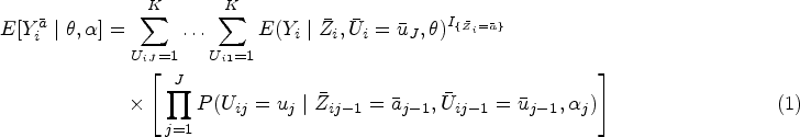
Bayesian methods are becoming increasingly in demand in clinical and public health comparative effectiveness research. Limited literature has explored parametric Bayesian causal approaches to handle time-dependent treatment and time-dependent covariates. In this article, building on to the work on Bayesian g-computation, we propose a fully Bayesian causal approach, implemented using latent confounder classes which represent the patient’s disease and health status. Our setting is suitable when the latent class represents a true disease state that the physician is able to infer without misclassification based on manifest variables. We consider a causal effect that is confounded by the visit-specific latent class in a longitudinal setting and formulate the joint likelihood of the treatment, outcome and latent class models conditionally on the class indicators. The proposed causal structure with latent classes features dimension reduction of time-dependent confounders. We examine the performance of the proposed method using simulation studies and compare the proposed method to other causal methods for longitudinal data with time-dependent treatment and time-dependent confounding. Our approach is illustrated through a study of the effectiveness of intravenous immunoglobulin in treating newly diagnosed juvenile dermatomyositis.
Introduction
Many studies aim to estimate treatment effectiveness using longitudinal observational data obtained from disease registries and administrative databases. Such a design reflects real-world clinical practice and simplifies the data collection process without the expense, intensive planning and complex infrastructure required by randomized controlled trials.1,2 Treatment assignment under this design typically follows a clinician-driven decision process, where the treating clinician determines the treatment option using available demographic and past and current medical records.
There is an increased demand for Bayesian causal methods in applied comparative effectiveness research of rare diseases.3–5 The Bayesian method provides a probability summary of the treatment effectiveness which can be communicated more easily with patients and their families and allows investigators to assess treatment effectiveness under various clinical expert beliefs.
In recent years, several Bayesian approaches, such as Bayesian propensity score analysis (BPSA), Bayesian marginal structural models (BMSMs) and Bayesian g-computation, and nonparametric/semiparametric Bayesian approaches for dynamic treatment regimes have been proposed to handle time-dependent treatment.6–13 In particular, BMSM and BPSA are not conventional full Bayesian approaches – the treatment assignment process under the ‘design’ stage is separated from the outcome process under the ‘analysis’ stage.7,9 These methods implement a ‘feedback-cutting’ strategy to ensure parameters from the treatment and outcome models are not estimated simultaneously. Both BPSA and BMSM employ Bayesian posterior predictive inference for estimating the inverse probability of treatment weighting (IPTW) weights (or importance sampling weights in the case of BMSM). Bayesian g-computation, 11 unlike standard g-computation, features joint modelling of the outcome, treatment and covariate processes where all processes are parametrically specified. This can be computationally intractable with a large set of time-dependent confounders without the use of shrinkage priors and other Bayesian variable selection methods. We direct readers to Li et al. 14 for a comprehensive review of Bayesian causal inference frameworks and methods.
Previously, methodology for handling latent confounders has been largely focused on methods to overcome violation of the no unmeasured confounding assumption.15–26 The use of latent variables in Bayesian causal modelling has been predominately explored under the context of Bayesian sensitivity analysis for unmeasured confounding in a point-treatment setting19,22,24,27; here latent variables quantify the impact of the unmeasured confounder on the treatment and outcome. The goal of the Bayesian sensitivity analysis is to estimate the bias-corrected causal effects. Additionally, causal modelling with latent class analysis has been explored to quantify the effect of an exposure effect on the latent outcome class membership.28,29 Our proposed Bayesian method differs from these works in three ways: first, we allow the latent confounder class to be visit-dependent; second, we use this visit-specific latent class as a means of modelling a large set of measured covariates in order to characterize time-dependent confounding. Lastly, we conduct our Bayesian inference using a joint likelihood for outcome, treatment and confounders.
The objective of this work is to propose a fully Bayesian causal model and estimation method that features dimension reduction of time-dependent confounders and at the same time enables the joint modelling of treatment, outcome and covariates. We propose a Bayesian latent class approach with a set of binary time-dependent covariates as class indicators (or manifestation variables) from a time-dependent latent confounder class. The proposed Bayesian latent class approach involves jointly modelling the treatment and outcome processes through the unobserved latent confounder classes and can be directly implemented in standard Markov chain Monte Carlo (MCMC) software (e.g. JAGS, Stan, etc).
In this article, we form our longitudinal causal structure with latent classes and formulate the proposed Bayesian approach in Section 2. Simulation studies are conducted in Section 3 to assess the estimation performance with varying sample sizes, numbers of indicators, the quality of indicators, as well as misspecified outcome and/or treatment assignment model. The motivating study is analysed in Section 4 and we conclude with a discussion in Section 5.
Bayesian estimation in a longitudinal causal framework via latent classes
Notation
Let
Causal diagram with latent classes
In this article, we consider a new causal structure with time-dependent latent classes as displayed in Figure 1. We assume at each visit
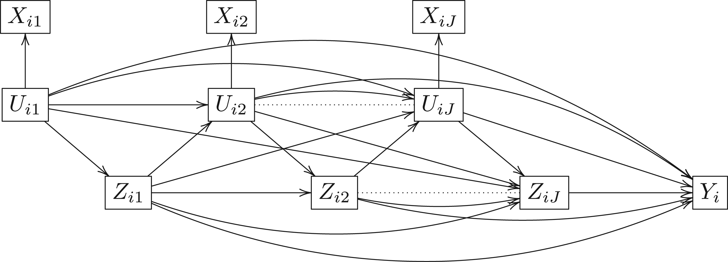
Longitudinal causal directed acyclic graph.
Under this causal framework, the set of time-varying indicators do not directly affect treatment assignment (i.e. the indicators are conditionally independent of treatment given latent class) or the end-of-study outcome
Following Rubin’s potential outcome framework, for each unique treatment sequence
Stable unit treatment value assumption. We assume no competing of treatment resources between patients, that is, that the treatment assignment for one patient does not affect the outcome of another and Sequential latent unconfoundedness. Treatment assignment at each visit is independent of potential variables, given the history of treatment and latent class, such that, Conditional independence between class indicators. We assume conditioning on the latent class
The causal parameter of interest is the average potential outcome
The challenge here is that
Let
We estimate the average potential outcome using posterior predictive inference where we predict the end-of-study outcome of a targeted, static treatment sequence Given With
Under the full Bayesian estimation following the joint likelihood in (2), the unobserved latent classes are imputed (or in other words predicted) at each Monte Carlo iteration along with posterior draws of all model parameters. However, the imputed latent classes are not directly used to estimate the average potential outcome, instead, the posterior probability of being in a specific class conditioning on past latent classes, past treatment and class indicators is used.

For this work, we assume the number of latent classes at each visit is finite, fixed and known. This means the treating clinician classifies patients into a fixed number of latent classes at each visit and such information is available to the analyst. Standard statistical information criteria including the Bayesian information criterion and the deviance information criterion (DIC) can be used in practice to select the number of latent classes and determine the fit of the Bayesian latent class approach.34,35
Simulation with latent confounder class
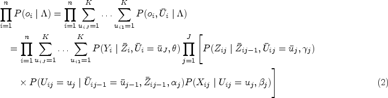
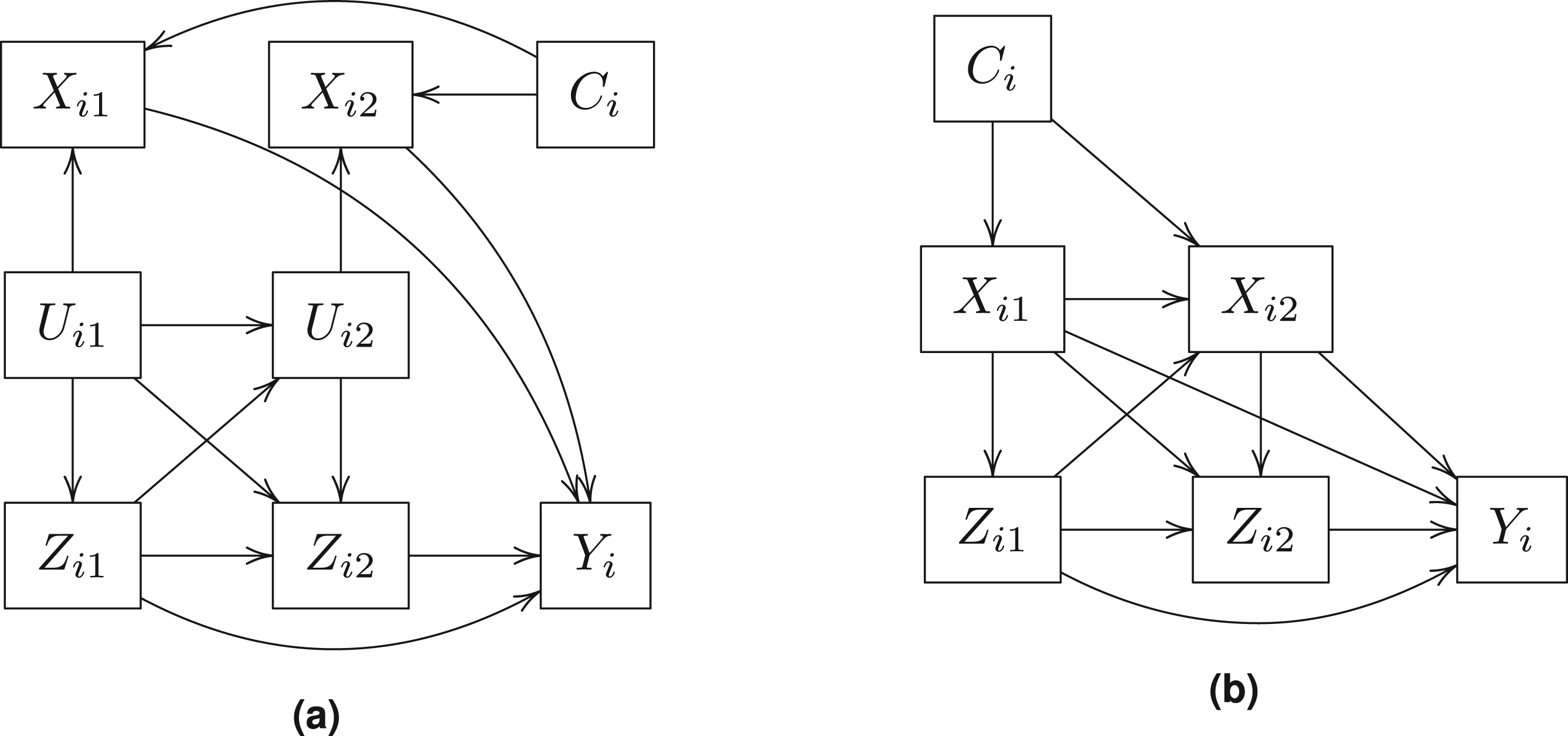
We consider a simulation study with 1000 replications of a simple three-visit longitudinal study of 125, 250, and 500 subjects. Figure 2 displays the causal diagram of the simulated data. The simulated data consists of a continuous and a binary time-independent confounder
Longitudinal causal diagram of the simulation dataset with latent confounder class.
The simulated datasets are generated as follows:
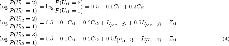
We generate The class indicators are Bernoulli random variables that are conditionally independent given High-quality indicators: Medium-quality indicators: Low-quality indicators: The end-of-study continuous outcome We define medium level latent class confounding as We define high level latent class confounding as Adjusted linear regression on the outcome,
Standard marginal structural model (MSM) without latent classes (treating class indicators as time-dependent confounders) uses the visit-specific treatment assignment model to obtain visit-specific IPTW weights, specifically
Longitudinal targeted maximum likelihood estimation (TMLE) without latent classes where we fit the treatment assignment model in (8) and the outcome model in (7).36–38
For this simulation study, the causal parameter of interest is the causal contrast in the outcome between ‘always treated’ and ‘never treated’,
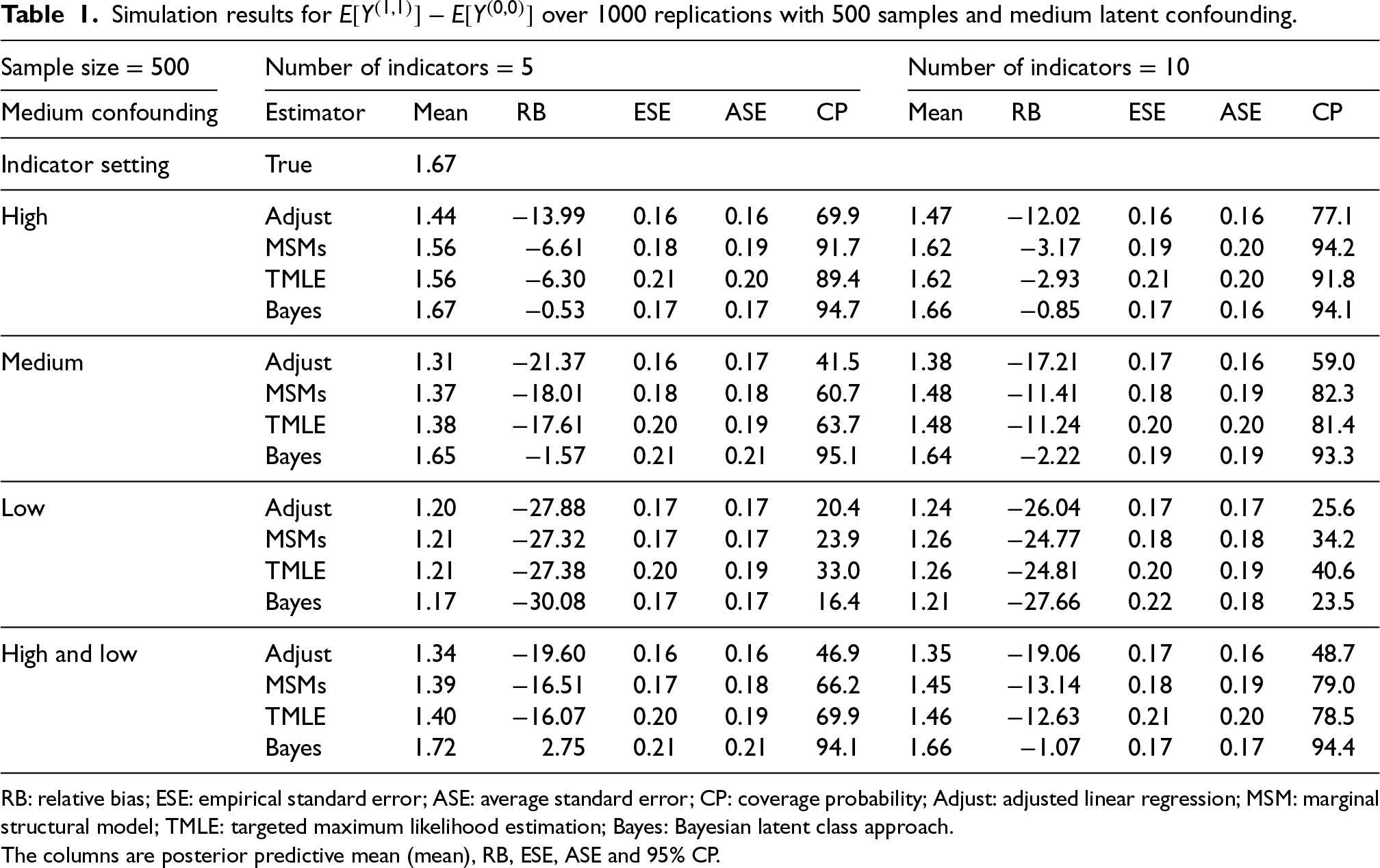
We consider four indicator quality combinations: all indicators are of high quality, all indicators are of medium quality, all indicators are of low quality and a mixed setting where one indicator for latent class 1 was high quality and the others were low quality (i.e.
We use diffuse normal priors,


From Table 1, the Bayesian latent class approach outperforms others in the presence of medium- to high-quality class indicators. Specifically, the Bayesian latent class approach produces the least biased estimates when all indicators are of medium or high quality and when there is one high-quality indicator and all the others are low quality. However, when all indicators are of low quality, all methods return biased estimators and the Bayesian latent class approach produces the most biased estimates. Comparing the frequentist methods, the conventional MSM and TMLE without latent classes perform equally well with medium- to high-quality indicators. With a sample size of 500 and a medium level of latent confounding, as the number of indicators increased from 5 to 10, the estimation of the causal contrast
Simulation results for
RB: relative bias; ESE: empirical standard error; ASE: average standard error; CP: coverage probability; Adjust: adjusted linear regression; MSM: marginal structural model; TMLE: targeted maximum likelihood estimation; Bayes: Bayesian latent class approach.
The columns are posterior predictive mean (mean), RB, ESE, ASE and 95% CP.
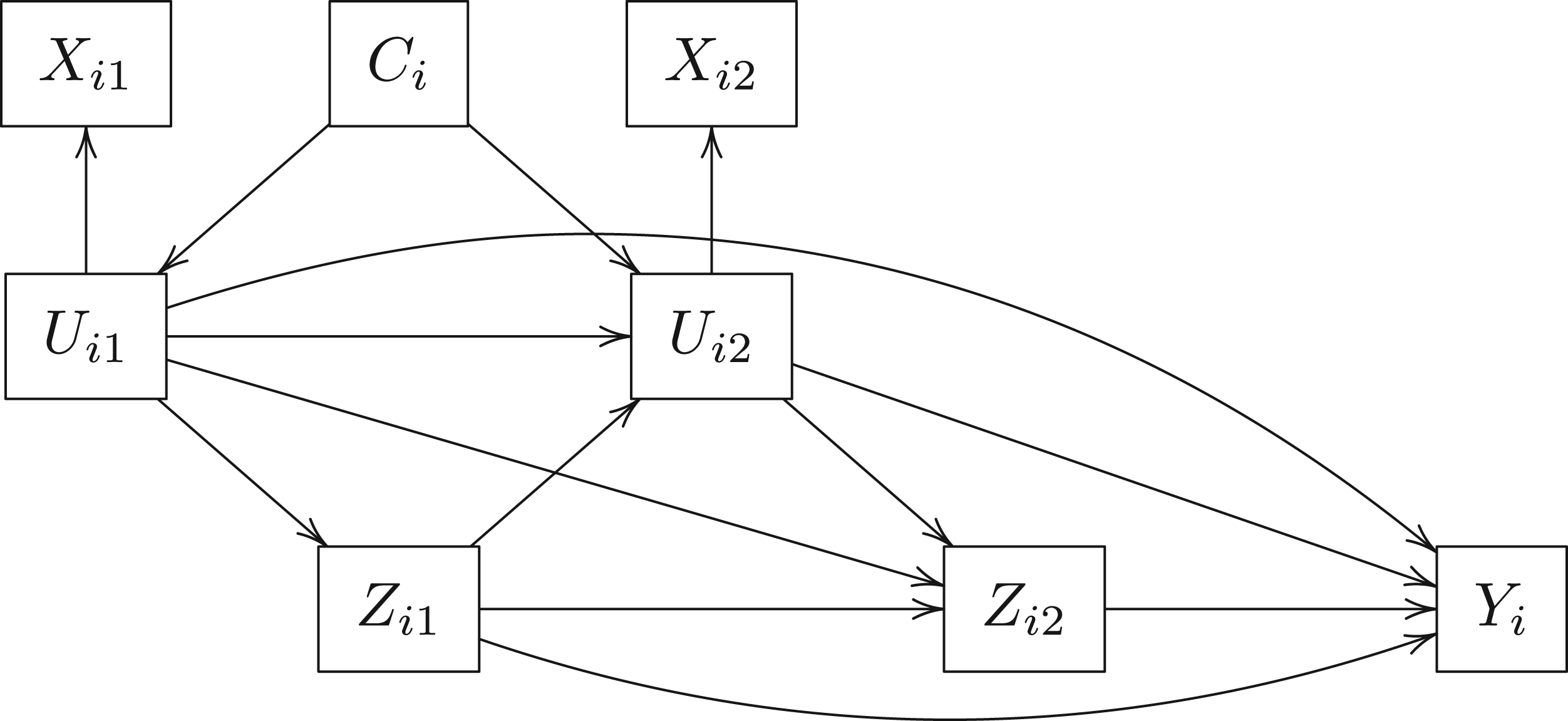
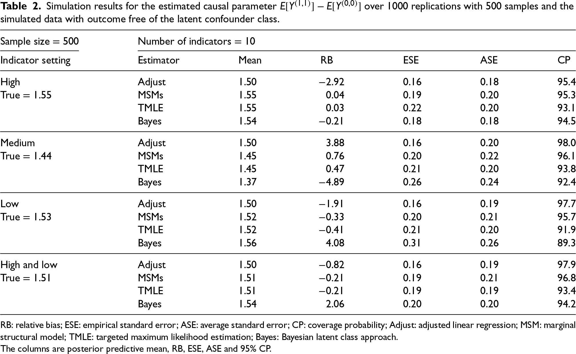
To explore the performance of the Bayesian method under misspecification, we consider another two simulation studies with 1000 replications of a simple three-visit longitudinal study of 500 subjects where (i) the outcome variable is not directly affected by the latent confounder classes, and (ii) the latent confounder class is not featured in the causal framework. Figure 3(a) displays the causal diagram of the simulated data where the outcome model is free of the latent confounder class and Figure 3(b) displays the causal diagram of the simulated data where the treatment and outcome models are free of the latent confounder class. Simulation details are described in the online Supplemental material.
Longitudinal causal diagram of the simulation dataset without latent confounder.
The simulation results with a misspecified outcome model are reported in Table 2 (
Simulation results for the estimated causal parameter
RB: relative bias; ESE: empirical standard error; ASE: average standard error; CP: coverage probability; Adjust: adjusted linear regression; MSM: marginal structural model; TMLE: targeted maximum likelihood estimation; Bayes: Bayesian latent class approach.
The columns are posterior predictive mean, RB, ESE, ASE and 95% CP.
Simulation results for the estimated causal parameter
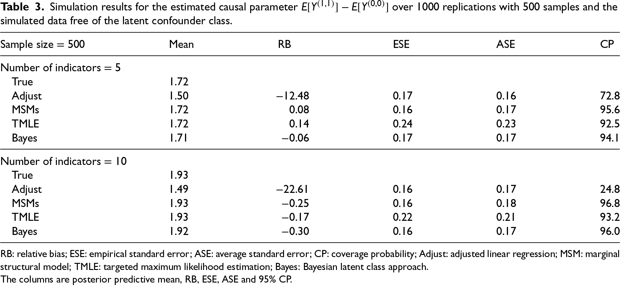
RB: relative bias; ESE: empirical standard error; ASE: average standard error; CP: coverage probability; Adjust: adjusted linear regression; MSM: marginal structural model; TMLE: targeted maximum likelihood estimation; Bayes: Bayesian latent class approach.
The columns are posterior predictive mean, RB, ESE, ASE and 95% CP.
Overall, the performance of the Bayesian method was unchanged when the outcome is directly influenced by the indicators rather than the latent classes (under misspecified outcome model) (Table 2). Although slightly more biased than the frequentist methods, the Bayesian approach has little bias when all indicators are of medium or high quality and the bias difference reduces as the number of indicators increases. Having at least one high-quality indicator results in approximately unbiased estimators for all methods. However, when all indicators are of poor quality, the Bayesian method is biased while the frequentist methods return approximately unbiased estimators (Table 2). Lastly, the Bayesian latent class approach continues to do well when data are simulated without latent classes (Table 3).
We applied the proposed Bayesian latent class approach to a retrospective cohort study of intravenous immunoglobulin (IVIg) in treating JDM using observational clinical data hosted at The Hospital for Sick Children (SickKids). JDM is a rare, chronic multisystem disease in children with incidence estimates of about 2–4 per million paediatric population in North America. 40 JDM is considered incurable at the moment and current treatment goals for managing newly diagnosed moderate JDM are to achieve inactive disease and prevent functional limitations. 5 An earlier version of the observational SickKids JDM data was analysed using marginal structural models, BPSMs and two-step BPSA to investigate the effect of IVIg adjunct therapy on successfully managing JDM disease activity, compared to the standard therapy without IVIg.12,41
The SickKids JDM data were recorded whenever a patient completed a scheduled clinical visit. The baseline visit
We defined the primary clinical outcome as the probability of achieving a score of zero on the Child Health Assessment Questionnaire (CHAQ) at 18 months. The CHAQ score, ranging between 0 and 3, is a functional assessment tool that measures the level of physical disability of children and its use has been validated in JDM. 42 A score of zero indicates that the patient can perform activities of daily living without any difficulty and a score of three indicates the patient can no longer complete activities of daily living. At baseline and each follow-up visit, patients were prescribed either the standard JDM therapy or IVIg in addition to the standard JDM therapy by the treating rheumatologist. Patients were defined as being exposed to IVIg at each clinical visit if during the six months prior a prescription of IVIg was recorded. In total, 34 out of the 121 patients (28.1%) were exposed to IVIg within the first 18 months post-diagnosis. We assumed clinicians at the baseline and follow-up visits used the following five clinical indicators to assign treatment: present functional status (normal vs. abnormal), currently taking prednisone (yes vs. no), presence of Gottron’s papules, presence of heliotrope rash, and presence of abnormal nailfold capillaries.
Patients who were exposed to IVIg typically remained on IVIg for a few follow-up visits.
41
Therefore, we are interested in the causal contrast in the probability of achieving daily living without any level of difficulty at 18 months between patients who were exposed to IVIg and remained on IVIg up to 18 months (‘always treated’) and patients who were IVIg free for 18 months (‘never treated’). In addition to the Bayesian latent class approach, all four frequentist methods included in the simulation study were applied to the JDM data. We fitted two Bayesian latent class models, one with two latent confounder classes at each visit and one with three latent confounder classes at each visit. The final Bayesian model was selected using the DIC (the smallest of the two models). We used diffuse normal priors (i.e.
The baseline CHAQ score was higher for patients who were exposed to IVIg compared to patients who were IVIg free within the first 18 months with the median CHAQ score valued at 1.63 for IVIg-exposed patients and the median CHAQ score valued at 1.06 for IVIg free patients. Over the study period, we observed an overall decrease in the CHAQ score for all patients (Figure 4). The majority of patients who started on IVIg remained on IVIg in subsequent visits. In total, 13 out of the 34 IVIg-exposed patients (38%) received IVIg since baseline and remained on IVIg for up to 18 months.
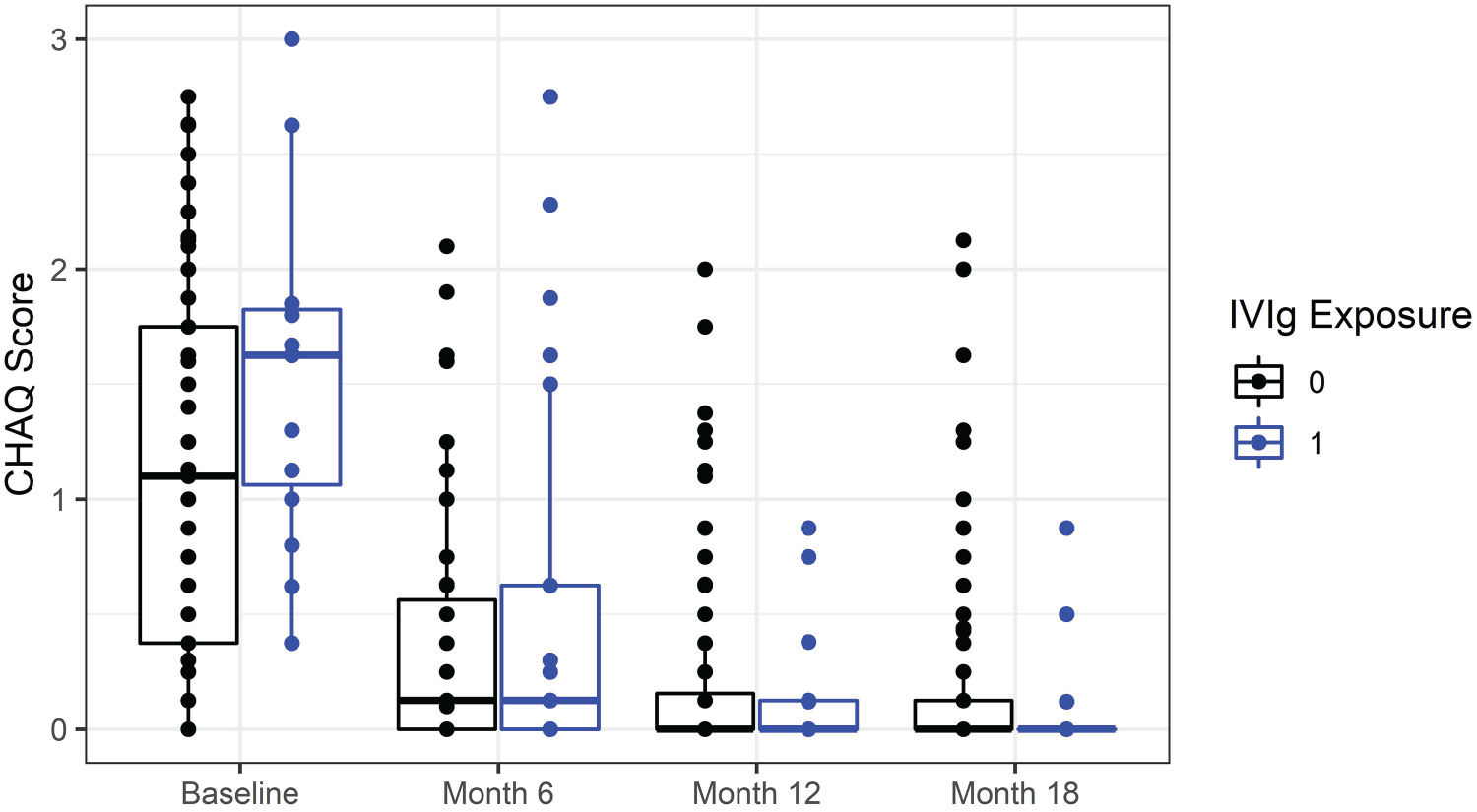
CHAQ score distribution overtime by IVIg exposure within 18 months since diagnosis. CHAQ: child health assessment questionnaire; IVIg: intravenous immunoglobulin.
The DIC for the Bayesian model assuming two latent classes at each visit was 2905.2, while the DIC for the Bayesian model assuming three latent classes at each visit was 2924.9. Therefore, the Bayesian latent approach with two latent classes was selected. A trace plot of the causal parameter of interest is included in the Supplemental material (Figure S2). Table 4 examines the estimation stability of the latent class model, by showing the number and proportion of JDM patients who had their visit-specific latent class being consistently predicted across MCMC iterations. Consistently predicted latent classes were determined using the subject-visit specific posterior probability of being in each of the two classes with at least 90% or 80% probability. At baseline, it was possible to determine 75% of patients’ latent classes with at least 90% certainty and to determine 93% of patients with at least 80% certainty. Although the predicted probability of being in each class was reduced over follow-up visits, the majority of patients had their time-dependent latent classes identified with at least 79% certainty at follow-up visits.
Number of juvenile dermatomyositis subjects across the total 18,000 Markov chain Monte Carlo iterations with consistently predicted latent class memberships.
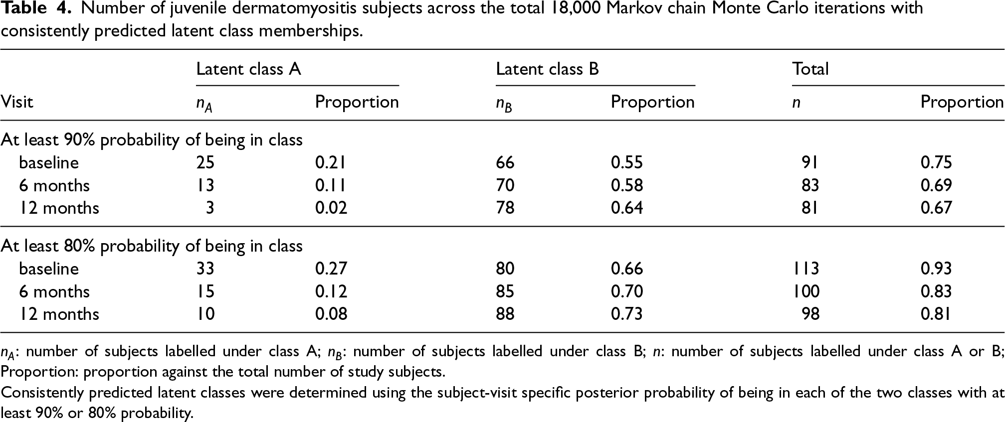
Consistently predicted latent classes were determined using the subject-visit specific posterior probability of being in each of the two classes with at least 90% or 80% probability.
The estimated causal contrast of interest – the probability difference of achieving no living difficulty at 18 months between always treated and never treated, is presented in Table 5. G-computation, TMLE and the mode of the posterior predictive distribution under the Bayesian latent class approach were similar. Since only 34 patients were exposed to IVIg, MSMs might be sensitive to the time-dependent treatment assignment model specification. As expected, the TMLE estimate had the largest standard error compared to other methods. Although the point estimates of the causal contrast were all positive, all of the 95% confidence intervals corresponding to the four frequentist methods included zero, indicating a statistically insignificant difference in the outcome.
The estimated absolute risk difference on achieving no living difficulty at 18 months between always treated and never treated.
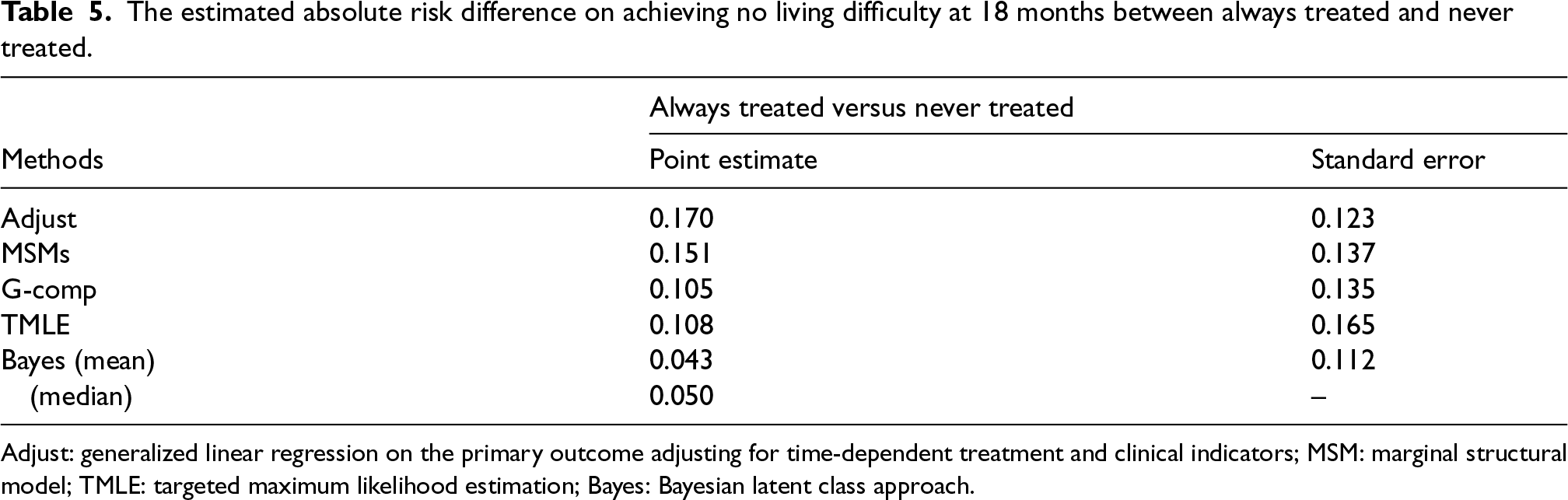
Adjust: generalized linear regression on the primary outcome adjusting for time-dependent treatment and clinical indicators; MSM: marginal structural model; TMLE: targeted maximum likelihood estimation; Bayes: Bayesian latent class approach.
In addition to point estimates, the Bayesian method gives a probability distribution for the risk difference (Figure 5). Under the Bayesian latent class approach, we can conclude that there is a 69% chance of observing a higher probability of achieving no living difficulty (a risk difference >0) at 18 months under always treated compared to never treated. We can also easily assess the likelihood of observing other clinically relevant risk differences.
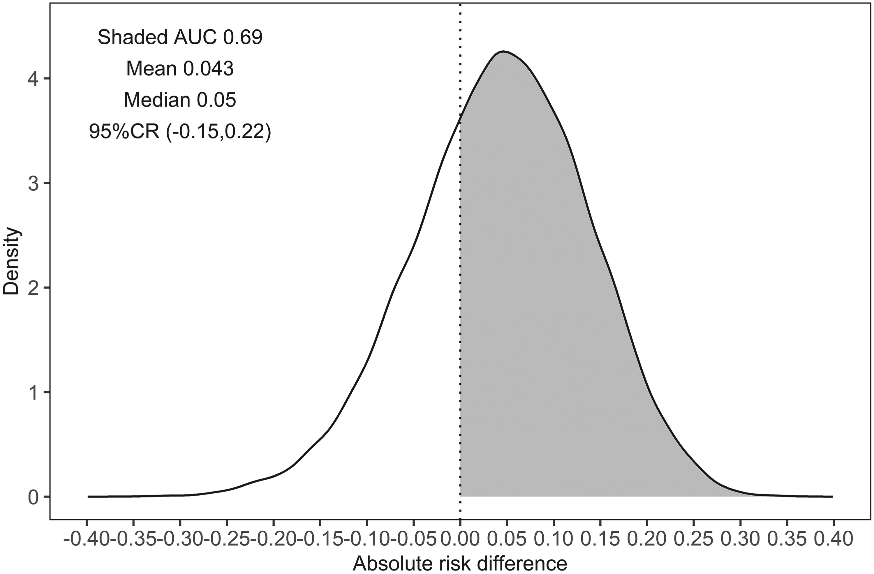
Posterior predictive distribution of the estimated probability difference on achieving no living difficulty at 18 months between always treated and never treated. AUC: area under the curve; CR: credible region.
In this article, we presented and demonstrated a Bayesian latent class approach to conduct causal inference with time-dependent treatment and time-dependent confounding. The introduction of the visit-specific latent confounder class to the causal framework permits a full Bayesian estimation of the causal effects via posterior predictive inference and naturally achieves dimension reduction of the confounders. Based on the simulation study, the proposed Bayesian latent class approach performs well when the clinician-driven treatment assignment follows the hypothesized unobserved classification process with medium- to high-quality class indicators. Furthermore, the Bayesian latent approach still achieves approximately unbiased estimation when the true outcome process is free of the latent confounder class as well as when both the true outcome and treatment assignment processes are free of the latent confounder class.
The proposed Bayesian latent class approach has a few advantages over existing Bayesian causal inference methods, namely, the parametric Bayesian g-computation and Bayesian MSMs. Compared to Bayesian g-computation, the Bayesian latent class approach is simpler to specify the joint distribution of a potentially large number of confounding indicators. 11 Additionally, compared to Bayesian MSMs, the Bayesian latent class approach is fully Bayesian.9,12 Our approach has the potential to overcome unmeasured confounding (in the form of unmeasured class indicators), if the observed class indicators are sufficient to infer the distribution of the latent confounder class and the treatment assignment mechanism follows the clinician-driven classification process.
In this work, we have assumed that there is a true underlying latent class
The estimation unbiasedness of the Bayesian latent class approach depends on the quality of the class indicators and the number of class indicators (although less sensitive to the latter). A post-hoc approach to examine indicator quality, as used in the applied JDM analysis, is by investigating the posterior predicted latent class membership. If most patients under the Bayesian latent class model have at least 90% of the predicted latent class membership being identical across posterior draws, we can argue the latent class model is fitted with good quality indicators.
In some cases, it is easy to verify the clinician-driven treatment assignment follows a classification process (e.g. studies that conducted at a single clinical centre with a small number of treating physicians), but in others less so (e.g. multicenter or multinational studies). It is reassuring that the Bayesian latent class approach achieved unbiased estimation in the two simulation studies with misspecified models. In the applied JDM analysis, without the knowledge of the treatment assignment mechanism, the Bayesian latent class approach returned similar point estimates and standard error compared to popular frequentist causal methods. In application, we recommend the use of standard information criteria such as DIC to assess the fit of the Bayesian latent class model, in particular, when comparing different latent class models with varying numbers of latent classes.
The proposed latent class causal mechanism in this article assumes no direct causal pathways connecting the time-dependent class indicators to the treatment and the outcome and that only time-independent confounders (acting as latent class model covariates) are considered as presented in the simulation study. A few alternative and more generalized causal mechanisms with latent confounder classes would be of interest in future work including causal structures with arrows pointing from the class indicators to the treatment, the outcome and time-dependent covariates with arrows pointing to the latent classes. The proposed latent class approach requires a binary class indicator. In future work, the latent class model can be extended with a mixture of continuous and dichotomized class indicators and a time-dependent number of latent classes.
In summary, our proposed Bayesian latent class approach performed well with medium- to high-quality indicators, was robust to the studied forms of misspecification, and remains tractable in the presence of high-dimensional confounders. We thus suggest that analysts consider it in cases where it is plausible that a latent disease classification drives both disease outcomes and treatment decisions.
Supplemental Material
sj-pdf-1-smm-10.1177_09622802241298704 - Supplemental material for A Bayesian latent class approach to causal inference with longitudinal data
Supplemental material, sj-pdf-1-smm-10.1177_09622802241298704 for A Bayesian latent class approach to causal inference with longitudinal data by Kuan Liu, Olli Saarela, George Tomlinson, Brian M Feldman and Eleanor Pullenayegum in Statistical Methods in Medical Research
Footnotes
Acknowledgements
The authors thank Ingrid Goh for facilitating access to the Hospital for Sick Children JDM clinical data.
Declaration of conflicting interests
The authors declared no potential conflicts of interest with respect to the research, authorship, and/or publication of this article.
Funding
The authors disclosed receipt of the following financial support for the research, authorship, and/or publication of this article: This research was supported by funding from a Canadian Institutes of Health Research Doctoral Award (Frederick Banting and Charles Best Canada Graduate Scholarship) and the Connaught New Researcher Award to the first author.
Supplemental material
Supplemental material for this article is available online.
References
Supplementary Material
Please find the following supplemental material available below.
For Open Access articles published under a Creative Commons License, all supplemental material carries the same license as the article it is associated with.
For non-Open Access articles published, all supplemental material carries a non-exclusive license, and permission requests for re-use of supplemental material or any part of supplemental material shall be sent directly to the copyright owner as specified in the copyright notice associated with the article.