
Abstract
The use of genetic variants as instrumental variables – an approach known as Mendelian randomization – is a popular epidemiological method for estimating the causal effect of an exposure (phenotype, biomarker, risk factor) on a disease or health-related outcome from observational data. Instrumental variables must satisfy strong, often untestable assumptions, which means that finding good genetic instruments among a large list of potential candidates is challenging. This difficulty is compounded by the fact that many genetic variants influence more than one phenotype through different causal pathways, a phenomenon called horizontal pleiotropy. This leads to errors not only in estimating the magnitude of the causal effect but also in inferring the direction of the putative causal link. In this paper, we propose a Bayesian approach called
Keywords
1 Introduction
Finding and estimating causal effects from various measured exposures (phenotypes, biomarkers, risk factors) to disease and health-related outcomes is a crucial task in epidemiology. If we knew there was a causal link from a modifiable exposure (e.g. the level of low-density lipoprotein cholesterol (LDL-C)) to an outcome of interest (e.g. the incidence of cardiovascular disease), we could intervene on the former to produce a desired effect on the latter. Moreover, if we knew the magnitude of the causal effect, we could then predict the efficacy of treating the disease by altering the level of the exposure.
Randomized controlled trials (RCTs) are the best means of establishing the causal relation between exposure and outcome. 1 In epidemiological research, RCTs have been used, for example, to identify causal risk factors or to determine the efficacy of a new drug. However, it is often not practical or ethical to perform an RCT, in which case we want to be able to extract causal information from observational epidemiological studies. Directly inferring causation from observational data is problematic since observed correlations (associations) do not imply any particular causal relationship on their own. The correlation between two variables X and Y can be explained by the existence of a causal link from X and Y (direct causation) or from Y to X (reverse causation), but it can also be explained by an unobserved common cause (confounder) influencing the two variables simultaneously. It can even be the result of a combination of causal and confounding effects.
One method for finding and estimating the magnitude of causal effects from observational data that has recently gained traction in the field of epidemiology is Mendelian randomization (MR). In MR, germline genetic variants are used as proxy variables for environmentally modifiable exposures with the goal of making causal inferences about the outcomes of the modifiable exposure. 2 The basic principle behind MR is that the differences between individuals resulting from genetic variation are not subject to the confounding or reverse causation biases that distort observational findings. 3 The natural “randomization” of alleles (variant forms) can thus be likened to the random allocation of treatment performed in RCTs in the sense that groups defined by the value of a relevant genetic variant will experience an on-average difference in exposure, while not differing with respect to confounding factors. 4
MR has already proved very useful in extracting causal information from observational studies. MR has been used successfully for drug target validation, for predicting side effects of drug targets, for discovering causal risk factors in clinical practice, or for a better understanding of complex molecular traits.
5
In a classic MR study, Chen et al.
6
examined the nature of the association between alcohol intake and blood pressure. In this example, the exposure variable (alcohol intake) is a modifiable behavior, but conducting an RCT would be problematic for both ethical and practical reasons: alcohol consumption is potentially damaging to the subject’s health and measuring the intake is prone to error. Chen et al.
6
employed the genetic variant ALDH2 as a surrogate for measuring alcohol intake (see Figure 1). ALDH2 encodes aldehyde dehydrogenase, a major enzyme involved in alcohol metabolism. The (*2*2) variant of the ALDH2 gene is associated with an accumulation of acetaldehyde in the body after drinking alcohol, and therefore unpleasant symptoms. Because of this, carriers of this particular variant tend to limit their alcohol consumption. Chen et al.
6
found that the individuals possessing the (*2*2) variant also have lower blood pressure on average. The authors considered the possibility that the (*2*2) genotype influences blood pressure via a different causal pathway not mediated by alcohol intake (horizontal pleiotropy). However, they found no association between ALDH2 and hypertension in females, for whom drinking levels in any genotype group were similar (very low). If there were pleiotropic effects, an effect on blood pressure would be seen in both sexes. The findings of Chen et al.
6
support the idea that alcohol intake increases blood pressure and the risk of hypertension, to a much greater extent than previously thought. Their results indicate that previous observational epidemiological studies suggesting the cardioprotective effects of moderate alcohol consumption might have been misleading.
Chen et al.
6
used the ALDH2 genetic variant as a proxy for alcohol intake to determine if there is a causal link between the latter and blood pressure. They found that alcohol intake has a marked positive causal effect on blood pressure.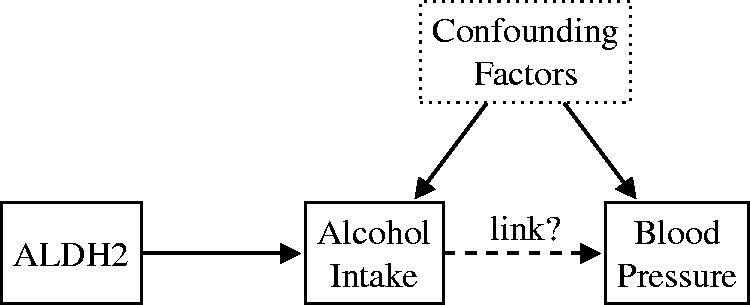
In a more recent study, Ference et al.
7
performed an MR meta-analysis for the purpose of estimating the effect of long-term exposure to lower-plasma LDL-C on the risk of coronary heart disease (CHD). Unlike in the previous example, the causal link from LDL-C to CHD was already well established at the time of the study, but the magnitude of the (long-term) causal effect had not been reliably quantified (see Figure 2). To estimate the causal effect of LDL-C exposure on the risk of CHD, Ference et al.
7
considered nine polymorphisms (genetic variations resulting in the occurrence of several different alleles at a locus) in six different genes. For each polymorphism, they computed a causal effect estimate using MR and then they combined the results to obtain a more precise estimate. Finally, they compared the estimated causal effect of long-term exposure to lower LDL-C with the clinical benefit resulting from the same magnitude of LDL-C reduction during treatment with a statin. Ference et al.
7
found that Mendelian random allocation to lower LDL-C levels was responsible for a 54.5% reduction in CHD risk for each mmol/L lower LDL-C. They concluded that prolonged (lifetime) exposure to lower LDL-C results in a threefold greater reduction in the risk of CHD compared to the clinical benefit of a statin-based treatment producing the same magnitude of LDL-C reduction.
Ference et al.
7
used Mendelian randomization for estimating the (positive) causal effect of low-density lipoprotein cholesterol (LDL-C) on the risk of coronary heart disease (CHD). They estimated that for each mmol/L lower LDL-C, the risk of CHD is reduced by 54.5% (95% CI (48.8%, 59.5%)).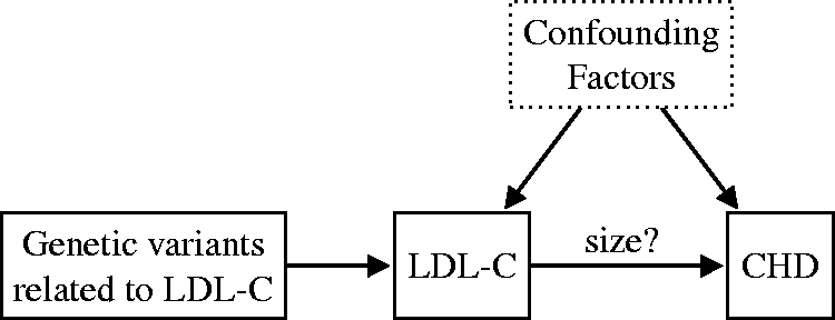
Finally, Vimaleswaran et al.
8
investigated the causality and direction of the association between body mass index (BMI) and 25-hydroxivitamin D (25(OH)D). In this example, it is not clear whether the larger vitamin D storage capacity of obese individuals (vitamin D is stored in fatty tissues) lowers their 25(OH)D levels or whether 25(OH)D levels influence fat accumulation. The latter is an example of reverse causation, which occurs when the outcome of interest precedes and leads to changes in the exposure instead of the other way around.
9
Reverse causation is an important source of bias in observational epidemiological studies,2,10 which can lead to misinterpretation in the observed association with respect to the potential impact of interventions.
11
In their work, Vimaleswaran et al.
8
used a bidirectional MR approach (see Figure 3), which implies performing an MR analysis in both directions, to distinguish between the two causal models. For this approach to work, it must be known on which phenotypic trait each genetic variant has a primary influence.
4
If vitamin D deficiency influences obesity, then the genetic variants primarily associated with lower 25(OH)D levels should also be associated with higher BMI. Conversely, if obesity leads to lower vitamin D levels, then the genetic variants primarily associated with higher BMI should also be related to lower 25(OH)D concentrations. Vimaleswaran et al.
8
concluded that higher BMI (obesity) leads to lower vitamin D levels and not the other way around. Their findings provided evidence for the role of obesity as a causal risk factor for vitamin D deficiency and suggested that interventions meant to reduce BMI are expected to decrease the prevalence of vitamin D deficiency, as later shown in intervention studies.12,13
Vimaleswaran et al.
8
explored the causal direction of the relationship between body mass index (BMI) and 25-hydroxivitamin D [25(OH)D] via bidirectional Mendelian randomization. They concluded that higher BMI leads to lower vitamin D levels and not the other way around.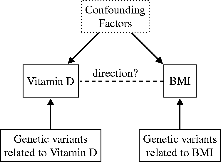
In this paper, we introduce a Bayesian framework (Bayesian approach to Mendelian randomization (
2 Instrumental variables and MR
2.1 Instrumental variable assumptions
MR is an approach in which genetic variants are used as instrumental variables for estimating the efffect of a modifiable phenotype or exposure on an outcome variable of clinical interest. A (valid) instrumental variable (IV) or instrument
14
is a factor which:
(IV1) is associated with the exposure; (IV2) is independent of all confounders of the exposure–outcome association; (IV3) influences the outcome only through its effect on the exposure.
The three core IV assumptions are depicted by the directed acyclic graph in Figure 4, where G is the genetic variant used as an instrumental variable, X is the variable measuring the exposure, Y is the variable measuring the outcome of interest, and U is an unmeasured variable that encapsulates the potential confounding effects affecting the exposure–outcome association. Note that for the graphical model to be acyclic, there must be no feedback loops in the system. Acyclicity is a standard assumption in MR and implies that the causal link of interest is unidirectional.
15
Assumption IV1 is represented in Figure 4 by the edge between G and X. Note that the association between the genetic variant and the exposure need not be causal, although this is often assumed in the context of MR. Assumption IV2 is denoted by a lack of paths from G to U. Finally, assumption IV3 is denoted by an absence of paths from G to Y, except for the one that goes through X. Genetic variants are particularly suitable as candidate instrumental variables because they are fixed at conception and “randomized” in a population according to Mendel’s laws of inheritance, meaning that their associations with non-genetic measures are generally not susceptible to confounding or reverse causation.5,10 In graphical terms, this is equivalent to removing all arrows from non-genetic variables (X,Y,U in Figure 4) to genetic variables (G in Figure 4).
Directed acyclic graph showing the instrumental variable assumptions. Causal effects are unidirectional and denoted by arrows. The association entailed by IV1 is highlighted in red, while the crossed-out dashed lines signify the absence of an association (causal or non-causal). The dotted border of U means that the variable is unobserved.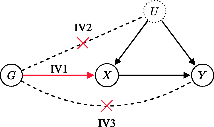
2.2 The MR pipeline
The suitability of using genetic variants as instrumental variables combined with the wide availability of data on genetic associations extracted by means of high-throughput genomic technologies have contributed to the increasing popularity of MR applications.4,16 The first step in MR is to find genetic variants that are robustly associated with the exposure under study. 17 Ideally, MR is performed using a single variant whose biological effect on the exposure is well understood. In practice, however, such a single variant is not always available or known. Moreover, genetic variants typically only explain a small proportion of the variance in the exposure. 18 When a single reliable genetic instrument is not available, it has become common to use multiple genetic variants in MR studies. Genome-wide association studies (GWAS) provide a rich source of potential instruments for MR analysis. 19 Increasing the number of exposure-related genetic variants will increase the proportion of variance explained by the instruments, which will lead to improved precision in the causal estimate and to increased power in testing causal hypotheses. 17 What’s more, the use of multiple genetic instruments provides opportunities to test for violations of the IV assumptions. 20
Genetic variants are typically selected based on the size of the genetic effect on the exposure of interest and the specificity of the association.
19
After deciding on a set of relevant exposure-related genetic instruments, the next step is to examine if they are also associated with the disease outcome. If no genotype-outcome association is found, then it becomes likely that there is no causal link from exposure to outcome. Otherwise, by making additional assumptions, it is possible to compute a consistent estimate of the causal relationship’s strength.
15
A commonly made assumption is that the causal relation between the exposure X and the outcome Y is linear


Unfortunately, when selecting multiple genetic variants for MR based on their association with the exposure, we cannot be certain that all of them are valid instrumental variables. In the worst possible case, none of the selected variants are valid instruments for the exposure–outcome associations. As a result, there is great interest in developing methods robust to the validity of the IV assumptions.4,5
2.3 Challenges of MR
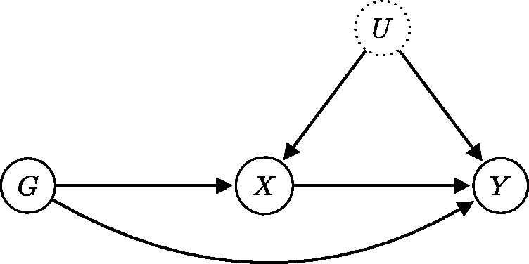
The application of MR methods requires genetic variants that are valid instruments for the exposure–outcome association, i.e. genetic variants satisfying the core IV assumptions. If a causal link from exposure to outcome exists, then a genetic variant associated with the exposure will also be associated with the outcome. Under the core IV assumptions, the converse also holds: an association between the genetic variant and the outcome implies the existence of a causal link from the exposure to the outcome. When these assumptions are violated, however, we can no longer be sure that a causal link from exposure to the outcome exists. A discovered genetic association with the disease outcome could be produced via a different causal pathway which is not mediated by the exposure (see Figure 6). In this case, the bias in the causal effect estimate obtained through the MR approach is potentially unbounded.
22
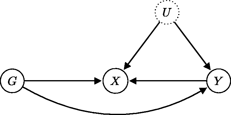
Even worse, if we are dealing with reverse causation for the exposure–outcome association, then the causal link whose effect we are trying to estimate does not exist (see Figure 7).
The local causal discovery
23
(LCD) pattern can be discovered from observational data by testing if the genetic variant G is independent from the outcome Y when conditioning on the exposure X. The genetic variant G is pleiotropic since it affects both phenotypic measures (X and Y). In this illustration, G exhibits both vertical pleiotropy (X and Y are influenced by G via the same causal pathway Reverse causation refers to the situation when the outcome Y precedes and causes the exposure X instead of the other way around.
48
The term “reverse” refers to the fact that the direction of the causal effect is opposite to what was expected based on the study design. We emphasize that although we denote the exposure by X and the outcome by Y, these terms do not have any causal meaning, i.e. they do not imply a particular causal ordering.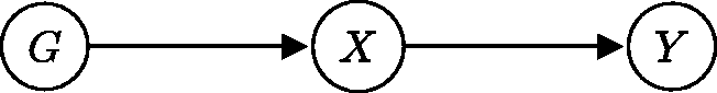
Unfortunately, only assumption IV1 is directly testable from data. It is typically fulfilled by selecting only those genetic variants that are associated with an exposure of interest. In general, the validity of assumptions IV2 and IV3 cannot be established from the data, since they involve the unobserved confounder U.
15
However, if the exposure–outcome association is unconfounded (see Figure 5), then we can check the validity of IV2 and IV3 by performing a conditional independence test. In this particular scenario, the genetic variant becomes independent of the disease outcome after conditioning on the exposure variable. This principle of testing the IV assumptions by looking for a conditional independence is used to orient the causal relationship between the two traits in mediation-based approaches
24
such as the likelihood-based causality model selection,
25
the regression-based causal inference test,
26
or the
Assumption IV2 is not completely testable since there can always be unmeasured confounding variables for which we cannot account, but we can at least filter out the genetic variants associated with any potential confounding traits that have been measured. 29 Fortunately, it is not very likely that genetic variants are associated with confounders of the exposure–outcome association. 30 The assumption that is most likely to be violated is IV3, which states that the instrumental variable is only related to the outcome via its effect on the risk factor. 31 Assumption IV3 does not hold if there are alternative causal pathways between the genetic variant and the disease outcome that are not mediated by the exposure (see Figure 6). This often happens when a genetic variant influences more than one phenotypic traits, a property called pleiotropy. 32
As the GWAS sample sizes continue to grow, the number of candidate genetic variants to be used as potential instruments is also increasing. Unfortunately, more and more of the supplied candidates are likely to be invalid instruments. Hemani et al. 33 show that horizontal pleiotropy and reverse causation can easily lead to invalid instrument selection in MR and suggest that the presence of horizontal pleiotropy should be considered the rule rather than the exception. This severely limits the application of MR to cases where previous background knowledge can be used to validate the core assumptions. By relaxing (some of) these assumptions, however, the MR approach can be applied to a much broader range of genetic variants.
2.3.1 Pleiotropy
In the genetics of complex diseases it is common for genetic variants to affect multiple disease-related phenotypes.34,35 If such a pleiotropic genetic variant affects the disease outcome through different causal pathways, then IV2 or IV3 or both are potentially violated. This makes pleiotropy problematic for MR studies.4,15 As a result, many recent extensions of the MR approach have been aimed at producing better causal estimates in the presence of pleiotropic effects.17,32,36–40 Pleiotropy can be divided into horizontal (biological) pleiotropy and vertical (mediated) pleiotropy. Horizontal pleiotropy occurs when the same genetic variant affects multiple trait via different biological pathways, whereas vertical pleiotropy occurs when the same genetic variant is associated with multiple traits found on the same biological pathway. We will only focus on the former, since only horizontal pleiotropy can lead to violations of IV3, and refer to it hereafter as “pleiotropy”, for brevity. 32
Two main approaches have been used for robustifying MR against potentially pleiotropic genetic variants. The first approach is to replace some of the (untestable) IV assumptions, e.g. IV2 or IV3 or both, with a weaker set of alternative assumptions. The second approach is to assume that the IV assumptions hold for some, but not necessarily for all the genetic variants. In this case, the invalid genetic instruments are allowed to violate the IV assumptions in an arbitrary way. 41
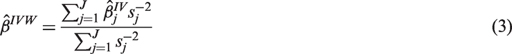
MR-Egger regression 17 is a pleiotropy-robust method that falls into the first category. MR-Egger is an extension to the IVW method introduced in Subsection 2.2, in which an intercept term is added to the weighted linear regression of the genetic associations with the outcome on the genetic associations with the exposure. While IVW is consistent if the pleiotropic effects average to zero across the genetic variants, this extension allows for consistency even when the pleiotropic effects do not average to zero. Both the IVW and MR-Egger methods work under the instrument strength independent of direct effect (InSIDE) assumption, which stipulates that the association with the exposure is independent from the direct (pleiotropic) effect on the outcome across different genetic variants. 41 Another robust alternative to the IVW estimator is the weighted median estimator 36 (WME), for which we compute a weighted median of the IV estimates instead of a weighted average. The WME is a consistent estimate of the true causal effect as long as at least 50% of the genetic instruments are valid. In a similar vein, Kang et al. 42 have introduced an LASSO 43 -type procedure to identify the valid instruments from within a set of candidate genetic variants. Hartwig et al. 37 have proposed instead to compute the weighted mode of the individual IV estimates to obtain the mode-based estimate (MBE). The MBE can be a consistent estimate of the true causal effect even when fewer than 50% of the genetic instruments are valid. However, the application of the method relies on the assumption that the largest number of similar individual IV estimates comes from valid instruments, an assumption termed the Zero Modal Pleiotropy Assumption (ZEMPA). Finally, Hemani et al. 33 suggest combining these methods (along with others) in a “mixture of experts” machine learning approach. 44
A number of Bayesian modeling approaches for dealing with pleiotropic genetic variants have been proposed, in which all variants used as instruments are allowed to exhibit pleiotropic effects on the outcome. Li 38 introduced empirical Bayes hierarchical models for estimating the causal effect in MR studies where many instruments are invalid, while Berzuini et al. 40 performed a fully Bayesian treatment of the MR problem. In both cases, the authors handled pleiotropy by putting shrinkage priors on the pleiotropic effects, thereby forcing them to take values close to zero unless there is strong posterior evidence for pleiotropy. 45 Thompson et al., 46 on the other hand, modeled pleiotropy explicitly and used Bayesian model averaging to provide estimates that allow for uncertainty regarding the nature of pleiotropy.
2.3.2 Reverse causation
A crucial aspect that is often overlooked in MR studies is the implicit assumption made regarding the direction of the causal link between the exposure and the outcome. While it is sometimes possible to rule out reverse causation, in most situations there is not enough background knowledge available about the underlying causal mechanism. The observed relationship between low levels of LDL cholesterol and risk of cancer is an example where we cannot a priori assume a causal direction. It may be that low levels of LDL cholesterol are causal for cancer, but it is also possible that the presence of the disease has a negative effect on LDL cholesterol. 5 In the case of complex systems such as gene regulatory networks, it is also unclear in which direction the gene regulation occurs. 47
The existence of alternative causal paths from a genetic variant to the outcome of interest affects not only the estimation of causal effects but also model identification. If there exists a causal pathway from the genetic variant to the outcome that is not mediated by the exposure, then an exposure–outcome causal link is no longer required to explain their association (see Figure 6). In fact, the causal link between the two traits may have the opposite direction (see Figure 7). Ignoring the possibility of reverse causation for the exposure–outcome association is potentially dangerous. If the true causal link is in the expected direction (from X to Y, Figure 6), we will be underestimating the uncertainty of our estimate by not considering the alternative model. If the true causal link is in the opposite direction (from Y to X, Figure 7), then the MR approach will produce a misleading result, as we are trying to estimate the wrong causal effect. Bidirectional MR
4
is one approach used to distinguish between an “exposure” having a causal effect on an “outcome” and the reverse. The idea is to perform MR in both directions to tease apart the causal relationships
Agakov et al.
49
proposed a Bayesian framework built on sparse linear methods developed for regression, which is similar in spirit to
2.4 Summary
MR is a powerful principle that can help strengthen causal inference by combining observational data with genetic knowledge. However, MR methods require good candidate genetic variants to be used as instruments, which often limits their application to variants with well understood biology. The wide spread of pleiotropic genetic variants, which violate key IV assumptions (IV2 and especially IV3), is a particularly troublesome issue.4,52 Many methods have been designed to improve causal effect estimation in the presence of pleiotropic effects,38,40,46 but they do not incorporate the possibility of reverse causation. At the same time, a number of methods have been developed for inferring the correct direction of the causal link between two phenotypes,24,33 but these do not provide a measure of uncertainty in the model selection. In the following section, we introduce a general method with which we aim to handle all of these issues simultaneously. We first perform Bayesian model averaging to account for the uncertainty in the direction of the causal link and then, for each model, we obtain an informative posterior distribution for the causal effect of interest.
3 Bayesian model specification
3.1 Setup
We assume that the data are generated from the model illustrated in the causal diagram from Figure 8, where all relationships between variables are linear with no effect modification. We consider J independent genetic variables, which we denote by Graphical description of our assumed generative model. We denote the exposure variable by X and the outcome variable by Y. We are interested in the causal effect from X to Y, which is denoted by β. The association between X and Y is obfuscated by the unobserved variable U, which we use to model unmeasured confounding explicitly. The shaded plate indicates replication across the J independent genetic variants 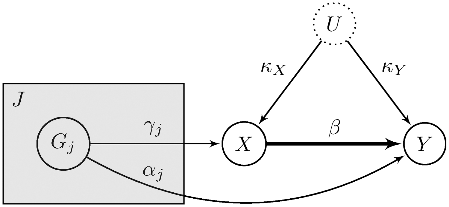
The generative model from Figure 8 is described by the following linear structural equation system

In this work, we restrict our attention to the case where the exposure and outcome variables are continuous. We also assume without loss of generality that
3.2 Model assumptions
The first two core IV assumptions are implied by our proposed model. The existence of direct edges from each Gj to the exposure X implies that IV1 is satisfied for each genetic variant. At the same time, we assume that for any
In our model, we assume that the instrument strengths
We also assume that the genetic variants are independent, i.e.
3.3 Likelihood
We assume that the data generating process is described by equation system (4) and that each data sample is a complete set of observed values for the exposure X, the outcome Y and the genetic variants
We collect all parameters of the model in the vector
We model each genetic variable Gj as binomially distributed, where we count the number of effect alleles at the genetic locus, either 0, 1, or 2. If pj is the EAF of Gj, then the binomial distribution has parameters n = 2 and

Given the conditional linear-Gaussian model, the log-likelihood is equal, up to constant terms, to

3.4 Priors
According to Jones et al., 56 informative priors are crucial to the success of Bayesian MR methods, regardless of whether or not they are identifiable, and the so-called “vague” (uninformative) priors should be avoided whenever possible. Thompson et al. 46 mention two arguments against the use of an uninformative prior in the MR context: (1) that the analysis is already subjective due to the selection of the genetic variants and (2) the data alone are sufficient to produce useful estimates of the causal effect. However, care must be taken when specifying informative priors, as substantial variation in parameter estimates can occur as the prescribed priors are modified.
For most genetic variants, it is unrealistic to expect exactly zero pleiotropy, i.e. that the effect on the outcome variable is completely mediated by the exposure.
57
However, we can differentiate between pleiotropic effects that are weak and strong relative to the other interactions. A weak pleiotropic effect will not introduce significant bias, and therefore still enable us to produce a useful estimate of the causal effect, in spite of the violation of IV3.
58
For this reason, in choosing the prior for our structural parameters, we start from the assumption that the interactions between variables are either “strong” (relevant) or “weak” (irrelevant), in a similar vein to the considerations made by Berzuini et al.
40
This is different from the standard assumption that the pleiotropic effects are either zero or nonzero as used, for example, in the LASSO-based method of Kang et al.
42
A reasonable choice for the prior (of

Our Gaussian mixture prior induces model parsimony by giving a preference for the model with the smallest number of strong parameters, which will then allow us to choose the most parsimonious causal explanation (direct causation, reverse causation, no causation). 61 Moreover, since every interaction is shrunk selectively, in the sense that smaller coefficient estimates are shrunk towards zero more sharply than larger coefficients, a significant gain in efficiency can be achieved. 62 Other shrinkage priors, such as the horseshoe employed by Berzuini et al., 40 have also been used successfully for Bayesian MR. However, we have chosen the spike-and-slab prior due to ease of implementation and interpretation. In our experiments, we found that nested sampling works better when we specify the structural parameter (marginal) prior density directly instead of using a hierarchical approach. Consequently, we found it is helpful that the spike-and-slab prior density is simply a mixture of Gaussian densities, as opposed to the horseshoe prior density which has no closed-form expression. 63
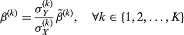
3.4.1 Rescaling
To make our method independent of the measured variables’ scale, we rescale our model parameters as follows. We divide the first equation in equation (4) by

The standardized variables

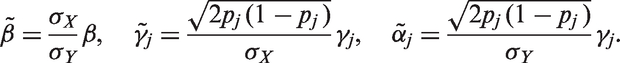
We then put priors on the set of rescaled parameters
3.4.2 Choice of priors
3.4.3 Prior hyperparameters
When we do not know if the (potentially pleiotropic) genetic variants we intend to use for MR are valid or not, it is unclear whether their pleiotropic effects are more likely to be “large” or “small”. To express this uncertainty, we define the hyperparameter
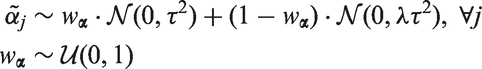
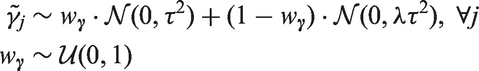
We can make a similar argument for the strength of the association between the genetic variants and the exposures, i.e. the “instrument strengths”. Analogously, we obtain the hierarchical prior
4 Bayesian model averaging and inference
4.1 Computing the model evidence
The Bayesian view of model comparison involves the use of probabilities to represent uncertainty in the choice of model.
44
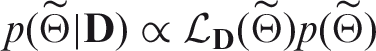
We define the prior probability of a model


The model evidence can be viewed as the probability of generating the data set
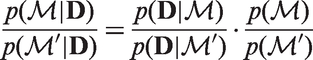
When performing model comparison, it is convenient to work with probability ratios. The prior odds ratio
In our approach, we compare two competing models corresponding to the two possible causal orderings for the non-genetic variables: Competing models encompassing both possible directions for the causal link between exposure and outcome. (a) 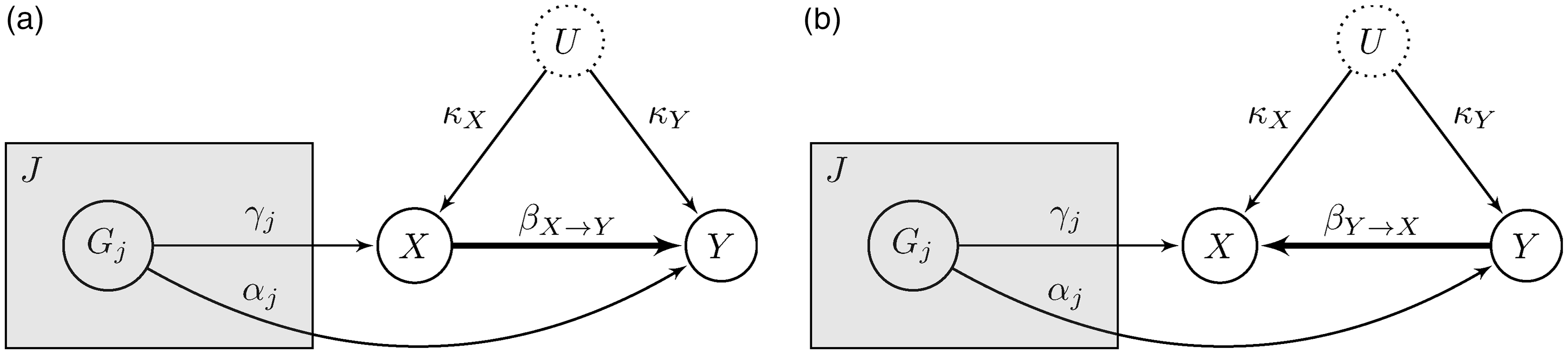
The marginal likelihood for these models is also difficult to compute, with the Gaussian mixture prior on the parameters leading to a multimodal posterior. To solve our problem, we have used the
If we have background knowledge that can be used to express a prior preference for one of the two models, we can easily incorporate it into our framework. We simply have to change the prior probabilities for each model. For example, if we know that X precedes Y temporally, we can eliminate the possibility of reverse causation. In that case,
4.2 Posterior inference
We take as input the complete data set of N i.i.d. observations
The Bayesian inference process is described in Figure 10 for the expected direction of the causal link. For the reverse direction, we simply switch the positions of X and Y. Given our choice of prior distributions for the rescaled parameters (see Subsection 3.4), we draw K samples from the full posterior distribution
Compact description of the Bayesian inference process using plate notation. The small rectangles indicate our model parameters, while the circles denote random variables (observed or unobserved). The gray superposed areas signify replication across the J genetic variants and the N data points. This is also suggested by the subscripts used for parameters and variables.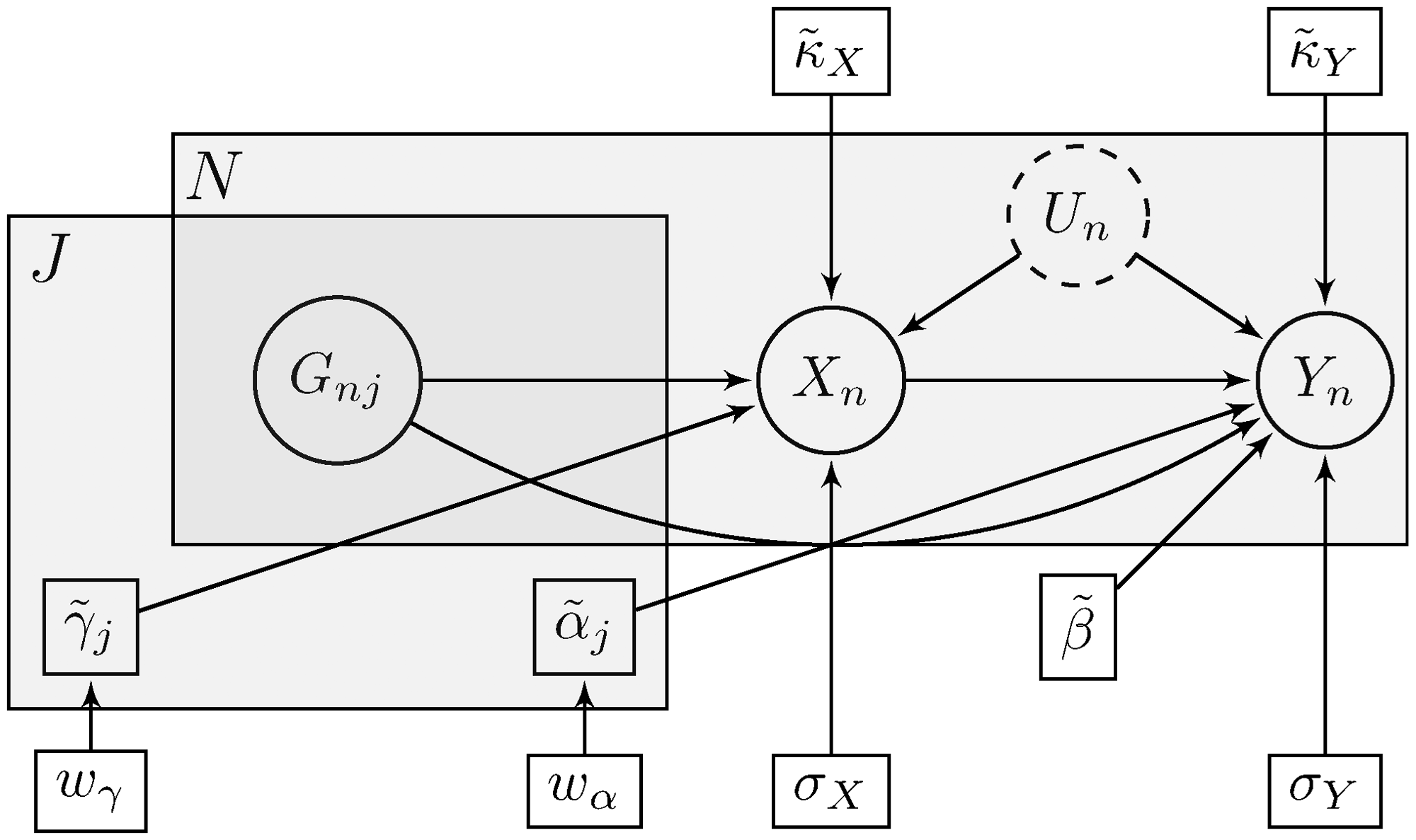
Finally, we compute the evidence for both directions, i.e.

4.3 Example: Instrumental variable setting
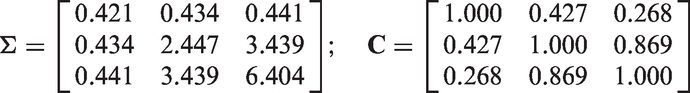
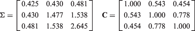
We first consider a simple generating instrumental variable model with one genetic instrument (see Figure 11) to illustrate the model comparison and averaging procedure. In this example, the instrument strength γ, the causal effect β, and the confounding effect Generating model where the causal relationship is from X to Y (the expected direction). This model satisfies all three instrumental variable assumptions.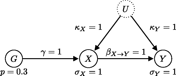
We now fit models
This result is perhaps surprising at first glance, as it implies that there is at least a one in three chance that the causal relationship is in the reverse direction. However, when we allow for pleiotropy, it becomes possible to fit a similarly sparse model where the Alternative generating model, statistically equivalent to the one in Figure 11, where the causal relationship is from Y to X (the reverse direction).
4.4 Example: Near-conditional independence (near-LCD)
We now look at an example where the confounding and pleiotropic effects are weak relative to the instrument strength and to the exposure–outcome causal effect. The generating model is depicted in Figure 13. We call this example near-LCD, because if we made the confounding and pleiotropic effects infinitely weak, i.e. Generating model where the causal relationship is from X to Y (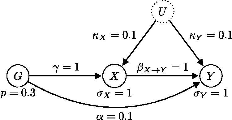
For the prior hyperparameters Estimated posterior density of the causal effect 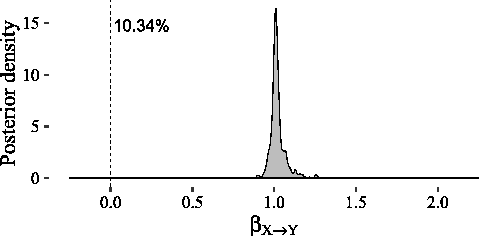
5 Simulation studies
5.1 Estimation robustness
We imagined a typical MR scenario where there are a number (J = 25) of genetic variants that may be used as instruments, but it is not known how many of them satisfy the IV assumptions. We analyzed the robustness of the causal effect estimate produced by our method to the presence of pleiotropy. We first treated the case where all variants were valid instruments. We then added pleiotropic effects to the genetic variants, such that only 80%, 60%, 40%, 20%, and finally 0% of them were valid instruments. We generated data according to the Bayesian model specification in Section 3 (see Figure 8). The EAF of each genetic variant were randomly simulated from a uniform distribution. We simulated the instrument strengths (
For the inference, we set the prior hyperparameters to The effect of introducing pleiotropic effects on the posterior estimates is that the distribution moves away from the true value 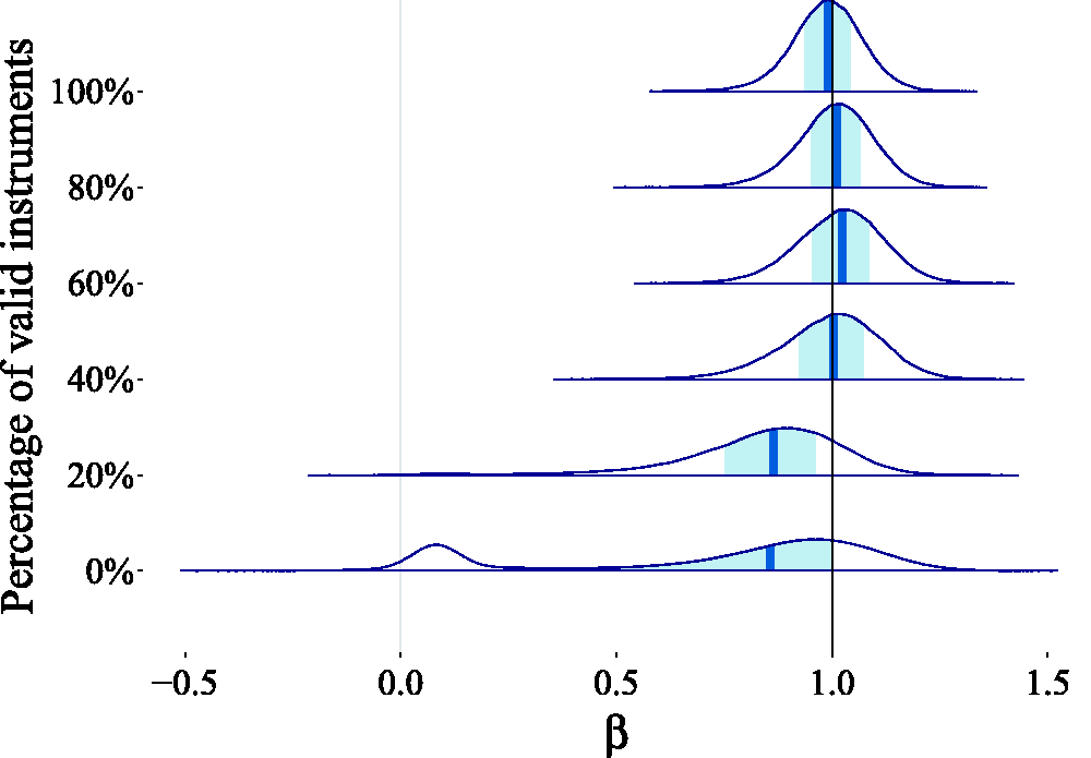
5.2 Sensitivity to prior hyperparameters
In this simulation, we analyzed how the posterior computed by Posterior distribution of β for different hyperparameter settings (only λ is varied) in the near-LCD scenario (Figure 13). The true value for β is depicted by a dashed vertical line.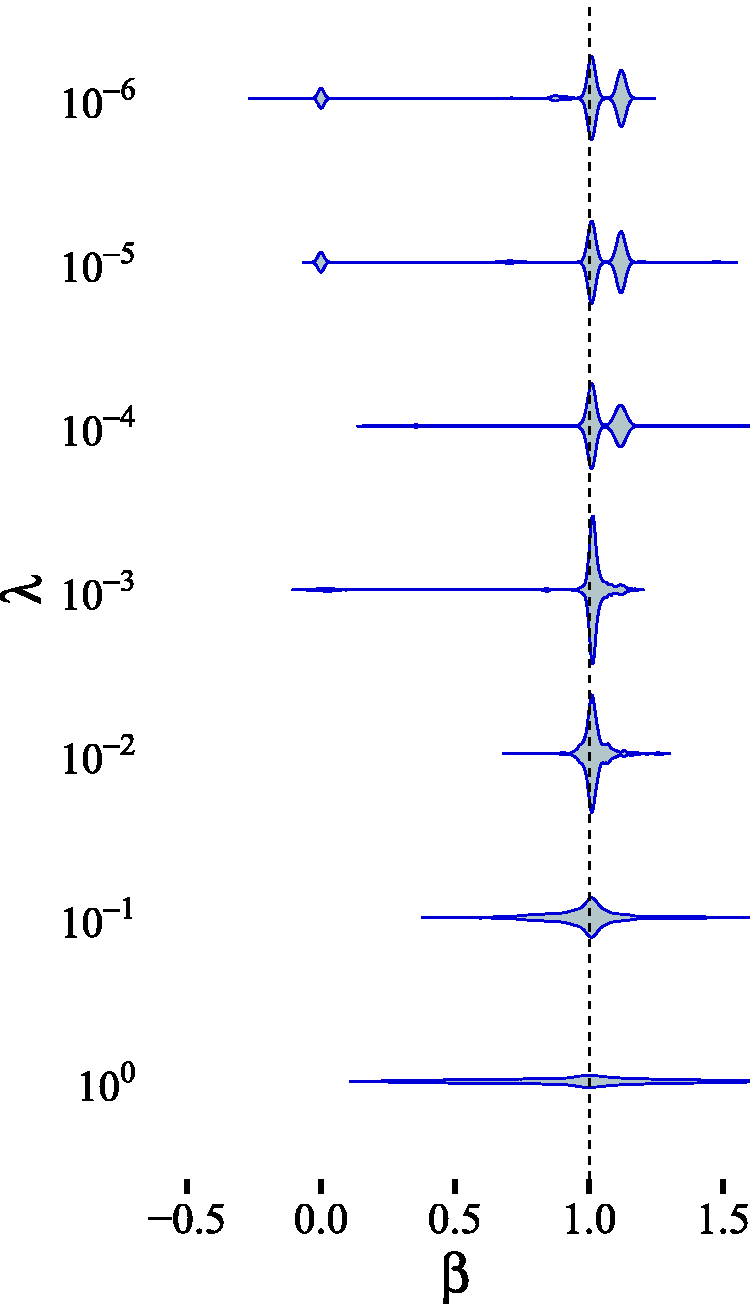
The obtained posterior is sensitive to the hyperparameter choice, as reflected by the different mode heights in the multimodal posterior. This is due to the fact that the prior incorporates our belief regarding the magnitude of “weak” and “strong” effects. For instance, the appearance of the second mode around 1.1 for smaller values of λ can be explained by the change in the prior belief that the pleiotropic effect, which is of magnitude
Even though, as we have shown, the posterior distribution is driven by the choice of prior hyperparameters, our approach also enables the researcher to easily incorporate useful background knowledge, such as previously established weak or strong interactions, into the system. The advantage lies in the intuitive interpretation of the hyperparameters for the Gaussian mixture prior (see Subsection 3.4).
5.3 Model averaging robustness
In this experiment, we considered a bidirectional MR setting (see Subsection 2.3.2), where we cannot exclude the presence of pleiotropic effects. For simplicity, we considered a single genetic variant GX known to be associated with X and a single genetic variant GY associated with Y. The true causal direction in the generating model was from X to Y. This generating model is described by the set of equations

In our simulation, the genetic variants were strongly associated with their respective phenotypes:
The results of performing a simple bidirectional Mendelian randomization analysis for various degrees of pleiotropy.
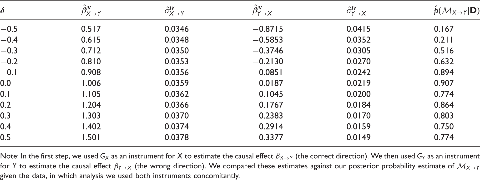
Note: In the first step, we used GX as an instrument for X to estimate the causal effect
In the presence of pleiotropic effects (
5.4 Sensitivity to nonlinearity and nonnormality
Our assumed Bayesian model, as described in Section 3, entails a linear relationship between the exposure X and the outcome Y, as well as a conditional Gaussian distribution given the instrument values,
The results of running
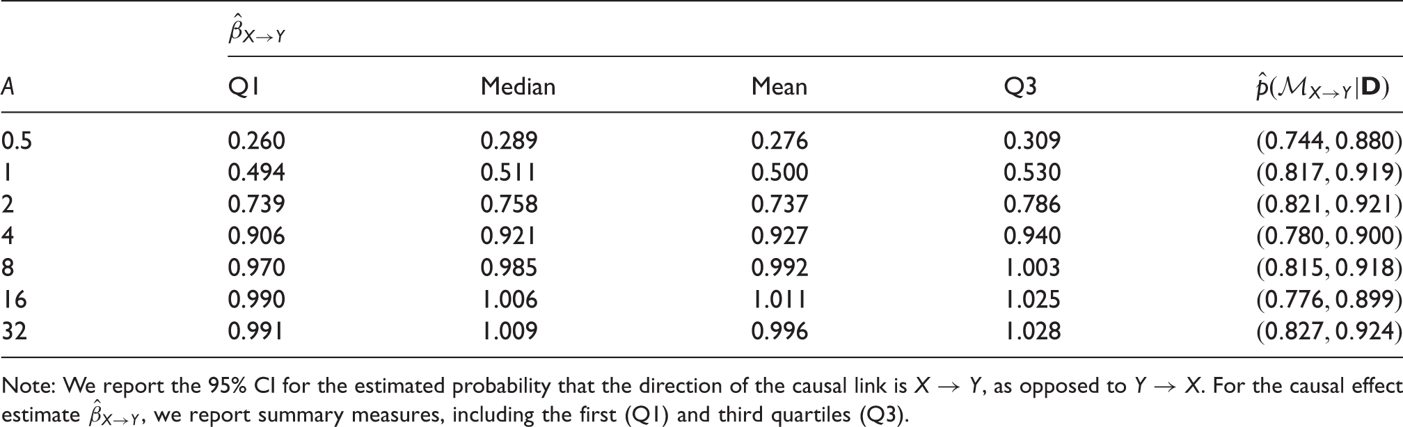
Note: We report the 95% CI for the estimated probability that the direction of the causal link is
The results of running
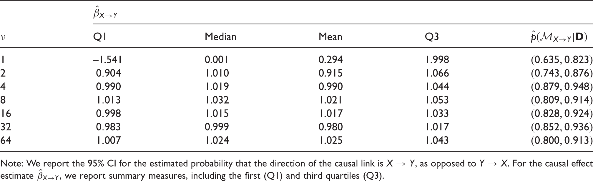
Note: We report the 95% CI for the estimated probability that the direction of the causal link is
6 Real-world applications
In this section, we will showcase the potential of
6.1 Using summary data
m: the number of allele copies (very often equal to two, since humans are diploid organisms)
Summary data on gene-exposure and gene-outcome associations from GWAS has become increasingly available, so we can typically get estimates for
To derive the expected values and variances for the genetic variants, we employ the binomial distribution assumption by plugging in the EAF as the estimated success probability and using the appropriate formulas. We can assume without loss of generality that the mean parameters 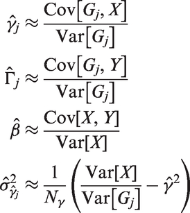
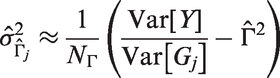
Note that these approximations also apply in a multivariate setting when the regressors are independent. We use these approximations to finally derive the following estimates for the moments from summary statistics
When we have information on multiple genetic variants, we obtain multiple estimates of
6.2 Effect of birth weight on fasting glucose
Del Greco et al. 71 performed an IVW meta-analysis of MR Wald estimates (see equations (2), (3)) to analyze the relationship between low birth weight and adult fasting glucose levels. The authors chose seven genetic variants associated with birth weight to use as instruments in an MR analysis. The meta-analysis of the seven MR estimates suggested a significant protective effect of −0.155 mmol/L (95% CI (−0.233, −0.088)) reduction in adult fasting glucose level per standard deviation increase (484 g) in birth weight. In their analysis, Del Greco et al. 71 investigated the presence of pleiotropy by means of the between-instrument heterogeneity Q test. They reported significant evidence of heterogeneity across instruments (p = 0.03), which they believe suggests that IV3 might be violated for some of the genetic variants. The heterogeneity was primarily due to the variant rs9883024 in gene ADCY5. However, even after removing said variant from the analysis, they obtained a significant negative effect estimate of −0.098 (95% CI (−0.168, −0.027)).
We ran our model using the summary statistics for the genotype-exposure and genotype-outcome associations provided in Table IV of Del Greco et al. 71 . The regression coefficient for the observational exposure–outcome association is taken from Daly et al., 72 who reported a decrease of 0.01 mmol/L in fasting glucose levels per kilogram increase in birth weight in a retrospective cohort study on a multiethnic sample of 855 New Zealand adolescents. The regression coefficients they computed were adjusted for age, sex, and ethnicity. One potential limitation of using this data is that there may be biases induced by the different adjustments made in the study. 31 Another potential issue is the fact that the observational study sample is taken from an underlying population which is different in terms of ethnicity and age. 73 Nevertheless, the associations found in the observational study are consistent with those found in subsequent studies. 74
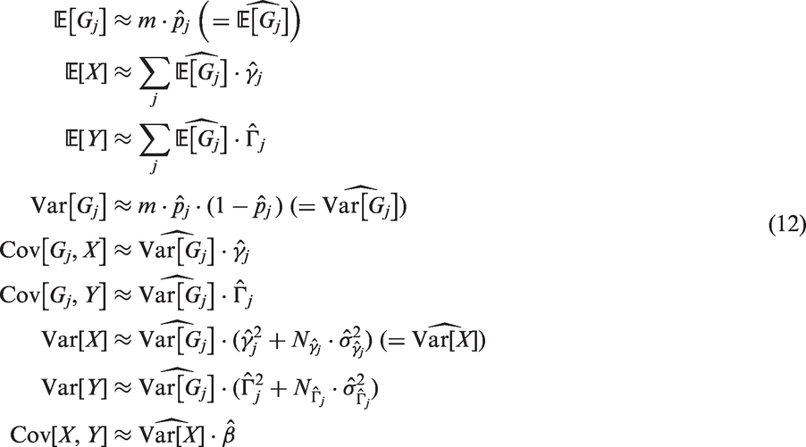
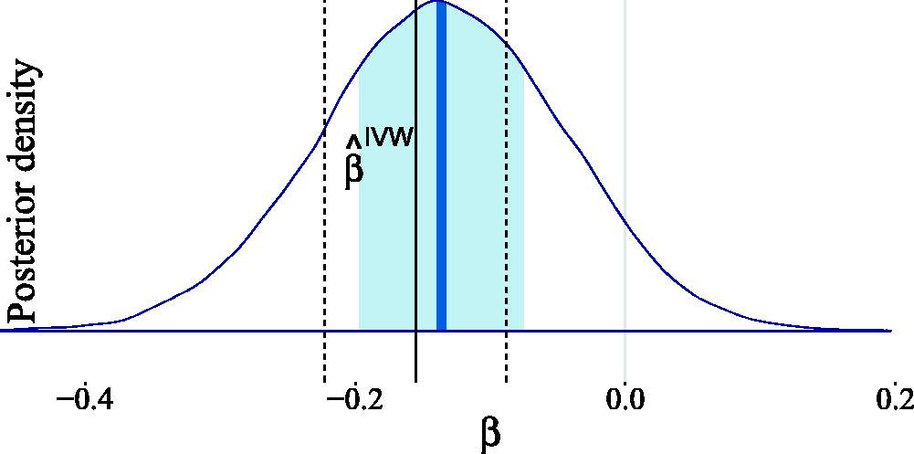
Our estimated posterior in Figure 17 indicates that no causal effect is necessary to explain the observed data. This conclusion differs significantly from that of Del Greco et al.
71
because we are making less stringent assumptions regarding the parameter strengths. However, we can arrive at their conclusion if we adapt our prior knowledge by incorporating stronger prior assumptions. To obtain the posterior distribution in Figure 18, we assumed that the pleiotropic effects are negligible (by setting Estimated posterior distribution for the causal effect of birth weight on adult fasting glucose levels. The light shaded area in the posterior represents the interquartile range, while the dark shaded line indicates the median. For the Gaussian mixture prior in equation (7), we have taken Estimated posterior distribution for the causal effect of birth weight on adult fasting glucose after adapting the prior knowledge to fit the classic instrumental variable setting. The light shaded area in the posterior represents the interquartile range, while the dark shaded line indicates the median. For the Gaussian mixture prior in equation (7), we have taken 
6.3 Effect of BMI on the risk of PD
There have been conflicting findings regarding the association between BMI and PD in observational studies. Both positive and negative associations between higher BMI and the risk of PD have been reported. 75 Wang et al. 76 performed a meta-analysis of 10 cohort studies and their obtained pooled risk ratio (RR) for the association of a 5 kg/m2 higher BMI with the risk of PD was 1.00 (95% CI (0.89, 1.12)), which suggests that BMI is not associated with the risk of PD. In an MR analysis, Noyce et al. 75 estimated the causal effect of BMI on the risk of PD by combining the ratio estimates corresponding to 77 selected single-nucleotide polymorphisms (SNPs) via an IVW scheme. The results of their analysis suggest a putative protective causal effect of BMI. More specifically, their MR analysis yielded an IVW log-odds ratio (log-OR) of −0.195 (95% CI (−0.368, −0.021)), meaning that a lifetime exposure of 5 kg/m2 higher BMI was associated with a lower risk of PD.
We also took the log-OR as the continuous outcome variable. We used the summary data from Noyce et al.
75
for the genetic associations with BMI and the log-OR of PD. We used the RR reported by Wang et al.
76
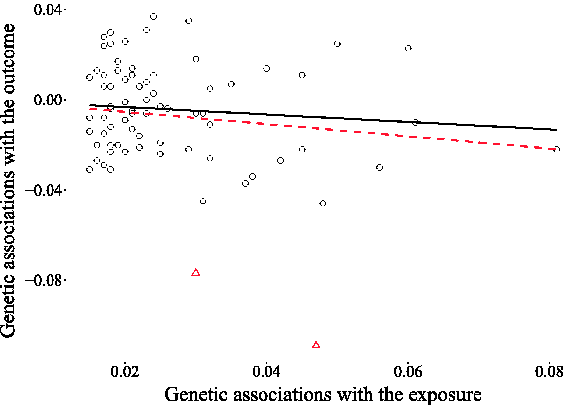
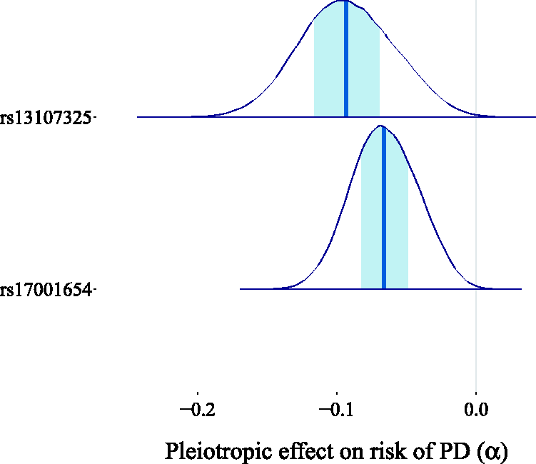
as an approximation for the OR, since the incidence of PD is very low, resulting in an estimated log-OR of zero for the observational association of a 5 kg/m2 higher BMI with the risk of PD. We fitted our model assuming the direction of causality from BMI to PD and we obtained a causal effect estimate centered around zero, with 96.3% of the probability mass in the interval (−0.1, 0.1) (see Figure 19). This result casts doubt on the existence of a causal link between BMI and the risk of PD. When looking at the scatter plot comparing the genetic associations of the 77 variants with the outcomes and their associations with the exposures (Figure 20), we observe the existence of two outliers, corresponding to the red triangles. These two variants show a low association with the outcome relative to the others given their strength as instruments. It is possible that the unusually large negative association with the risk of PD is due to unobserved pleiotropic effects. This claim is supported by our estimates of the pleiotropic effect α for these two genetic variants, which are shown in Figure 21.
Estimated causal effect of BMI on the risk of PD expressed as the difference in log-odds of PD per 5 kg/m2 increase in BMI. The light shaded area in the posterior represents the interquartile range, while the dark shaded line indicates the median. The IVW estimate Scatter plot of the genetic associations with BMI (horizontal axis) and PD risk (vertical axis) for 77 genetic variants. The two outliers (triangles) show a relatively strong association with the outcome given their association with the exposure. The regression line including the outliers is dashed, while the regression line obtained without the outliers is continuous. Estimated pleiotropic effects for the two genetic variants suspected of being pleiotropic outliers (rs17001654 and rs13107325). The light shaded area in the posterior represents the interquartile range, while the dark shaded line indicates the median. Most of the posterior mass is distributed away from zero, thereby supporting the suspicion that these two variants exhibit horizontal pleiotropy.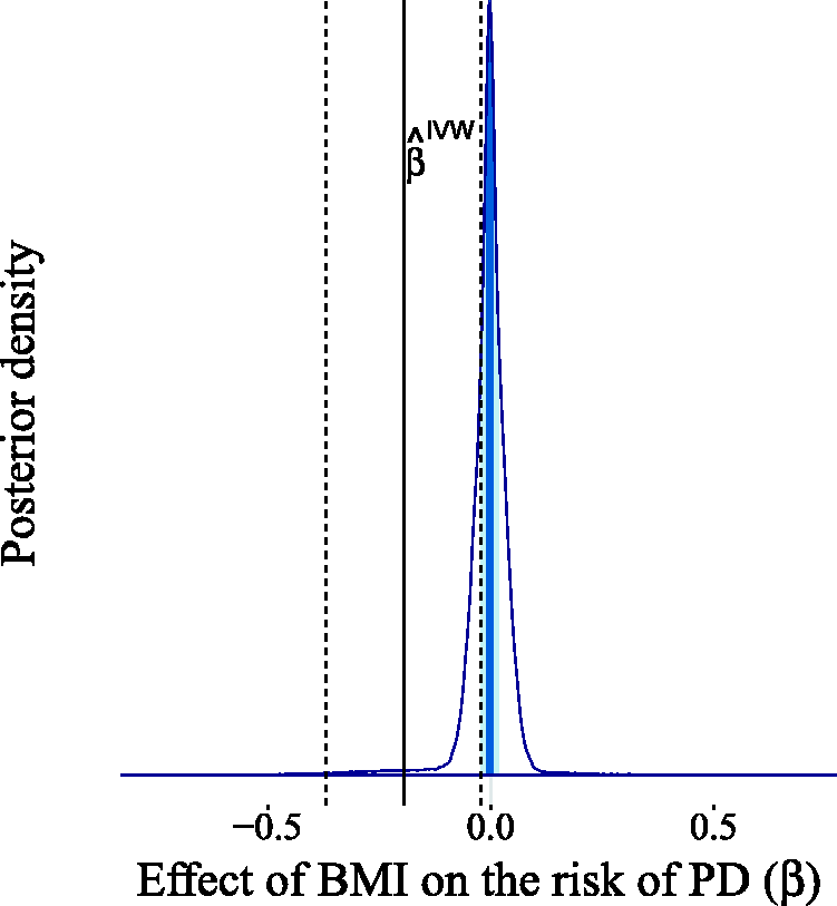
To further substantiate our claim that these variants represent outliers for the IVW and MR-Egger analysis, we used the radial regression approach of Bowden et al.
77
By running the radial IVW and MR-Egger regressions using first-order weights and specifying a statistical significance threshold of 0.01, we discovered the same two outliers observed visually in the scatter plot. Alternatively, we used the MR pleiotropy residual sum and outlier (MR-PRESSO) test
57
to identify potential pleiotropic outliers. With MR-PRESSO, we detected the two genetic variants highlighted in Figure 20 as outliers for a significance threshold of 0.1. The outlier-corrected causal estimate produced by MR-PRESSO remained “barely” significant at the 0.05 level:
To sum up, the results of our investigation suggest that the protective causal effect of BMI on the risk of PD discovered by Noyce et al. 74 could also be due to some of the genetic variants exhibiting horizontal pleiotropy. We suspect two variants in particular to be pleiotropic outliers in the MR analysis, as suggested by our method and other approaches.57,77
6.4 Does coffee consumption influence smoking?
In this experiment, we investigated the association between coffee consumption and cigarette smoking. It is unclear whether this association is causal. An MR study performed by Treur et al. 78 provided no evidence for causal effects of smoking on caffeine or vice versa. Bjørngaard et al., 79 on the other hand, found that higher cigarette consumption causally increases coffee intake. If a causal link between coffee consumption and cigarette smoking exists, its direction is also unclear. Verweij et al. 54 employed a two-sample bidirectional MR study to investigate, among other things, the causal association between the use of nicotine and caffeine, but found little evidence of a causal relationship in either direction. In another study, Ware et al. 80 assessed the impact of coffee consumption on the heaviness of smoking, but also obtained inconclusive results: one of their two-sample MR analyses indicated that heavier consumption of caffeine might lead to reduced heaviness of smoking, while in other MR analyses they found no evidence of a causal relationship between coffee consumption and heaviness of smoking. Ware et al. 80 concluded it is unlikely that coffee consumption has a major causal impact on cigarette smoking and suggested the possibility of reverse causation, i.e. smoking impacting coffee consumption, or confounding as alternative explanations for the observed association.
We used the summary statistics reported by Ware et al.
80
to explore this association. The exposure variable is coffee consumption measured in cups per day, while the outcome variable is smoking measured in cigarettes per day. The summary measurements for the gene-exposure association were taken from the European replication sample (
In our approach, we considered two candidate models corresponding to the two possible causal directions. In the first model (Figure 6), we assumed a causal link from coffee consumption to smoking, while in the second model (Figure 7), we assumed the reverse causal link. We computed the evidence for the two models and then, assuming a priori that either of the two models is equally likely, we obtained a posterior probability of 42.6% for the first model and 57.4% for the second model. The posterior over the causal effect is shown for both directions in Figure 22(a) and (b). According to our results, there is significant uncertainty in the direction of the causal effect. This suggests that the observed association may in fact be due to some confounding factor. Still, that does not exclude the possibility of a causal effect between coffee consumption and heaviness of smoking, but more data are required to substantiate this claim.
Comparison of the causal effect estimates between X (coffee consumption in cups per day) and Y (heaviness of smoking in cigarettes per day) for the two possible causal directions. The estimated evidence for the two models is 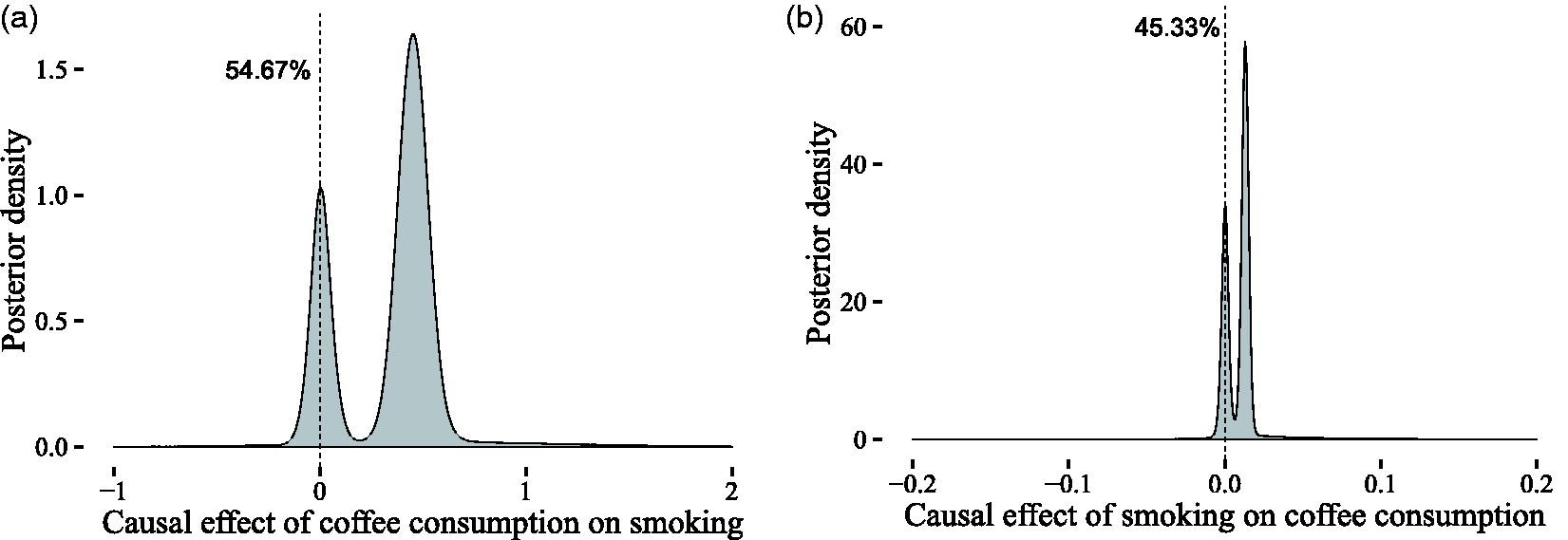
7 Discussion
In this paper, we have proposed a
Many traditional MR methods can be seen as limiting cases of our more general approach. For example, the “no pleiotropy” assumption
68
made when using genetic variants as instrumental variables can be incorporated by setting the prior proportion of the slab component for the pleiotropic effect to zero (
In the era of high-throughput genomics, it is becoming increasingly likely to select invalid instruments as GWAS sample sizes continue to grow.
33
Our approach allows for the selection of a much broader range of genetic variants, since it does not require any of the instruments to be valid. Furthermore, we can select even those variants for which it is not clear whether they primarily influence the exposure or the outcome. In this sense, we envision running
A key aspect of our approach lies in the structural assumption that interactions between variables are either “weak” (irrelevant) or “strong” (relevant).
61
This assumption is different from the traditional zero–nonzero dichotomy and, in our opinion, more realistic than assuming, for example, that a genetic effect on an outcome variable is “completely mediated” by another variable. The Gaussian mixture prior is a natural choice for expressing this assumption and has the intuitive interpretation of capturing the small, irrelevant effects in the “spike” (lower variance) component and the large, relevant effects in the “slab” (higher variance) component. The mixture Gaussian prior has already been used, for example, by Li
38
to induce sparsity in the estimation of pleiotropic effects. Here, we extend the usage of this prior to the other structural parameters, which allows for a more general view of MR analyses. For example, putting a Gaussian mixture prior on the strength of instruments will enable us to make an automatic selection of the relevant instruments in a batch of preselected genetic variants, where the proportion of relevant instruments can be determined by learning the shared hyperparameter
Our chosen prior is informative in the sense that it informs which effects we consider a priori to be relevant. Because of this, care must be taken when setting the prior hyperparameters. While this informativeness may be seen as a weakness of the Bayesian approach, it also empowers the research to input sensible assumptions regarding the expected magnitude of effects in an intuitive fashion. If one has a prior idea regarding which effect sizes are deemed relevant and which irrelevant, then one can appropriately tune the variances of the “spike” and the “slab” to reflect this belief. When it is not clear how to distinguish between relevant and irrelevant effects, one can treat all detectable effects as relevant by letting
One important limitation of the approach proposed here lies in the strong parametric assumptions of linearity and Gaussianity.
15
These standard assumptions are commonly made for simplicity and computational convenience in similar works such as those by Thompson et al.,
46
Li,
38
or Berzuini et al.,
40
but when they do not hold, the estimands can potentially be far off the mark and their interpretation is rendered incorrect. We have shown that
For future work, we plan to make our approach even more general by relaxing the IV2 assumption, and therefore taking into account the possibility that the genetic variables might be associated with unmeasured confounders. This would also mean that the InSIDE assumption, which is required for applying MR-Egger
17
or the Bayesian method proposed by Berzuini et al.,
40
does not hold. Another immediate extension to our work is handling potential measurement error for the exposure and outcome variables. Traditional methods such as MR-Egger rely on having no measurement error in the exposure (the so-called NOME
83
assumption), which is difficult to achieve in practical applications and may lead to erroneous results. Finally, we are also interested in analyzing the links between variables that exert a mutual causal influence on each other. For this purpose, we intend to extend
The code implementing the proposed method will be made publicly available by the authors at https://github.com/igbucur/BayesMR.
Footnotes
Acknowledgements
We would like to thank the anonymous reviewers for their thoughtful comments and efforts towards improving our manuscript.
Declaration of conflicting interests
The author(s) declared no potential conflicts of interest with respect to the research, authorship, and/or publication of this article.
Funding
The author(s) received financial support for the research, authorship, and/or publication of this article: This research has been partially financed by the Netherlands Organisation for Scientific Research (NWO), under project 617.001.451.