
Abstract
Diagnostic accuracy studies assess the sensitivity and specificity of a new index test in relation to an established comparator or the reference standard. The development and selection of the index test are usually assumed to be conducted prior to the accuracy study. In practice, this is often violated, for instance, if the choice of the (apparently) best biomarker, model or cutpoint is based on the same data that is used later for validation purposes. In this work, we investigate several multiple comparison procedures which provide family-wise error rate control for the emerging multiple testing problem. Due to the nature of the co-primary hypothesis problem, conventional approaches for multiplicity adjustment are too conservative for the specific problem and thus need to be adapted. In an extensive simulation study, five multiple comparison procedures are compared with regard to statistical error rates in least-favourable and realistic scenarios. This covers parametric and non-parametric methods and one Bayesian approach. All methods have been implemented in the new open-source R package
Introduction
The aim of diagnostic and prognostic studies is generally to differentiate between two groups, for example, the diseased from the non-diseased or those with good outcome from those with poor outcome. This differentiation can be based on a single clinical parameter or a combination of parameters. The methods and results presented here are independent of whether the goal is diagnosis or prognosis and whether a single parameter or a combination is evaluated. Furthermore, this work also covers the scenario that several investigated diagnostic procedures are defined by different (machine-learned) prediction models which are based on the same input data, for example, medical images. For better readability, the terms diagnosis, diagnostic study and diagnostic test are used in the following, but prognosis, prognosis study and prognostic marker are meant at the same time.
In order to assess the accuracy of a new diagnostic test, the so-called index test, the result is compared with the true condition, which is assessed using the gold standard or reference standard. The recommended co-primary endpoints are sensitivity as the proportion correctly diagnosed as diseased and specificity as the proportion correctly diagnosed as non-diseased. If a standard test exists, the index test should be compared with it, preferably in the within-subject design (all tests in all individuals). However, if there is no established comparator, the aim is to demonstrate a pre-specified minimum sensitivity and specificity, the so-called minimally acceptable criteria.1,2
Since the study is only considered a success if both hypotheses regarding sensitivity and specificity can be rejected, no correction is required for the multiplicity of the two endpoints. 1 However, multiplicity problems may occur elsewhere in diagnostic studies, especially if the aim is to evaluate different markers in parallel and select the best diagnostic test or to determine the optimal cut-off value for a single marker. Usually, a test or cut-off value is selected in a first step data-driven and then validated in a new study. However, it is known that data-driven selection may lead to an overestimation of diagnostic accuracy and that the results of the selection study often cannot be replicated in the validation study. 3 The same phenomenon, sometimes referred to as optimization bias or selection-induced bias, is well known to also exist in bioinformatics and predictive modelling.4,5
A framework for the evaluation of multiple prediction models that address this multiplicity issue has been proposed recently.6,7 Hereby, not only the (apparently) single-best model is chosen and subsequently validated, but rather a set of promising models from which the best is selected in the evaluation study. An adaptation of this approach to diagnostic accuracy studies with co-primary endpoints sensitivity and specificity is possible. 8 In the same way, the framework can also be used to determine the optimal cut-off value for a single biomarker after choosing a range of promising cut points in a prior development study. Regardless of the context, this framework offers increased flexibility and can increase statistical power, that is, the probability of correctly demonstrating a sufficiently high diagnostic accuracy for one of the selected tests.
However, it is important to correct for multiplicity in the validation study to avoid inflation of the type-one error. The correction approaches can be divided into single-step and stepwise procedures. In contrast to stepwise procedures, single-step procedures have the advantage that associated simultaneous confidence intervals can be constructed. 9 This is relevant in diagnostic accuracy studies as confidence intervals are an important indicator of estimation uncertainty.
The simplest single-step correction is the Bonferroni adjustment, in which the adjusted significance level is equal to the global significance level, say
The main contribution of this work is the adaptation of several multiple comparison procedures to diagnostic accuracy studies with multiple index tests with sensitivity and specificity as co-primary endpoints. The results of an extensive simulation study are presented to allow a systematic, neutral and reproducible comparison of relevant statistical properties. Finally, we introduce a new open-source R package
This work is structured as follows. The following section presents a motivational real-world data example. Different multiple comparison procedures and the design of the simulation study are then introduced in the subsequent section. Thereafter, the results of the simulation study and the analysis of the example data set are presented. A discussion of the results can be found in the final section.
Motivating example: Breast cancer diagnosis
For the motivating example, we utilize the ‘Breast Cancer Wisconsin (Diagnostic) Data Set’
b
. In total, the dataset consists of 569 observations of digitized images of a fine needle aspirate of breast masses. Hereby,
Scenario A: Biomarker assessment
In this first example scenario, our goal is the assessment of the diagnostic accuracy of multiple biomarker candidates in a single study. In this example, three of the 30 available features have been selected before the study based on prior data and knowledge. The selected biomarker candidates are the most extreme area, compactness and concavity of any of the cell nuclei. To define a diagnostic test based on a continuous biomarker, a threshold needs to be specified in addition to allowing categorization into diseased and healthy subjects. However, the optimal threshold can usually only be specified with uncertainty before the study. In our example, we specify five threshold candidates for each biomarker, roughly corresponding to the 30%, 40%, 50%, 60% and 70% quantiles of each biomarker distribution. In this scenario, our framework will be used to investigate the diagnostic accuracy of the resulting 15 combinations of markers (3) and thresholds (5 per marker) simultaneously while adjusting for the resulting multiplicity.
Scenario B: Risk model evaluation
In modern medical applications, individual predictive features are commonly combined with risk prediction models. In this second example scenario, we evaluate several candidate models simultaneously. We split the dataset into 379 and 190 observations for model learning and evaluation, respectively, to emulate a prospective evaluation study after model development. In the development phase, five variants of the elastic net algorithm are employed, corresponding to five different values of the penalty mixing hyperparameter
Methods
In the following, the statistical model and the hypotheses are presented. Subsequently, various approaches which allow for a multiplicity-adjusted analysis are then described. Finally, the design of the simulation study is outlined.
Statistical model and hypotheses
A sample of
We consider the two alternative hypotheses that true sensitivity and specificity are above a pre-specified minimum sensitivity and specificity, which are denoted by


As a starting point for the data analysis, we define the usual Wald test statistics for the


Various possibilities exist to allow for control of the FWER of which several are investigated in this work. All methods are based on existing approaches which, however, need to be adapted to the special structure of the hypothesis problem (3). The required adaptation is similar for all methods and implies a higher power compared to a native application. This is illustrated in detail based on corresponding comparison regions in the next section. In the following, we briefly describe all investigated methods.
All methods are implemented in the new R package
The above-mentioned hypotheses can be adapted to the case that all index tests
Besides multiplicity-adjusted test decisions and

The duality of confidence intervals and statistical tests for a single parameter is well-known. Similarly, we might expect that defining a statistical test by rejecting
The concept of comparison regions to display the uncertainty in sensitivity and specificity of a diagnostic procedure has been recently introduced.
23
We define the region of interest

The simplest way to illustrate the difference between confidence and comparison regions is the Bonferroni adjustment. For a single index test (

This directly extends to multiplicity-adjusted confidence and comparison regions when
Figure 1 illustrates this difference for a synthetic data set with
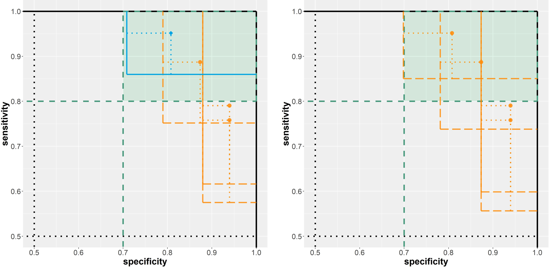
Exemplary analysis of synthetic example with four index tests. Region of interest (
We perform a simulation study to evaluate and compare the multiple comparison procedures described in this work. Our primary goal is a comparison with regard to FWER and statistical power. The (disjunctive) statistical power is the probability of obtaining at least one rejection of a false null hypothesis
Key features of simulation study.
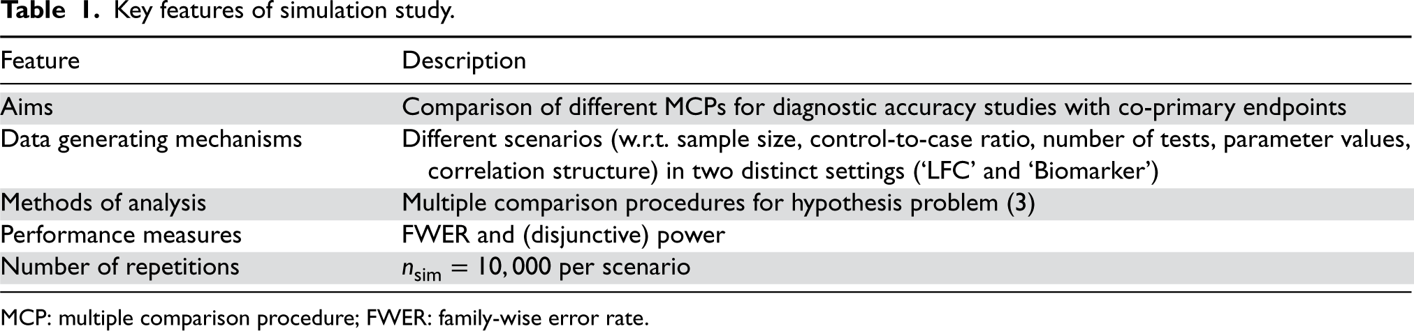
Key features of simulation study.
MCP: multiple comparison procedure; FWER: family-wise error rate.
For both simulation settings, many different scenarios are considered which are described by a number of design parameters (setting, sample size, control-to-case ratio, number of tests, parameter values, and correlation structure). For each scenario,
All numerical experiments presented in this work are reproducible by means of the new R package
As the source code for all statistical methods is available in the
In the first setting, a single synthetic data set consists of two separate samples for diseased and healthy. For that matter, two different multivariate Binomial models are employed to generate binary data matrices 
In this scenario, we focus on LFCs which are defined as parameters which maximize the FWER. As discussed in prior work,
6
an LFC in this case is defined by mean vectors 
The LFC setting discussed in the last section allows us to assess worst-case error rates. However, LFCs are rarely representative of real-world situations. 8 The goal of this second simulation study is thus to evaluate the multiple comparison procedures under more realistic parameter configurations.
To generate a single synthetic data set, we start by simulating 

These continuous scores 
Simulation study
LFC setting
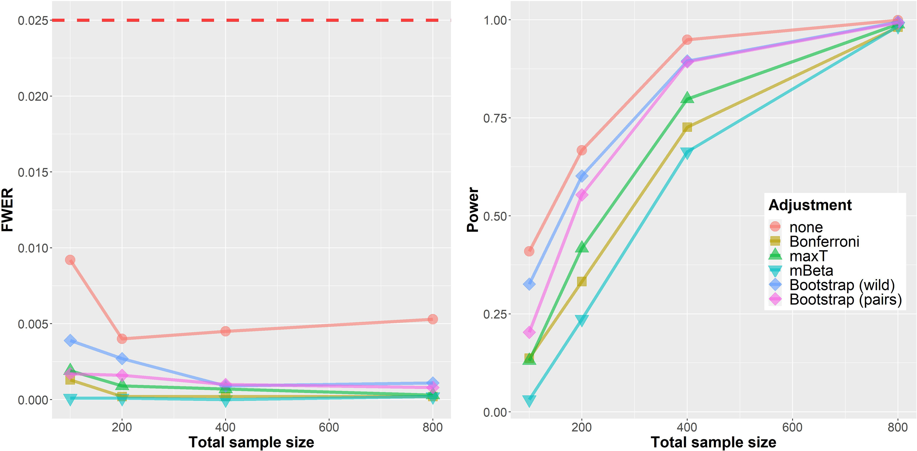
The simulation results from the LFC setting are displayed in Figure 2. On the left, the FWER is shown depending on the total sample size

Simulation results for the ‘LFC’ setting. Left: FWER. Right: Power. The horizontal axis shows the total sample size (cases and controls
First, applying no multiplicity adjustment at all clearly leads to a vastly increased FWER of
The right part of Figure 2 shows the (disjunctive) power for the same data instances after dropping the minimal acceptance criteria
Further analyses (simulation report
d
, section 2.1) indicate, that these findings for FWER and power remain qualitatively similar when only
In an additional experiment, the influence of different values of the prior parameter
Figure 3 shows results from the simulation in the more realistic biomarker setting. In contrast to the worst-case assessment in the last section, the FWER is below
Simulation results for the ‘Biomarker’ setting. Left: family-wise error rate (FWER). Right: Power. The horizontal axis shows the total sample size (cases and controls
Regarding statistical power the ordering of methods is mostly similar to the situation in the LFC setting. One important difference is the much better performance of both Bootstrap approaches which seem to adapt much better to the underlying generative distribution in this situation. Further results are shown in the separate simulation report (section 2.2). d
In a sensitivity analysis, the deviation from the bi-normal ROC model was investigated. For this matter, diagnostic markers were generated in a similar fashion but from a bi-exponential ROC model. This resulted in increased rejection rates for all procedures, most noticeably for the parametric approaches (no adjustment, Bonferroni and maxT). However, the FWER was still far below the nominal significance level in all simulation scenarios. Details are provided in the simulation report (section 2.3.1). d
To conclude, we apply our methodology to real-world data and interpret the results. For that matter, the pairs bootstrap approach is applied in the two motivating example scenarios introduced at the beginning of this work. To formalize our requirement that high sensitivity is prioritized, we define the minimal acceptance criteria as
Scenario A: Biomarker assessment
The most promising of the 15 investigated classification rules in terms of diagnostic accuracy on the evaluation data (212 cases and 357 controls) is the maximal area of any present cell nucleus with a threshold of
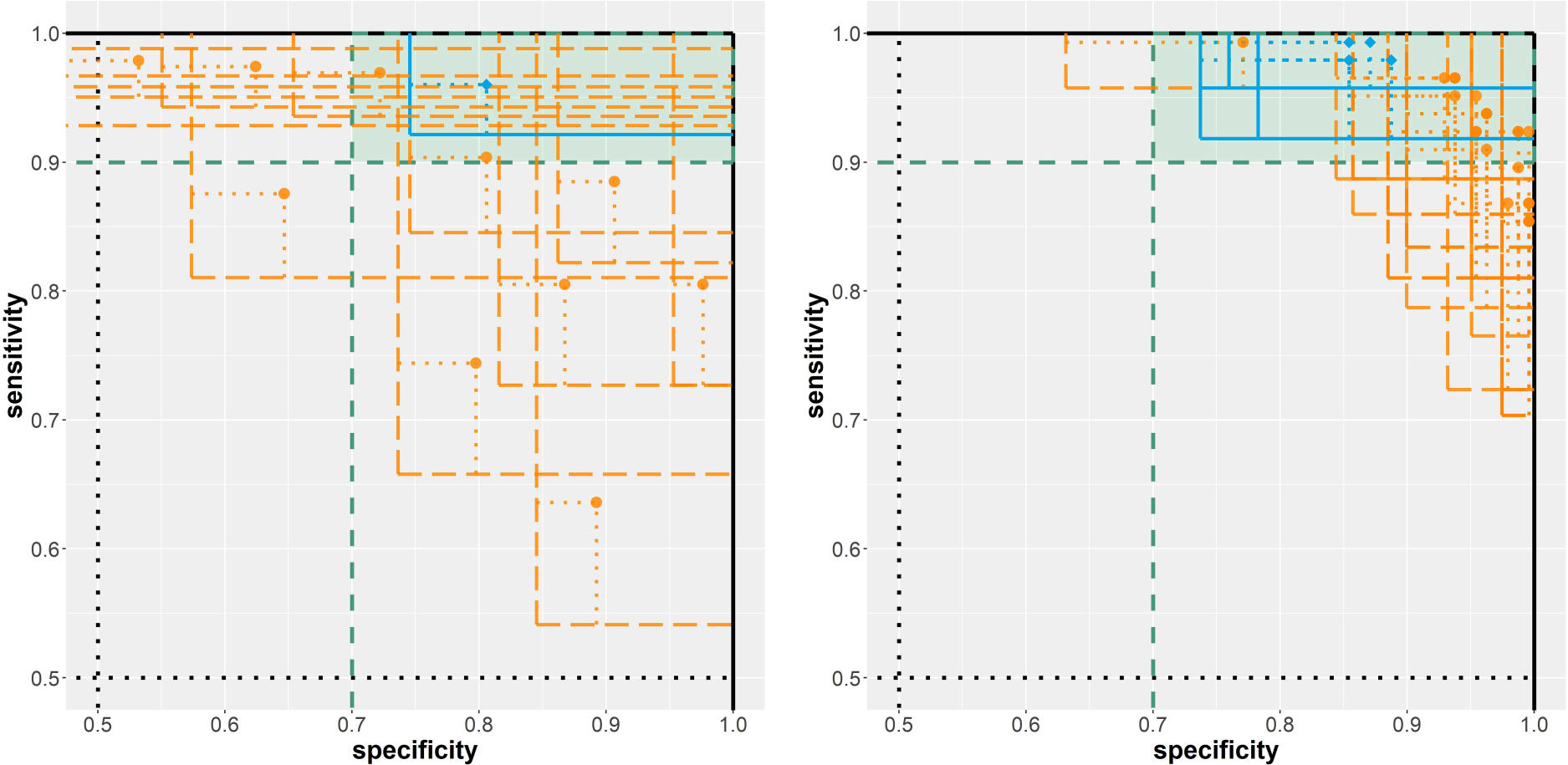
Results from the analysis of the two breast cancer diagnosis example scenarios. Left: biomarker assessment (scenario A). Right: risk model evaluation (scenario B). Solid/blue lines imply a rejected null hypothesis; dashed/orange lines imply a non-rejected null hypothesis.
In total, 25 risk prediction models were assessed on the evaluation data (71 cases, 119 controls). For four models, the null hypothesis
Discussion
In this work, we investigated statistical inference methods for diagnostic accuracy studies with multiple index tests and co-primary endpoints sensitivity and specificity. Multiplicity corrections are relevant in this context as omitting a suitable correction can otherwise induce overoptimistic results and inflated error rates. While a control is easily possible using a traditional (FWER) correction for all
We conducted an extensive simulation study to compare five multiple comparison procedures with regards to FWER and statistical power. All five procedures are capable of controlling the FWER at least asymptotically. The Bonferroni adjustment and maxT approaches both need quite large sample sizes to reach the target significance level. This, however, depends crucially on the control-to-cases ratio. A more skewed class distribution results in higher sample size demand. The Bayesian mBeta approach and the two Bootstrap (pairs and wild) procedures managed to control the FWER much better under LFCs. Based on the simulation study, we recommend the use of the pairs bootstrap approach. This approach yielded good FWER control for small sample sizes and competitive power in realistic scenarios. The wild bootstrap approach has a very similar performance, but the method is more complex, has more design choices, and was not originally designed to be used for binary data. For larger sample sizes, the maxT approach is a competitive alternative and easier to apply compared to the bootstrap procedures. The Bonferroni method is by far the easiest method to apply but too conservative in some situations and as such suboptimal.
In this work, we focused on the FWER and the statistical power. In our framework, point estimates are slightly shrunk due to the implemented minor regularization to avoid singular (co)variance estimates. However, point estimates were not adjusted for multiplicity. It has been demonstrated that the maxT approach can be utilized to obtain median-conservative point estimators.8,6 This generic approach could also be adapted to the other multiple comparison procedures.
All investigated methods can be adapted to the case that not only two (diseased and healthy) subpopulations need to be distinguished but more than two subpopulations, for example, different disease severities. This capability is already implemented in the
Footnotes
Declaration of conflicting interests
The authors declared no potential conflicts of interest with respect to the research, authorship, and/or publication of this article.
Funding
The authors received no financial support for the research, authorship, and/or publication of this article.