Evaluation of multiple prediction models: A novel view on model selection and performance assessment

Abstract

Model selection and performance assessment for prediction models are important tasks in machine learning, e.g. for the development of medical diagnosis or prognosis rules based on complex data. A common approach is to select the best model via cross-validation and to evaluate this final model on an independent dataset. In this work, we propose to instead evaluate several models simultaneously. These may result from varied hyperparameters or completely different learning algorithms. Our main goal is to increase the probability to correctly identify a model that performs sufficiently well. In this case, adjusting for multiplicity is necessary in the evaluation stage to avoid an inflation of the family wise error rate. We apply the so-called maxT-approach which is based on the joint distribution of test statistics and suitable to (approximately) control the family-wise error rate for a wide variety of performance measures. We conclude that evaluating only a single final model is suboptimal. Instead, several promising models should be evaluated simultaneously, e.g. all models within one standard error of the best validation model. This strategy has proven to increase the probability to correctly identify a good model as well as the final model performance in extensive simulation studies.

1 Introduction

Accurate and reliable diagnosis and prognosis are of utmost importance in clinical practice. New technologies rapidly add a vast variety of data sources that may be used as potential predictors. More often than not, these data are complex and high dimensional. As a result, many efforts are made to provide trustworthy diagnostic tools in the form of prediction models obtained via machine learning techniques.^1–4 A recent example is the application of deep learning for tumor classification based on imaging mass spectrometry data. ⁵ A major challenge in this process is the selection of a good model and a reliable assessment of its predictive performance. In this work, we address both questions with particular focus on increasing statistical power for model evaluation while avoiding overoptimistic claims regarding the final model performance.

In the following, we consider the problem of predicting a target variable Y (dependent variable) from a set of features $\mathbf{X}$ (independent variables). In supervised machine learning, this is achieved by learning a deterministic function $\hat{f}$ which provides a prediction $\hat{y}=\hat{f}(\mathbf{x})$ based on the observed features $\mathbf{x}$ . In practice, this is accomplished by a learning algorithm A which learns $\hat{f}$ from the training data $\mathcal{T}$ , that is to say $\hat{f}=A(\mathcal{T})$ . We assume that the $n_{\mathcal{T}}$ observations are sampled i.i.d. from the unknown joint probability distribution $\mathfrak{D}={\mathfrak{D}}_{(\mathbf{X}\mathbf{,}\mathbf{Y})}$ from $\mathbf{X}$ and Y or $\mathcal{T}\sim {\mathfrak{D}}^{n_{\mathcal{T}}}$ for short. A typical example is medical diagnosis, e.g. prediction if a patient has a certain disease (Y = 1) or not (Y = 0) based on a collection of clinical measurements $\mathbf{X}\mathbf{\in }ℝ\mathbf{P}$ , where $P\in \mathbb{N}$ denotes the number of features. In contrast to this (binary) classification task, the case of $Y\in ℝ$ is referred to as a regression problem. We refer to standard references for a throughout introduction to fundamental machine learning concepts.^6,7

Once a prediction model $\hat{f}$ has been learned from $\mathcal{T}$ , we consider it as a given, deterministic function. An important task is then the evaluation of its predictive performance. The (generalization) performance of $\hat{f}$ is defined as $\vartheta ={\vartheta }_s(\hat{f})=\mathbb{E}\mathfrak{D}[s(\hat{f}(\mathbf{X})\mathbf{,}\mathbf{Y})]$ , where $s(\hat{y},y)$ is a deterministic, real-valued function which measures the similarity of prediction $\hat{y}=\hat{f}(\mathbf{x})$ and truth y. In some cases, one rather defines a dissimilarity measure (loss) $d(\hat{y},y)$ and accordingly the (generalization) error ${\vartheta }_d(\hat{f})$ . Typical examples for a similarity and dissimilarity measure are $s(\hat{y},y)=11(\hat{y}=y)$ , defining classification accuracy, and $d(\hat{y},y)=(\hat{y}-y)2$ , defining the mean squared error (MSE) for a regression problem. In the following, we only refer to ϑ as performance. The question on how to choose s for a specific application is not covered in this work and we refer to the existing literature for a comparison of different (dis)similarity measures.^8–12

A natural estimator for ϑ is the empirical performance $\hat{\vartheta }=\hat{\vartheta }(\hat{f},\mathcal{D})=\frac{1}{n_{\mathcal{D}}}\sum _{i=1}^{n_{\mathcal{D}}}s(\hat{f}(\hspace{0.17em}\mathbf{x}\mathbf{i}),y_i)$ on a dataset $\mathcal{D}\sim {\mathfrak{D}}^{n_{\mathcal{D}}}$ . It is well known that estimation of ϑ on the training data $\mathcal{T}$ may lead to overly optimistic (upward biased) performance estimates, if the learning algorithm overfits the training data. The usual recommendation is therefore to estimate ϑ on validation data $\mathcal{V}\sim {\mathfrak{D}}^{n_v}$ that is independent of $\mathcal{T}$ .

In practice, usually not only a single but rather multiple learning algorithms A _m , $m\in \mathcal{M}=\{1,\dots ,M\}$ , are considered. The algorithms A _m may be completely different, e.g. a logistic regression versus a tree-based model, or just differ regarding the choice of a hyperparameter like the strength of a penalty term. Two important aspects of machine learning are how to select a model $f_{m^{*}}$ and estimate its performance ${\vartheta }_{m^{*}}$ . The naive approach of estimating ${\vartheta }_m=\vartheta ({\hat{f}}_m)$ for all models, on the same dataset $\mathcal{V}$ and then choosing the empirically best model $m^{*}=\text{argma}{\text{x}}_{m\in \mathcal{M}}{\hat{\vartheta }}_m(\mathcal{V})$ has the severe downside that the estimate ${\hat{\vartheta }}_{m^{*}}(\mathcal{V})$ for ${\vartheta }_{m^{*}}$ is usually biased upward. This is often referred to as selection-induced bias which is particularly important in case statistical inference regarding the unknown parameter ${\vartheta }_{m^{*}}$ is the ultimate goal, e.g. deciding if ${\vartheta }_{m^{*}}>{\vartheta }_0$ for a performance threshold ${\vartheta }_0$ . Statistical inference for model performance in form of test decisions or interval estimates may not always be needed in machine learning applications, but it certainly is in regulated environments like evaluation of diagnostic or prognostic devices and procedures in medical research.^13,14

The predominant recommendation in the literature concerning model selection and evaluation is to sample learning data $\mathcal{L}\sim {\mathfrak{D}}^{n_{\mathcal{L}}}$ and evaluation data $\mathcal{E}\sim {\mathfrak{D}}^{n_{\mathcal{E}}}$ and perform the following steps^6,8,15–17

Learning: The learning data $\mathcal{L}$ is split into training set $\mathcal{T}$ and validation set $\mathcal{V}$ . The random splitting $\mathcal{L}=\mathcal{T}{\cup }_{\stackrel{·}{\hspace{0.17em}}}\mathcal{V}$ may be repeated multiple times leading to techniques like (repeated) K-fold-cross-validation and different bootstrap versions, cf. ¹⁸ and references therein. In this case, the resulting estimates $\hat{\vartheta }(A_m(\mathcal{T}),\mathcal{V})$ are averaged to estimate the expected performance of each algorithms A _m . The algorithm $m^{*}$ which yields the highest estimated (expected) performance is selected and used to learn the final model ${\hat{f}}_{m^{*}}=A_{m^{*}}(\mathcal{L})$ on the whole learning data $\mathcal{L}$ .

Evaluation: The performance of the final model ${\hat{f}}_{m^{*}}=A_{m^{*}}(\mathcal{L})$ is assessed on the independent evaluation set $\mathcal{E}$ . It is frequently emphasized that only a single model shall be evaluated on $\mathcal{E}$ to enable an unbiased performance estimation. A statistical test $\varphi ⋮\mathcal{E}\to \{0,1\}$ may be used to decide if the null hypothesis $H_0⋮{\vartheta }_{m^{*}}\le {\vartheta }_0$ can be rejected in favor of alternative $H_1⋮{\vartheta }_{m^{*}}>{\vartheta }_0$ .

In the machine learning literature, $\mathcal{E}$ is commonly referred to as the test set. Unfortunately, $\mathcal{E}$ is also sometimes referred to as validation data. To avoid confusion, we will only use the term evaluation data for $\mathcal{E}$ and validation data for $\mathcal{V}\subset \mathcal{L}$ in the following.

The default learning-evaluation-strategy described above has several advantages. Mainly, it limits the danger of overfitting to the training data and it allows to obtain an unbiased estimate of ${\vartheta }_{m^{*}}$ , the performance of the final model ${\hat{f}}_{m^{*}}$ . Furthermore, it is usually not difficult to derive a statistical test for the (one-sided) null hypothesis $H_0^{m^{*}}⋮{\vartheta }_{m^{*}}\le {\vartheta }_0$ . The threshold ${\vartheta }_0$ needs to be defined prior to the evaluation study and should reflect the minimal required performance for the application at hand. For diagnostic devices in medical applications, $1-{\vartheta }_0$ expresses the sacrifice in accuracy one is willing to make compared to the reference standard due to other advantages of the new procedure (e.g. lower invasiveness or costs). It is also possible to estimate ${\vartheta }_0=\vartheta ({\hat{f}}_0)$ of an established comparator ${\hat{f}}_0$ on the same evaluation data for a direct comparison. For simplicity, we will however assume that ${\vartheta }_0$ is known in the remainder of the work. Requiring that the null hypothesis $H_0^{m^{*}}⋮{\vartheta }_{m^{*}}\le {\vartheta }_0$ needs to be rejected before implementing a new diagnostic tool in clinical practice expresses that we would rather err on the side of caution. That is to say, we would rather not implement a good model (type 2 error) than falsely implementing a bad model (type 1 error). This is in particular true in critical applications where life threatening decisions may be based on the diagnostic results. This approach is established in particular in phase 4 or phase 3 diagnostic accuracy studies, depending on the taxonomy.^9,19 Furthermore, several works highlight that (external) evaluation studies for the final model are important but rarely conducted in practice.^13,14,20,21

However, it might also be disadvantageous to select only one model for final evaluation, namely if the selected model $m^{*}$ is far worse than one of its competitors $m\in \mathcal{M}$ . This is a relevant threat in practice when validation performance estimates are highly variable, e.g. in case of few validation observations. Another obstacle might be non-representative learning samples, i.e. when the data used for model development strongly deviates from the target population in key characteristics. In our experience, this is not unlikely in medical research when the learning data is collected retrospectively from a wide variety of data sources. For instance, the learning data might differ strongly from the target population regarding relevant features like age, sex or comorbidities. The prospective evaluation study, however, is conducted in a cohort fulfilling rigorous inclusion criteria leading to charasteristics closer to the target population. Performance estimates during learning and evaluation phase might hence differ substantially. A similar effect might originate from ongoing advances of sample preparation procedures and biomarker assays over time, i.e. from $\mathcal{L}$ (past) to $\mathcal{E}$ (future). Such developments are certainly positive in general, but may nonetheless lower the chances to correctly identify a truly good model with regards to samples from the target distribution $\mathfrak{D}$ based on the non-representative learning data.

As a result, we may thus be in danger to conduct correct inference for an underperforming model. A potential remedy is to evaluate multiple models ${\mathcal{M}}^{*}\subset \mathcal{M}$ on the evaluation data with the goal to increase the probability to correctly identify at least one model $m^{*}\in {\mathcal{M}}^{*}$ which is able to outperform the benchmark ${\vartheta }_0$ . This problem can be stated as a multiple test problem specified by the following system of null hypotheses

$${\mathcal{H}}^{*}=\{H_0^{m^{*}}⋮{\vartheta }_{m^{*}}\le {\vartheta }_0,m^{*}\in {\mathcal{M}}^{*}\}$$

(1)

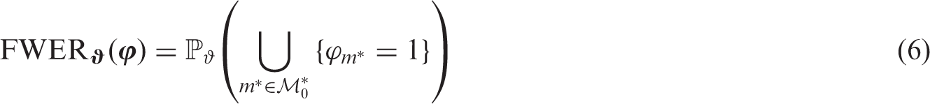
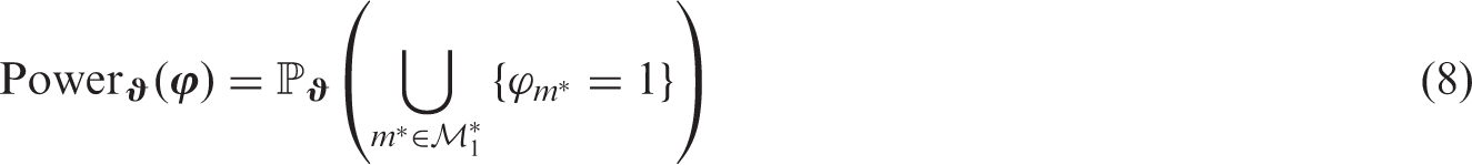
Inference regarding ${\mathcal{H}}^{*}$ may be conducted via a multiple test, i.e. a mapping $\mathbf{\varphi }⋮\mathcal{E}\to \{0,1\}{M}^{*}$ whereby ${\varphi }_{m^{*}}=1$ implies that hypothesis $H_0^{m^{*}}$ is rejected. $\mathbf{\varphi }$ is expected to control the family wise error rate (FWER), a generalization of the type 1 error for multiple hypothesis tests. In addition, we consider the disjunctive power as an important characteristic of $\mathbf{\varphi }$ , which is defined as the probability to correctly reject at least one false null hypothesis. When rejecting a single null hypothesis from ${\mathcal{H}}^{*}$ , we also reject the global null hypothesis

$$G^{*}=\bigcap _{m^{*}\in {\mathcal{M}}^{*}}{H}_0^{m^{*}}$$

(2)

Multiple hypothesis testing is not commonly employed in model evaluation practice although different approaches have been showcased and compared in this context. ²² This might stem from the fact that the omnipresent recommendation to completely seperate model selection and evaluation results in a valid and easy-to-use strategy to avoid an overoptimistic performance assessment. To avoid the beforementioned downsides associated with this strategy when the uncertainty regarding model selection is high, we will investigate a particular multiple test in this work. The so-called maxT-approach is based on the joint distribution of the test statistics and assumes (approximate) normality. Technical details are provided in the next section. We note that, even if the validation ranking is correct, we might benefit from evaluating multiple models in terms of statistical power.

In this context it should also be noted that in the usual framework, the properties of the multiple test $\mathbf{\varphi }$ for ${\mathcal{H}}^{*}$ , i.e. FWER control and maximization of power, are assessed conditional on the previously conducted model selection. Formally, we assume that this selection is based on a selection rule which is a mapping $\mathbf{r}\mathbf{:}\mathcal{L}\mathbf{\to }{\mathcal{M}}^{\mathbf{*}}\mathbf{\subset }\mathcal{M}$ . That is to say, a subset of models ${\mathcal{M}}^{*}$ is selected for evaluation based on the learning data, in particular the validation estimates $({\hat{\vartheta }}_m(\mathcal{V}))m\in \mathcal{M}$ . In order to link model selection and performance assessment, we propose to extend a given selection rule $\mathbf{r}$ and a multiple test $\mathbf{\varphi }$ for ${\mathcal{H}}^{*}$ to a multiple test $\mathbf{\psi }=({\psi }_m)m\in \mathcal{M}$ for the initial hypothesis system

$$\mathcal{H}=\{H_0^m⋮{\vartheta }_m\le {\vartheta }_0,m\in \mathcal{M}\}$$

(3)

by setting

$${\psi }_m(\mathcal{E})=\begin{array}{c}\{\begin{array}{cc}0& \hfill \text{ifm}\notin {\mathcal{M}}^{*},\hfill \\ {\varphi }_m(\mathcal{E})& \hfill \text{ifm}\in {\mathcal{M}}^{*}\hfill \end{array}\end{array}$$

(4)

This means that we evaluate all models $m\notin {\mathcal{M}}^{*}$ negatively, i.e. do not reject the according null hypothesis. With definition (4) we formalize what is implicitly done in practice, namely to ‘spend’ all of the significance level α on the evaluation of the selected model(s) and neglect all other models. We perceive the global null

$$G=\bigcap _{m\in \mathcal{M}}{H}_0^m$$

(5)

associated with $\mathcal{H}$ as much more relevant in practice than $G^{*}$ associated to ${\mathcal{H}}^{*}$ . That is, it is more natural to ask if any of the candidate models considered in the first place ( $m\in \mathcal{M}$ ) outperforms the performance benchmark ${\vartheta }_0$ rather than asking the same question restricted to the few (or single) models $m^{*}\in {\mathcal{M}}^{*}$ which were chosen to be evaluated. This approach enables us to assess the quality of model selection and evaluation together.

Our main research questions can be stated as follows: (1) In which situations is it beneficial to evaluate more than one model? (2) How do different model selection rules perform relative to each other regarding FWER control, statistical power and estimation bias? The remainder of this work is structured as follows: In the second section, a few important concepts from multiple testing theory are defined. In addition, we show that our approach is applicable for a wide variety of performance measures, namely if the empirical performance estimate (sample average) is used. In the third section, we will present the results from numerical experiments we conducted to compare several heuristic model selection rules in conjunction with the maxT-approach with regards to FWER, power and estimation bias. In the fourth section, our evaluation strategy is applied to two real datasets. Finally, in the last section, we will discuss our findings and propose possible extensions to our work.

2 Statistical model and theoretical aspects

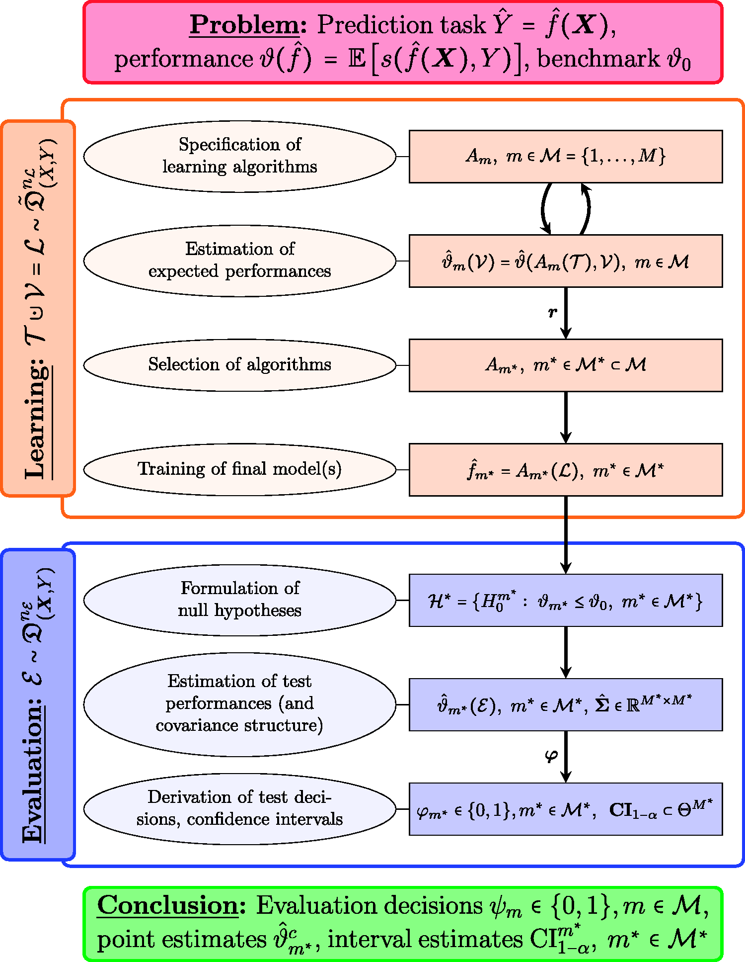
We will assume the following scenario: Given a prediction task $\hat{Y}=\hat{f}(\mathbf{X})$ , a similarity measure s and learning data $\mathcal{L}$ , the goal is to provide empirical evidence that at least one of the candidate models ${\hat{f}}_m=A_m(\mathcal{L}),m\in \mathcal{M}$ , can outperform the benchmark ${\vartheta }_0$ . The evaluation is conducted via a selection rule $\mathbf{r}$ , an evaluation sample $\mathcal{E}\sim {\mathfrak{D}}^{n_{\mathcal{E}}}$ and a multiple test $\mathbf{\varphi }$ . We are interested in properties of the multiple test $\mathbf{\psi }=(\mathbf{r}\mathbf{,}\mathbf{\varphi })$ introduced via equation (4) in terms FWER and power and the bias of the performance estimate(s). As the traditional assumption $\mathcal{L}\sim {\mathfrak{D}}^{n_{\mathcal{L}}}$ may be violated in practice, we will also consider the case were $\mathcal{L}\sim {\stackrel{\sim }{\mathfrak{D}}}^{n_{\mathcal{L}}}$ is sampled from an altered distribution $\stackrel{\sim }{\mathfrak{D}}$ . Our perception of the learning-evaluation process is depicted in Figure 1, whereby some aspects will be derived in the following. Note that the learning phase may be iterative which is indicated by the double arrow between training and validation. In contrast, the hypotheses and hence the prediction models in the evaluation phase cannot be changed after the data has been observed when the goal is strict control of the type 1 error.

Figure 1.

Schematic representation of the machine learning and evaluation process.

2.1 Multiple testing in model evaluation

In the following we introduce some important definitions, mainly adopted from Dickhaus. ²³ The system of null hypothesis ${\mathcal{H}}^{*}$ is defined in equation (1). A (non-randomized) multiple test for ${\mathcal{H}}^{*}$ is a mapping $\mathbf{\varphi }⋮\mathcal{E}\to \{0,1\}{M}^{*}$ . For $m^{*}\in {\mathcal{M}}^{*}$ the null hypothesis $H_0^{m^{*}}$ gets rejected if ${\varphi }_{m^{*}}=1$ . The family-wise error rate of $\mathbf{\varphi }$ is defined as

$$\text{FWE}\text{R}\vartheta (\mathbf{\varphi })=\mathbb{P}\vartheta (\bigcup _{m^{*}\in {\mathcal{M}}_0^{*}}\{{\varphi }_{m^{*}}=1\})$$

(6)

where ${\mathcal{M}}_0^{*}\subset {\mathcal{M}}^{*}$ is defined as the set of indexes $m^{*}$ such that $H_0^{m^{*}}$ is true which depends on the true parameter vector ϑ. This probability to make any false positive claim shall be bounded by the significance level $\alpha \in (0,1)$ . Formally, ϕ is said to control the FWER strongly if

$$\forall \mathbf{\vartheta }\mathbf{\in }\mathbf{\Theta }\mathbf{:}\text{FWE}\text{R}\mathbf{\vartheta }(\mathbf{\varphi })\mathbf{\le }\mathbf{\alpha }$$

(7)

whereby $\mathbf{\Theta }$ is the parameter space. This is a very important property, as without FWER control or another way of limiting false positive test decision any multiple test is essentially pointless. Regarding type 2 errors (false negative test decisions), the disjunctive (or 1-minimal) power is defined as

$$\text{Powe}\text{r}\vartheta (\mathbf{\varphi })=\mathbb{P}\vartheta (\bigcup _{m^{*}\in {\mathcal{M}}_1^{*}}\{{\varphi }_{m^{*}}=1\})$$

(8)

whereby ${\mathcal{M}}_1^{*}={\mathcal{M}}^{*}\setminus {\mathcal{M}}_0^{*}$ . A usual way to choose between different multiple tests for the same problem is to seek maximum power given control of the FWER at a specific significance level, e.g. $\alpha =0.05$ . There are other power concepts in multiple testing, aiming at the simultaneous rejection of several false hypotheses, which are not considered in this work. ²⁴

2.2 The maxT-approach

We will consider one particular multiple test for ${\mathcal{H}}^{*}$ in this work, namely the so-called maxT-approach which is also called projection method in the literature.^23,25

Let $\hat{\vartheta }=({\hat{\vartheta }}_{m^{*}})m^{*}\in {\mathcal{M}}^{*}$ be the vector of estimates for the unknown parameter $\mathbf{\vartheta }\mathbf{=}(\hspace{0.17em}\mathbf{\vartheta }{\mathbf{m}}^{\mathbf{*}}){\mathbf{m}}^{\mathbf{*}}\mathbf{\in }{\mathcal{M}}^{\mathbf{*}}$ . By $n=n_{\mathcal{E}}$ we denote the evaluation set size. Let furthermore $\hat{\mathbf{\Sigma }}={\hat{\mathbf{\Sigma }}}_n$ be an estimate of the covariance matrix $\mathbf{\Sigma }=\text{cov}(\hat{\vartheta })$ with $a_n{\hat{\mathbf{\Sigma }}}_n\to \mathbb{P}\mathbf{\Sigma }$ where a _n is a nondecreasing sequence. In addition, we assume that $\hat{\vartheta }=\widehat{{\vartheta }_n}$ follows asymptotically a multivariate normal distribution, i.e. $a_n^{1/2}(\widehat{{\vartheta }_n}-\mathbf{\vartheta })\mathbf{\to }\mathcal{D}{\mathcal{N}}_{{\mathbf{M}}^{\mathbf{*}}}(0\mathbf{,}\mathbf{\Sigma })$ . We condense these two assumptions to

$$\hat{\vartheta }\stackrel{·}{\sim }{\mathcal{N}}_{M^{*}}(\mathbf{\vartheta }\mathbf{,}\hat{\mathbf{\Sigma }})$$

(9)

to describe the approximate distribution of $\hat{\vartheta }$ . We define the test statistics $T_{m^{*}}=({\hat{\vartheta }}_{m^{*}}-{\vartheta }_0)/\widehat{\text{se}}({\hat{\vartheta }}_{m^{*}})$ or $\mathbf{T}\mathbf{=}\widehat{{\mathbf{D}}^{\mathbf{-}1\mathbf{/}2}}(\hat{\mathbf{\vartheta }}\mathbf{-}\hspace{0.17em}\mathbf{\vartheta }0)$ in vectorized form, whereby $\hat{D}=\text{diag}(\hat{\Sigma })$ . Assumption (9) entails

$$\mathbf{\vartheta }\mathbf{=}\hspace{0.17em}\mathbf{\vartheta }0\mathbf{\hspace{1em}\hspace{1em}\hspace{1em}}\mathbf{\Rightarrow }\mathbf{\hspace{1em}\hspace{1em}\hspace{1em}}\mathbf{T}\stackrel{·}{\mathbf{\sim }}{\mathcal{N}}_{{\mathbf{M}}^{\mathbf{*}}}(0\mathbf{,}\hat{\mathbf{R}})$$

(10)

where $\hat{R}=\widehat{D^{-1/2}}\hat{\Sigma }\widehat{D^{-1/2}}$ is the estimated correlation matrix of $\hat{\vartheta }$ . From this, the approximate distribution of the maximum test statistic can be derived as

$$\mathbb{P}({max}_{m^{*}}(T_{m^{*}})\le t)\approx {\Phi }_{M^{*}}(\mathbf{t}\mathbf{,}\hat{\mathbf{R}})\mathbf{=}{\mathbf{\int }}_{\mathbf{-}\mathbf{\infty }}^{\mathbf{t}}\mathbf{\dots }{\mathbf{\int }}_{\mathbf{-}\mathbf{\infty }}^{\mathbf{t}}\hspace{0.17em}\mathbf{\phi }{\mathbf{M}}^{\mathbf{*}}(\mathbf{x}\mathbf{,}\hat{\mathbf{R}})\text{d}1\mathbf{x}$$

(11)

where ${\phi }_{M^{*}}(·,\hat{R})$ is the density function of the $M^{*}$ -dimensional multivariate normal distribution with mean $0$ and covariance matrix $\hat{R}$ . From this we can calculate the simultaneous critical value $c_{\alpha }\in ℝ$ by solving ${\Phi }_{M^{*}}(\hspace{0.17em}\mathbf{c}\mathbf{\alpha },\hat{R})=1-\alpha$ numerically for $\hspace{0.17em}\mathbf{c}\mathbf{\alpha }=(c_{\alpha },\dots ,c_{\alpha })$ . This defines a multiple test for ${\mathcal{H}}^{*}$ by rejecting $H_{m^{*}}$ if and only if $t_{m^{*}}>c_{\alpha }$ . Calibrating $c_{\alpha }$ under the global null $G^{*}$ yields weak control of the FWER. In this case, even strong FWER-control is warranted because the subset pivotality condition (SPC) is met. ²³ (p.48). One might also construct approximate simultaneous (e.g. lower) confidence intervals with confidence level $1-\alpha$ via

$$\mathbf{C}\hspace{0.17em}\mathbf{I}1-\alpha ={\times }_{{\text{m}}^{*}\in {\text{M}}^{*}}[{\hat{\vartheta }}_{{\text{m}}^{*}}-{\text{c}}_{\alpha }·\widehat{\text{se}}({\hat{\vartheta }}_{{\text{m}}^{*}}),\infty )$$

(12)

The maxT-approach is a simultaneous test procedure (STP), meaning that all test statistics are compared to the same critical value. Taking into account the correlation between the performance estimates results in an increased rejection rate compared to simpler procedures when the correlations are positive. For instance, the critical value $c_{\alpha }$ is less than or equal to $\Phi ((1-\alpha )1/M^{*})$ which corresponds to a Šidák correction with equality in case the test statistics are uncorrelated ²³ (p.55).

One might ask the question, in which situations it is more efficient to test multiple hypothesis instead of just one. By efficiency we refer to distjunctive power as defined in equation (8). If ϑ and $\mathbf{\Sigma }=\hspace{0.17em}\mathbf{\Sigma }n={\mathbf{D}}_{\mathbf{n}}^{1\mathbf{/}2}{\mathbf{RD}}_{\mathbf{n}}^{1\mathbf{/}2}$ are assumed to be known, $\text{Power}\vartheta$ can be calculated explicitly. For $\mathbf{\vartheta }\mathbf{\in }\mathbf{\Theta }\mathbf{\setminus }{\mathbf{G}}^{\mathbf{*}}$ the power is given as one minus the probability that all observed test statistics are smaller than $c_{\alpha }$ , i.e.

$$\text{Powe}\text{r}\vartheta (\hspace{0.17em}\mathbf{\varphi }\max T)=1-{\Phi }_{M^{*}}(\hspace{0.17em}\mathbf{c}\mathbf{\alpha }-{\mathbf{D}}_{\mathbf{n}}^{\mathbf{-}1\mathbf{/}2}(\mathbf{\vartheta }\mathbf{-}\hspace{0.17em}\mathbf{\vartheta }0)\mathbf{,}\mathbf{R})$$

(13)

In case not all null hypotheses are false, the quantities $\mathbf{\vartheta }\mathbf{,}\hspace{0.17em}\mathbf{D}\mathbf{n}$ and $\mathbf{R}$ in equation (13) need to be restricted to the index set of false null hypothesis. This may be used for an approximation of $\text{Powe}{\text{r}}_{\vartheta }$ when assuming certain $\mathbf{\vartheta }\mathbf{,}\hspace{0.17em}\mathbf{\Sigma }\mathbf{n}$ and evaluation sample size $n=n_{\mathcal{E}}$ . Conversely, the sample size n to achieve a specific power may also be calculated. However, since equation (13) ignores the fact that $\mathbf{\Sigma }$ needs to be estimated, simulations may yield a more precise power estimate.

2.3 Performance estimation

We will now restrict our attention to binary classification, i.e. $Y\in \{0,1\}$ , as this case is most important for medical diagnosis and consider overall accuracy as the performance measure defined through $\vartheta =\mathbb{E}\mathfrak{D}[11(\hat{f}(\mathbf{X})\mathbf{=}\mathbf{Y})]\mathbf{=}\mathbb{P}(\hat{\mathbf{f}}(\mathbf{X})\mathbf{=}\mathbf{Y})$ . From the observed evaluation data $\mathcal{E}=\{(\hspace{0.17em}\mathbf{x}\mathbf{i},y_i)\}i=1,\dots ,n$ the actual relevant similarity matrix

$$\mathbf{S}\mathbf{=}\mathbf{(}11({\hat{\mathbf{f}}}_{{\mathbf{m}}^{\mathbf{*}}}(\hspace{0.17em}\mathbf{x}\mathbf{i})\mathbf{=}\hspace{0.17em}\mathbf{y}\mathbf{i}){\mathbf{)}}_{\genfrac{}{}{0ex}{}{\mathbf{i}\mathbf{=}1\mathbf{,}\mathbf{\dots }\mathbf{,}\mathbf{n}}{{\mathbf{m}}^{\mathbf{*}}\mathbf{\in }{\mathcal{M}}^{\mathbf{*}}}}$$

(14)

is derived by applying all selected models ${\hat{f}}_{m^{*}}$ to the observed feature data $\hspace{0.17em}\mathbf{x}\mathbf{i}$ . Note that this step is deterministic, given that all prediction rules ${\hat{f}}_{m^{*}}$ are deterministic.

The true performances ${\vartheta }_{m^{*}}$ can be estimated as the sample proportions of correct predictions ${\hat{\vartheta }}_{m^{*}}=\frac{1}{n}\sum _{i=1}^{n}11({\hat{f}}_{m^{*}}(\hspace{0.17em}\mathbf{x}\mathbf{i})=y_i)$ , the column means of $\mathbf{S}$ . A consistent estimate for the covariance matrix $\mathbf{\Sigma }$ of ϑ is given by $\hat{\mathbf{\Sigma }}={\hat{\mathbf{\Sigma }}}_n$ , the sample covariance matrix of $\mathbf{S}$ (divided by n). The entries of $\hat{\mathbf{\Sigma }}$ can be written as

$${\hat{\sigma }}_{m^{*}{k}^{*}}=\frac{{\hat{\pi }}_{m^{*}{k}^{*}}-{\hat{\vartheta }}_{m^{*}}{\hat{\vartheta }}_{k^{*}}}{n}$$

(15)

where ${\hat{\pi }}_{m^{*}{k}^{*}}=\frac{1}{n}\sum _{i=1}^{n}11({\hat{f}}_{m^{*}}(\hspace{0.17em}\mathbf{x}\mathbf{i})={\hat{f}}_{k^{*}}(\hspace{0.17em}\mathbf{x}\mathbf{i})=y_i)$ is the estimated proportion of common correct predictions of model $m^{*}$ and $k^{*}$ . Due to the multivariate central limit theorem, ²⁶ the joint distribution of $\hat{\vartheta }$ is asymptotically multivariate normal

$$n^{1/2}(\widehat{{\vartheta }_n}-\mathbf{\vartheta })\mathbf{\to }\mathfrak{D}{\mathcal{N}}_{{\mathbf{M}}^{\mathbf{*}}}(0\mathbf{,}\mathbf{\Sigma })\mathbf{,}\mathbf{n}\mathbf{\to }\mathbf{\infty }$$

(16)

This result can be generalized to arbitrary similarity functions s as long as the estimator $\hat{\vartheta }=\frac{1}{n}\sum _{i=1}^{n}s(\hat{f}(x_i),y_i)$ is employed. This justifies assumption (9) and hence the use of the maxT-approach when the empirical performance estimator is used.

2.4 Model selection based on the evaluation data

Since we are no longer limited to evaluate only one model on $\mathcal{E}$ , the final model selection now needs to be conducted based on the evaluation data. When using the maxT-approach, the most obvious choice is $m^{**}=\text{argma}{\text{x}}_{m^{*}\in {\mathcal{M}}^{*}}{T}_{m^{*}}$ . For classification accuracy, this is equivalent to choosing $m^{**}=\text{argma}{\text{x}}_{m^{*}}{\hat{\vartheta }}_{m^{*}}$ because $\hat{\vartheta }\to t=(\hat{\vartheta }-{\vartheta }_0)/\sqrt{\hat{\vartheta }(1-\hat{\vartheta })/n}$ is a strictly increasing function. Of course, (non-)rejection of $H_0^{m^{**}}$ is equivalent to (non-)rejection of the global null hypothesis $G^{*}$ .

We expect that conducting the final model selection based on the evaluation data will again introduce an upward bias of the estimate ${\hat{\vartheta }}_{m^{**}}$ . One elegant way to correct for this bias is to calculate the lower bound of a one-sided simultaneous 50% confidence interval as an estimator for ${\vartheta }_{m^{**}}$ . More explicitly, for every selected model we define a corrected point estimate for ${\vartheta }_{m^{*}}$ as

$${\hat{\vartheta }}_{m^{*}}^c={\hat{\vartheta }}_{m^{*}}-c_{0.5}\widehat{\text{se}}({\hat{\vartheta }}_{m^{*}}),m^{*}\in {\mathcal{M}}^{*}$$

(17)

where $c_{0.5}$ satisfies ${\Phi }_{M^{*}}(\hspace{0.17em}\mathbf{c}0\mathbf{.}5,\hat{R})=0.5$ . Under the assumption of normality and a known covariance matrix we have

$$\mathbb{P}({\hat{\vartheta }}_{m^{**}}^c>{\vartheta }_{m^{**}})\le \mathbb{P}(\exists m^{*}\in {\mathcal{M}}^{*}⋮{\hat{\vartheta }}_{m^{*}}^c>{\vartheta }_{m^{*}})=0.5$$

(18)

as the event $E_1=\{{\hat{\vartheta }}_{m^{**}}^c>{\vartheta }_{m^{**}}\}$ implies $E_2=\{\exists m^{*}\in {\mathcal{M}}^{*}⋮{\hat{\vartheta }}_{m^{*}}^c>{\vartheta }_{m^{*}}\}$ . The estimator ${\hat{\vartheta }}_{m^{**}}^c$ is therefore (approximately) median-conservative. Equality in equation (18), which corresponds to median-unbiasedness of ${\hat{\vartheta }}_{m^{**}}^c$ , follows in the case when all selected models have the same true performance as in this case E₁ = E₂.

2.5 Transition from ${\mathcal{H}}^{*}$ to $\mathcal{H}$

As stated before, in the context of model selection and evaluation we perceive the hypothesis system $\mathcal{H}=\{H_0^m⋮{\vartheta }_m\le {\vartheta }_0,m\in \mathcal{M}\}$ as much more relevant than ${\mathcal{H}}^{*}=\{H_0^{m^{*}}⋮{\vartheta }_{m^{*}}\le {\vartheta }_0,m^{*}\in {\mathcal{M}}^{*}\}$ . We thus define a multiple test $\mathbf{\psi }$ for $\mathcal{H}$ by combining a selection rule $\mathbf{r}\mathbf{:}\mathcal{L}\mathbf{\to }{\mathcal{M}}^{\mathbf{*}}\mathbf{\subset }\mathcal{M}$ with a multiple test $\mathbf{\varphi }$ for ${\mathcal{H}}^{*}$ to a multiple test $\mathbf{\psi }=(\mathbf{r}\mathbf{,}\mathbf{\varphi })$ for $\mathcal{H}$ as given in equation (4). Due to this construction, $\mathbf{\psi }$ controls the FWER strongly for $\mathcal{H}$ if $\mathbf{\varphi }$ strongly controls the FWER for ${\mathcal{H}}^{*}$ for all ${\mathcal{M}}^{*}\subset \mathcal{M}$ . This is given (approximately) in our framework as pointed out in the statistical model section.

In summary, in the presented framework, we obtain corrected point estimates (17), a simultaneous confidence region (12) and test decisions ${\psi }_{m^{*}}={\varphi }_{m^{*}},m^{*}\in {\mathcal{M}}^{*}$ , for the selected models after having conducted the evaluation phase. Additionally, for all models $m\in \mathcal{M}\setminus {\mathcal{M}}^{*}$ which have not been selected we conclude ${\psi }_m=0$ , i.e. not to reject the null hypothesis $H_0^m$ , compare Figure 1.

3 Simulation study: model evaluation in practice

The purpose of our numerical experiments is to simulate the complete learning-evaluation process as illustrated in Figure 1 and compare different evaluation strategies which differ with regards to the employed selection rules based on the validation data. The simulation was conducted with R (version 3.4.4) and the batchtools package (version 0.9.8).^27,28 The maxT-approach was implemented with help of the mvtnorm package which allows the calculation of the critical value as indicated in equation (11). ²⁹ The R code used to conduct the simulation study can be accessed via a public GitHub repository. ^a In the following, essential characteristics of the simulations are described.

3.1 Setup

First, the joint distribution ${\mathfrak{D}}_{(\mathbf{X}\mathbf{,}\mathbf{Y})}$ is specified by means of the general product rule via ${\mathfrak{D}}_{Y|\mathbf{X}}$ and $\mathfrak{D}X$ . For all simulations, we consider P = 50 features with joint multivariate normal distribution, i.e. $\mathfrak{D}X={\mathcal{N}}_P(0,{\hspace{0.17em}}_{\mathbf{\Sigma }}X(\rho ))$ where ${\hspace{0.17em}}_{\mathbf{\Sigma }}X(\rho )$ is a equicorrelation matrix with correlation $\rho \in [-1,1]$ . The conditional distribution ${\mathfrak{D}}_{Y|\mathbf{X}}$ of Y given the features $\mathbf{X}$ is specified by the logit model

$$\mathbb{P}{\hspace{0.17em}}_{\mathbf{\beta }}(Y=1|\mathbf{X}\mathbf{=}\mathbf{x})\mathbf{=}\frac{1}{1\mathbf{+}\mathbf{exp}(\mathbf{-}\hspace{0.17em}\mathbf{\beta }0\mathbf{-}{\mathbf{\beta }}^{\mathbf{T}}\mathbf{x})}$$

(19)

defined by the coefficient vector $\mathbf{\beta }\in ℝP$ . The intercept β₀ is set to zero in all simulations which corresponds to a prevalence of 50% for the event Y = 1 at the mean of the covariates. We mainly considered two different coefficient models for the entries β _p of the P-by-1 vector $\mathbf{\beta }$ :

1. a sparse model with only $P_{\mathit{act}}=5<50=P$ nonzero coefficients ${\beta }_p=11(p\le P_{\mathit{act}})·{\mu }_1,p=1,\dots ,P$ ,

2. a dense model where ${\beta }_p=(-1)p-1{\mu }_2/p,p=1,\dots ,P$ .

In our numerical experiments, we considered different μ₁, μ₂, ρ and $n_{\mathcal{L}}$ to adjust the difficulty of the prediction task. In total, $16=2^4$ different scenarios were implemented, defined by ${\mu }_1\in \{2,4\},{\mu }_2\in \{3,6\},\rho \in \{0,0.5\}$ and $n_{\mathcal{L}}\in \{200,400\}$ .

As a variation, the learning data $\mathcal{L}$ was also sampled from an altered data distribution $\stackrel{\sim }{\mathfrak{D}}\hspace{0.17em}(\mathbf{X}\mathbf{,}\mathbf{Y})$ for the sparse coefficient model. Here, we assumed that $\stackrel{\sim }{{\hspace{0.17em}}_{\mathfrak{D}}}X=\mathfrak{D}X$ but $\stackrel{\sim }{\mathfrak{D}}\hspace{0.17em}Y|\mathbf{X}$ defined through $\stackrel{\sim }{\mathbf{\beta }}$ may differ from ${\mathfrak{D}}_{Y|\mathbf{X}}$ defined through $\mathbf{\beta }$ . For example, we consider the case where some of the active coefficients from $\mathbf{\beta }$ are multiplied by a factor $c\in (0,\infty )$ in $\stackrel{\sim }{\mathbf{\beta }}$ . This way we emulated the relevant scenario that covariate effects are damped or amplified in the learning data compared to the target population.

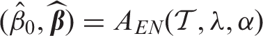
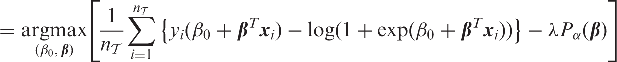
For the learning phase, we considered penalized logistic regression models from the elastic net (EN) class with varying L1 and L2 penalties.^30,31 Training and cross-validation was carried out using the glmnet package (version 2.0–13), which allowed for fast computations. ³¹ The EN algorithm maximizes the penalized conditional log-likelihood

$$({\hat{\beta }}_0,\hat{\mathbf{\beta }})=A_{\mathit{EN}}(\mathcal{T},\lambda ,\alpha )$$

$$={\text{argmax}}_{({\beta }_0,\mathbf{\beta })}[\frac{1}{n_{\mathcal{T}}}\sum _{i=1}^{n_{\mathcal{T}}}\{y_i({\beta }_0+{\mathbf{\beta }}^T\hspace{0.17em}\mathbf{x}\mathbf{i})-\text{log}(1+\text{exp}({\beta }_0+{\mathbf{\beta }}^T\hspace{0.17em}\mathbf{x}\mathbf{i}))\}-\lambda P_{\alpha }(\mathbf{\beta })]$$

where $\alpha \in [0,1],\lambda \in [0,\infty )$ are tuning parameters and the penalty term $P_{\alpha }(\mathbf{\beta })$ is given by

$$P_{\alpha }(\mathbf{\beta })=(1-\alpha )\frac{1}{2}\left|\right|\mathbf{\beta }\left|\right|22+\alpha \left|\right|\mathbf{\beta }\left|\right|{\hspace{0.17em}}_1=\sum _{p=1}^P[\frac{1}{2}(1-\alpha ){\beta }_p^2+\alpha \left|{\beta }_p\right|]$$

Predictions $\hat{y}\in \{0,1\}$ are obtained by thresholding the predicted probability $1/(1+\text{exp}(-({\hat{\beta }}_0+{\hat{\mathbf{\beta }}}^T\mathbf{x})))$ for the event Y = 1 at 0.5.

For every learning data set $\mathcal{L}$ , we train M = 100 models by considering $\alpha =0,0.25,0.5,0.75,1$ and for each α, 20 equidistant values for λ in the interval $[{\lambda }_{min}(\alpha ),{\lambda }_{max}(\alpha )]$ . Hereby λ_min is close to zero and λ_max, for which $\hat{\mathbf{\beta }}=0$ depends on the training data. Details are provided in the glmnet documentation. ³² Expected performance estimates $({\hat{\vartheta }}_m(\mathcal{V}))m\in \mathcal{M}$ for all algorithms A _m are obtained via 10-fold cross-validation.

In the following, different heuristic selection rules based on the (cross-)validation performance estimates are defined.

default: evaluate only the best validation model

within 1 SE: evaluate all models with validation performance within one standard error of the best validation model

best 10%: evaluate the top 10% of models based on the validation ranking

no selection: evaluate all initial candidate models

Besides these four rules, we also consider the oracle selection rule defined as the (truly) best model. This rule can of course not be employed in practice but may serve as a benchmark. As the final simulation step, evaluation data $\mathcal{E}\sim {\mathfrak{D}}^{n_{\mathcal{E}}}$ is generated and the selected models are evaluated with the maxT-approach. We considered different evaluation sample sizes $n_{\mathcal{E}}\in \{100,200,400,800\}$ .

All results given in the following are averaged over all of N _sim  = 5000 performed simulation runs per scenario $(\stackrel{\sim }{\mathfrak{D}},n_{\mathcal{L}},\mathfrak{D},n_{\mathcal{E}})$ . For estimated proportions (FWER, Power) this implies a standard error of at most $\sqrt{0.25/5000}\approx 0.0071$ . We performed a paired comparison, meaning that evaluation strategies $\mathbf{\psi }=(\mathbf{r}\mathbf{,}\mathbf{\varphi })$ are applied to the same 5000 combinations of learning and evaluation datasets per scenario. For all trained prediction models, the true model performance ${\vartheta }_m$ is ‘calculated’ on a large population data set $\mathcal{P}\sim {\mathfrak{D}}^{n_{\mathcal{P}}}$ of size $n_{\mathcal{P}}=100,000$ with negligible numerical error.

3.2 Results

3.2.1 Prediction tasks

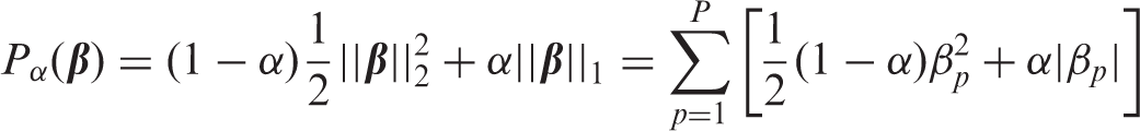
For $n_{\mathcal{L}}=200$ , Figure 2 visualizes the empirical distribution (over the 5000 simulations) of the optimal performance ${\vartheta }_{\mathit{opt}}=\underset{m\in \mathcal{M}}{max}{\vartheta }_m$ and the ‘median’ performance ${\vartheta }_{\mathit{med}}$ , defined as the empirical median of $\{{\vartheta }_m\}m\in \mathcal{M}$ . Additionally, the accuracy of the true (data generating) model is indicated. This can be seen as an illustration of how well the prediction tasks can be learned by the considered elastic net algorithm class for each of the eight learning tasks.

Figure 2.

Illustration of the optimal and median performance of the M = 100 candidate models over N _sim  = 5000 simulation runs for $n_{\mathcal{L}}=200$ stratified by prediction task. The diamond symbols indicate the performance of the data generating model.

As expected, performances are increasing in the effect sizes controlled by μ₁ and μ₂. In the following, we will only present our findings for scenario A $({\mu }_1=4,\rho =0)$ and B $({\mu }_2=6,\rho =0)$ in detail as highlighted in Figure 2. For $n_{\mathcal{L}}=200$ the mean optimal performances (over all simulations) are 92.4% and 88.0% for scenario A and B, respectively. Besides a slightly increased mean optimal performance (A: 93.4%, B: 89.6%) when training the models on $n_{\mathcal{L}}=400$ instead of 200 observations, model selection quality should also be superior in this case, since more validation data is available. Learning a good model for task A is easier with the considered class of algorithms in the sense that the optimal candidate model performance is on average closer to the theoretically achievable performance (A: 94.0%, B: 92.9%).

Note that only the within 1 SE rule selects a varying number $M^{*}$ of models while $M^{*}$ is constant for all other selection rules tested. The overall median $M^{*}$ over all scenarios is 8 with an interquartile range (IQR) of 9. For $n_{\mathcal{L}}=200$ , the median $M^{*}$ was 9 ( $\text{IQR}=7$ ) for scenario A and 6 ( $\text{IQR}=5$ ) for scenario B. As $M^{*}$ is on average close to 10, the results of the within 1 SE and the best 10% rules are quite similar in our simulation study. Consequently, we will only show the results for the within 1 SE rule to streamline the presentation.

3.2.2 Rejection rate

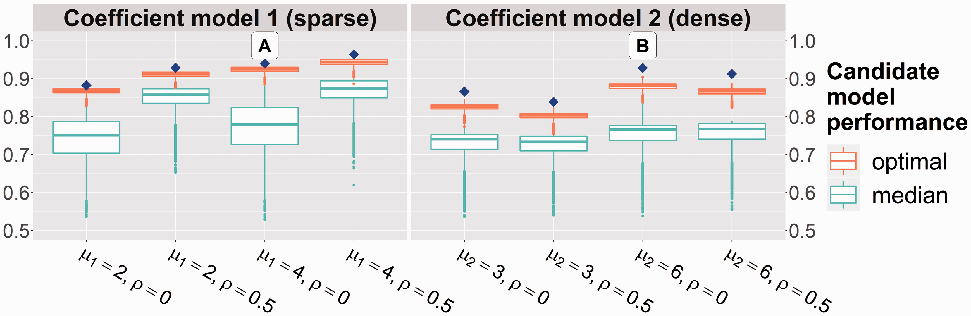
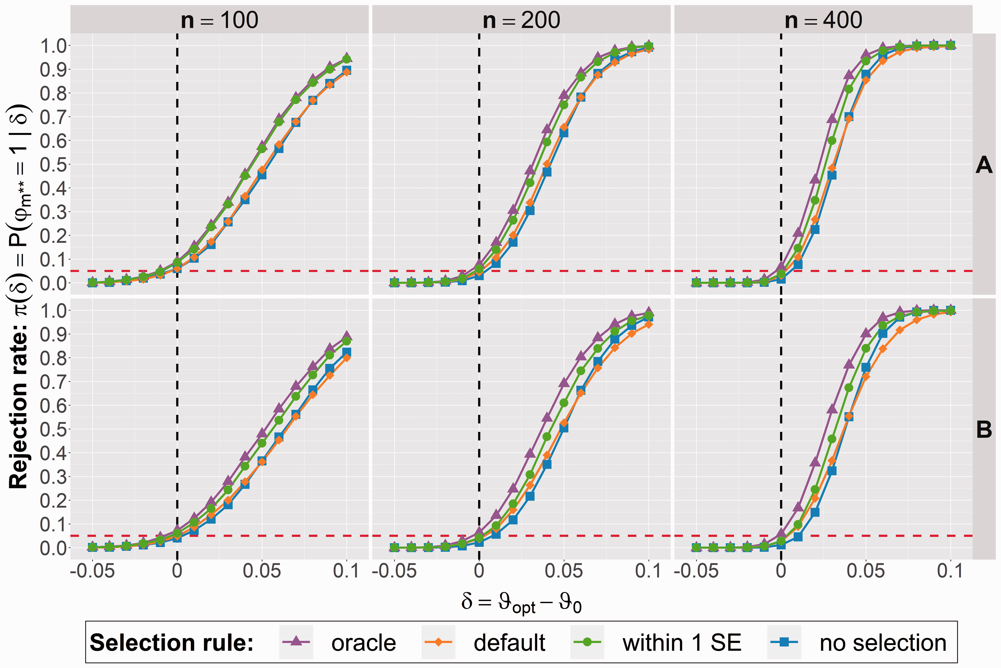
Figure 3 compares the different evaluation strategies regarding their overall rejection rate, i.e. the probability of a successful evaluation study. Here, the black vertical line represents the scenario ${\vartheta }_0={\vartheta }_{\mathit{opt}}=\underset{m\in M}{max}{\vartheta }_m$ , the maximum value of ${\vartheta }_0$ such that all null hypothesis $H_0^m,m\in \mathcal{M}$ , are still true. As pointed out above, the mean ${\vartheta }_{\mathit{opt}}$ is 92.4% for scenario A and 88.0% for scenario B. The value $\delta ={\vartheta }_{\mathit{opt}}-{\vartheta }_0$ describes if the global null G is true ( $\delta \le 0$ ) or false ( $\delta >0$ ).

Figure 3.

Rejection rate for the null hypothesis of the final model $m^{**}$ stratified by scenario (top: A, bottom: B) and evaluation sample size (from left to right: $n_{\mathcal{E}}=100,200,400$ ).

As described earlier we will select $m^{**}=\text{argma}{\text{x}}_{m^{*}\in {\mathcal{M}}^{*}}{T}_{m^{*}}$ as our final model based on the evaluation data. We consider $\pi (\delta )=\mathbb{P}({\varphi }_{m^{**}}=1|\delta )$ , the rejection rate for $H_0^{m^{**}}⋮{\vartheta }_{m^{**}}\le {\vartheta }_0$ , as most important. In practice, the evaluation study is declared successful if and only if ${\varphi }_{m^{**}}=1$ . For $\delta \le 0$ , a rejection of $H_0^{m**}$ is always wrong and π coincides with the FWER. The situation $\delta >0$ is more complex: a rejection of $H_0^{m**}$ is not automatically correct as we might have ${\vartheta }_{m**}\le {\vartheta }_0<{\vartheta }_{m*}$ for another $m^{*}\ne m^{**}$ . We found in separate analyses that the probability for a false rejection is maximal for δ = 0 and monotone decreasing in $\left|\delta \right|$ , as expected. Altogether $\pi (\delta )$ should be increasing in δ while being bounded by $\alpha =0.05$ for $\delta \le 0$ .

It can be observed that the within 1 SE selection rule uniformly outperforms the default strategy where only the best model from the evaluation stage is selected. The gain in terms of rejection rate is up to 10% in specific situations (depending on $n=n_{\mathcal{E}}$ and δ). On the other hand, when the candidate model set is not reduced at all based on the validation data (no selection), the rejection rate is commonly lower compared to the default approach. We confirmed through separate analyses that the increased rejection rate is not inflated by false-positive test decisions but rather represents a real power increase.

For lower samples sizes $n_{\mathcal{E}}<200$ , we observe an increased FWER up to 10% for δ = 0. Note that the default approach can also not control the type 1 error exactly, but the problem is less severe here.

3.2.3 Estimation bias

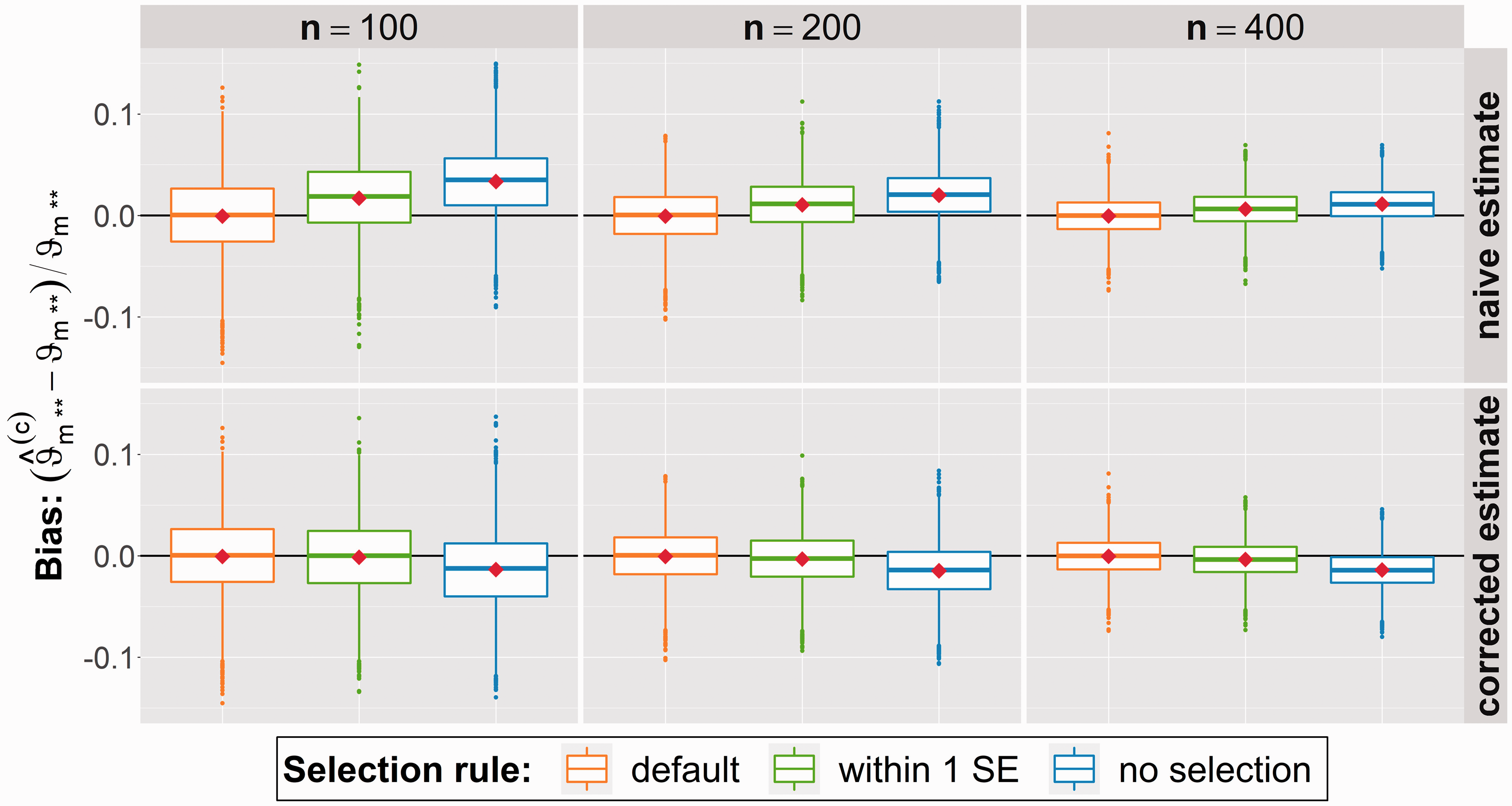
The price to pay for the increased power is the upward bias of the point estimate of the final model ${\hat{\vartheta }}_{m^{**}}$ . This can be seen in the upper part of Figure 4, which shows the distribution of the relative deviation $({\hat{\vartheta }}_{m^{**}}-{\vartheta }_{m^{**}})/{\vartheta }_{m^{**}}$ stratified by selection method for scenario B. This finding is not surprising, as one of the reasons to evaluate only one model (default approach) was to obtain an unbiased performance estimate for that model. Besides the regular point estimate ${\hat{\vartheta }}_{m^{**}}$ we also consider the alternative point estimate ${\hat{\vartheta }}_{m^{**}}^c$ defined in equation (17). The lower part of Figure 4 shows that the upward bias vanishes indeed due to this correction. On the other hand, when more (all) models are evaluated, we now rather observe a downward bias of the corrected estimate, which is also in line with our expectations as the corrected estimator is median-conservative.

Figure 4.

Relative deviation of the naive (top) and corrected (bottom) point estimate compared to the true value of the final model performance for scenario B and different evaluation sample sizes $n_{\mathcal{E}}$ . The diamond symbols indicate the sample means.

3.2.4 Final model performance

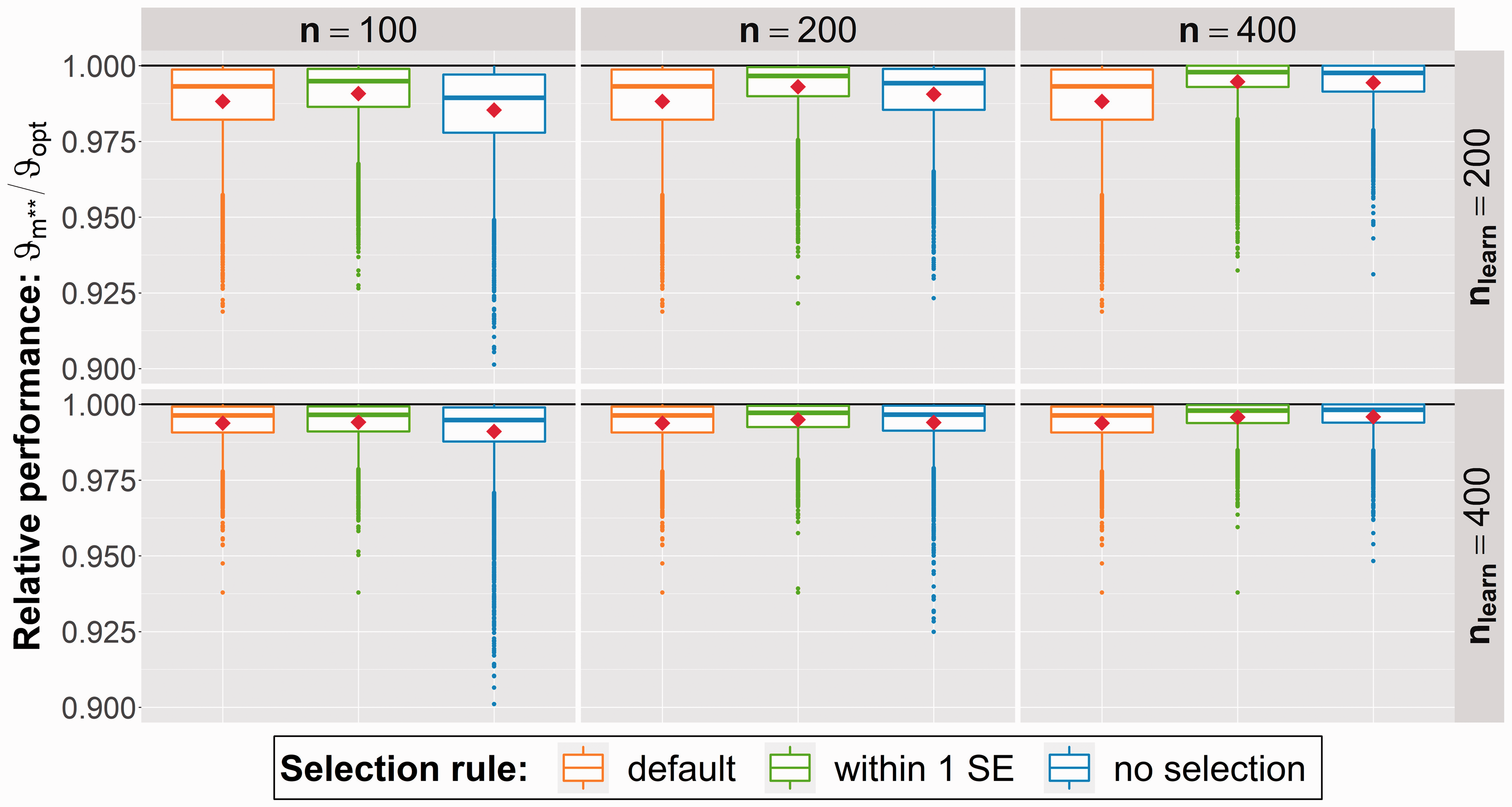
We also investigate the true performance of the final chosen model relative to the optimal performance ${\vartheta }_{\mathit{opt}}=\underset{m\in \mathcal{M}}{max}{\vartheta }_m$ , which is depicted for scenario B in Figure 5. Here the relative performance ${\vartheta }_{m^{**}}/{\vartheta }_{\mathit{opt}}$ is shown stratified for selection rule, learning sample size $n_{\mathcal{L}}$ and evaluation sample size $n=n_{\mathcal{E}}$ . As stated above, the true performance in our simulations is calculated as the sample average over a large population dataset with 100,000 observations.

Figure 5.

Distribution of final model performance ${\vartheta }_{m^{**}}$ relative to the optimal performance ${\vartheta }_{\mathit{opt}}=\underset{m\in \mathcal{M}}{max}{\vartheta }_m$ for learning task B. Results are stratified by evaluation sample size $n=n_{\mathcal{E}}$ (columns) and learning sample size $n_{\mathcal{L}}$ (rows).

We first note that all selection rules work well in the sense that the relative final performance is close to 100% on average. Interestingly, the expected final model performance when multiple models are evaluated is slightly higher. When more than a single model is evaluated, the expected model performance increases in the number of evaluation observations. This is plausible because the final model is selected based on these observations. When all models are evaluated (no selection rule), the performance is lower compared to the within 1 SE rule.

3.2.5 Learning from non-representative data

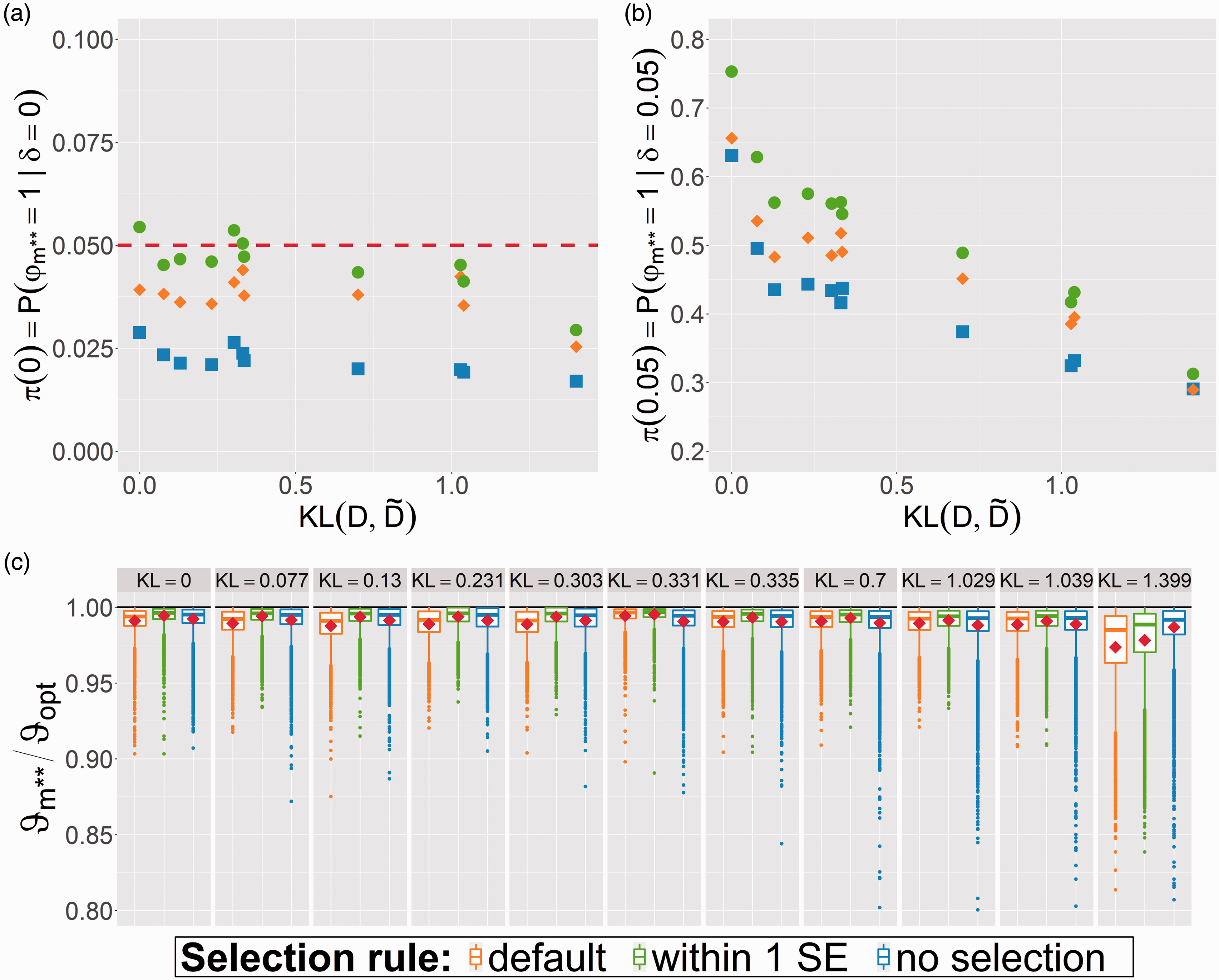
Finally, we consider the case when the learning data $\mathcal{L}\sim \stackrel{\sim }{{\mathfrak{D}}^{n_{\mathcal{L}}}}$ is sampled from an altered distribution $\stackrel{\sim }{\mathfrak{D}}$ compared to the target distribution $\mathfrak{D}$ for scenario A ( ${\mu }_1=4,\rho =0$ ). Figure 6 shows the rejection rate under the global null (Figure 6(a): $\delta ={\vartheta }_{\mathit{opt}}-{\vartheta }_0=0$ ) and under the alternative (Figure 6(b): $\delta =0.05$ ) where the likelihood to obtain an non-representative sample is measured as $\text{KL}(\mathfrak{D},\stackrel{\sim }{\mathfrak{D}})$ , the Kullback-Leibler (KL) divergence from $\stackrel{\sim }{\mathfrak{D}}$ to $\mathfrak{D}$ . ²⁶ (p.329). We observe that all evaluation strategies perform worse the larger $\text{KL}(\mathfrak{D},\stackrel{\sim }{\mathfrak{D}})$ becomes. Just as in the optimal case $\mathfrak{D}=\stackrel{\sim }{\mathfrak{D}}(\iff \text{KL}(\mathfrak{D},\stackrel{\sim }{\mathfrak{D}})=0)$ the within 1 SE rule clearly outperforms the default approach as well as the no selection strategy. Figure 6(c) shows the distribution of the final model performance. For all cases, except the one with the highest disturbance, the within 1 SE approach yields the highest expected performance ${\vartheta }_{m**}$ .

Figure 6.

Properties of selection rules when learning and evaluation population differ (measured via KL divergence from learning distribution $\stackrel{\sim }{\mathfrak{D}}$ to evaluation distribution $\mathfrak{D}$ ) for prediction task A. (a) Rejection rate under global null ( $\delta ={\vartheta }_{\mathit{opt}}-{\vartheta }_0=0$ ). (b) Rejection rate under alternative ( $\delta =0.05$ ). (c) Relative final model performance ${\vartheta }_{m^{**}}/{\vartheta }_{\mathit{opt}}$ .

3.2.6 Sensitivity analyses

The results for all other simulated prediction tasks (Figure 2) were similar to the presented results. In particular, the default approach was always outperformed by the within 1 SE selection rule with regards to rejection rate and final model performance. In addition, we repeated our analysis with 5-fold CV instead of 10-fold CV as a basis for the model selection in the learning stage (N _sim  = 2000). Despite the slightly higher bias of $\hat{\vartheta }(\mathcal{V})$ in this case, results were very similar to the results obtained when employing 10-fold CV.

3.2.7 Different learning algorithms

In our main simulation, all prediction models arise from the same learning algorithm, the elastic net, by variation of two hyperparameters. Another case of practical interest involves the comparison of several different learning algorithms on the same task. To mimic this case, we implemented the following additional simulation.

Instead of 100 elastic net models, 20 models were trained from each of the following five learning algorithms: elastic net, random forests, decision trees, support vector machines and extreme gradient boosting. We used existing implementations of these algorithms from the caret package (and according dependencies), by setting the training method to glmnet, ranger, rpartCost, svmLinearWeights2 and xgbTree, respectively. ³³ Additional details are provided in the web-based help for the caret package. ^b

These algorithms depend on two to seven hyperparameters which were sampled randomly according to the default caret implementation in this simulation. We limited this analysis to learning tasks A and B (compare Figure 2) due to the increased computational demand for training algorithms other than the elastic net. In addition, we used a simple hold-out validation rather than cross-validation to further reduce the computatinal burden of this study. Apart from these changes, the setup was exactly as described earlier for the main simulation. Overall, this simulation includes 5000 instances of the learning-evaluation pipeline per scenario $(\mathfrak{D},n_{\mathcal{L}},n_{\mathcal{E}})$ .

In summary, the results concerning this sensitivity analysis qualitatively match the main results. The power when employing the within 1 SE rule is strictly greater than for the default approach. This is true for all sample sizes and both learning tasks resulting in graphs highly similar to Figure 3. On the other hand, the type 1 error rate is also slightly increased. In contrast to the main simulation, the type 1 error was controlled at the nominal level α in all cases for both selection rules, even for the smaller evaluation sample sizes. Concerning estimation bias and the expected final model performance, the results were again very similar to those reported in Figures 4 and 5, respectively.

4 Application to real data

Finally, we illustrate our simultaneous model evaluation strategy on real data. For this purpose, we use the Breast Cancer Wisconsin (Diagnostic) Data Set ^c and the Cardiotocography Data Set ^d which are both freely accessible at the UCI Machine Learning Repository. ³⁴ Details regarding these datasets are given by Street et al. ³⁵ and Ayres-de Campos et al., ³⁶ respectively. Both our analyses are briefly described in the following and are fully reproducible as the corresponding R code is publicly accessible.^a Our primary goal here is not to come up with a superb prediction model, but rather illustrate how multiple models can be evaluated simultaneously and results shall be interpreted. Similar to our simulation study, we consider M = 100 penalized logistic regression candidate models from the elastic net class for each learning task.^30,31 We will employ the within 1 SE selection rule.

4.1 Diagnosis of breast cancer

This dataset contains of 569 observations of 30 numerical features which “are computed from a digitized image of a fine needle aspirate (FNA) of a breast mass. They describe characteristics of the cell nuclei present in the image.” ³ Features describe texture, area and spatial structure, among others. Our learning task is to predict breast cancer, which is the given label for 212 out of the 569 available instances. We randomly split the dataset into $n_{\mathcal{L}}=427$ observations for learning and $n_{\mathcal{E}}=142$ samples for evaluation.

In the learning phase, the 100 candidate models are compared by means of 10-fold CV. The best model is one with zero L1 penalty and hence all 30 model coefficients (not counting the intercept) are nonzero. It achieves a CV accuracy of 97.2%. Two further models with only 13 and 8 nonzero coefficients fall within one standard error of the best model. Hence we obtain a total of $M^{*}=3$ selected models for the evaluation phase.

In the evaluation study, we observe uncorrected performance estimates of $137/142\approx 96.5\%$ for two of the models and 95.8% for the last model. As our usual strategy to simply pick the best model leads to a tie, we decide to favor the more parsimonious model (eight nonzero coefficients) over the saturated model (30 nonzero coefficients). For this final model, we obtain a corrected performance estimate of 95.8% and a lower 95% confidence limit of 93.4% via the maxT-approach; compare equations (17) and (12). If our goal was to reject the null hypothesis of a performance less or equal to 90% with a FWER of 5%, we should do so based on this evidence.

4.2 Prediction of abnormal fetal state

The second dataset contains 2126 fetal cardiotocograms (CTGs). “They were automatically processed and the respective diagnostic features measured. The CTGs were also classified by three expert obstetricians and a consensus classification label assigned to each of them.” ⁴ Our learning task is to predict a suspect or pathologic fetal state (295 + 176 instances) versus a normal state (1655 instances). The 24 features include diverse properties of the fetal heart rate histogram. As with the breast cancer data we employ a 3:1 ratio for the splitting into learning and evaluation data. However, since each observation has an associated measurement date, we learn on the first $n_{\mathcal{L}}=1594$ and evaluate on the last $n_{\mathcal{E}}=532$ instances, mimicking the real life condition of time delay between the two phases. The date attribute was not used for model devolopment.

In the learning phase, the best cross-validation performance is 93.5% obtained by a rather sparse model with eight nonzero coefficients. In this case, seven additional models with 6 to 23 nonzero coefficients are within one standard error of the best model and hence selected for evaluation. Based on these intermediate results, one may seek to obtain a final model with an accuracy greater than ${\vartheta }_0=0.8$ .

In the evaluation study, empirical performances of the $M^{*}=8$ selected models range between 72.9% and 79.5%. The performances dropped significantly from learning to evaluation phase, hinting at systematic differences due to the different sampling time periods. Interestingly, the best validation model performs worst among the selected models on the evaluation data. For the best evaluation model, which also has eight nonzero coefficients, we obtain a corrected accuracy estimate of 78.7% and a lower confidence limit of 75.9%. Hence, the null hypothesis $H_0⋮{\vartheta }_{m^{**}}\le 0.8$ cannot be rejected. This example clearly illustrates the advantage of the proposed within 1 SE strategy although unlike in our simulations the ground truth is not known: If we would have used the default selection approach and thus decided on the final model based only on the validation data, the final estimated performance would have been only 72.9%. The lower confidence limit would have been $69.7\%=0.729-1.645·\sqrt{0.729·(1-0.729)/532}$ .

5 Discussion

5.1 Conclusions

This work shows that the simultaneous evaluation of multiple predictions is feasible and false positive claims regarding model performances can be controlled. This is achieved via a multiple test that (asymptotically) controls the family wise error rate, i.e. the probability to make at least one false positive test decision. In this work, we applied the maxT-approach as one possibility of such a multiple test. Its main advantage is to explicitly take into account the similarity of models in terms of the correlation between performance estimates. This reduces the necessary adjustment for multiplicity compared to simpler methods like the Šidák correction if the evaluated models give similar predictions. The maxT-approach is applicable in a wide context, most importantly when the empirical performance estimate (sample average) is used. This also applies to performance measures for regression tasks. Other measures may also be used as long their estimators approximately follow a multivariate normal distribution, as it is for instance the case for the (nonparametric) area under the curve (AUC) estimator. ³⁷ As we have only conducted simulations regarding classification accuarcy, the operating characteristics of the multiple testing approach (FWER, power, estimation bias) may deviate from our results for other performance measures.

One major advantage of selecting multiple models for evaluation is the higher power, i.e. the increased probability to correctly identify a model that performs sufficiently well. Employing this approach will therefore lead to evaluation studies that are more likely to be successful or, equivalently, need less observations per study to achieve the same power. This is relevant when the sample sizes cannot be too large due to cost constraints or ethical considerations, which is often the case in medical research. Luckily, the main drawback of the procedure, namely the overoptimistic estimation of the final model performance, can be negated by means of a corrected point estimator. This is another major benefit of the maxT-approach and not easily possible for simpler methods like the Šidák correction.

Based on our results, we recommend to select all models for evaluation which are close to the best model based on the validation estimates, e.g. within one standard error. As seen in our numerical experiments, this strategy outperforms the default approach regarding power and also slightly improved the final model performance. This conclusion is still valid in the suboptimal but realistic case when learning and evaluation distributions are not identical but rather differ systematically. Although we could not yet derive precise conditions under which our approach is superior, our results can intuitively be explained as follows. First, any selection rule can be seen as a compromise between the default approach (evaluate only best validation model) and the no selection approach (evaluate all models). In these two extreme cases model, selection is conducted completely in either the validation phase or the evaluation phase. However, when a subset of models is (pre-)selected based on the validation ranking and the final model is selected based on the evaluation data, effectively more data is used for the model selection.

Apart from the power increase, the performance of the final model also improves when employing the within 1 SE selection rule compared to the default approach. Albeit the magnitude of this effect was rather small in our simulations, this performance improvement comes with no additional cost in the sense that the FWER can still be controlled (asymptotically). In this regard, our evaluation strategy can be seen as a way to improve model selection by incorporating the evaluation data without introducing over-optimism.

5.2 Limitations

Our simulation results are meaningful but strictly speaking limited to the considered (true) model performances ϑ and the correlation structure $\mathbf{R}$ between performance estimates. However, these might also occur when other candidate model types than the elastic net class is considered. The results remained qualitatively the same when considering a more diverse collection of learning algorithms to train the prediction models. The according simulation study was, however, smaller in scope. We plan to extend our numerical experiments regarding several aspects such as the prediction tasks and employed learning algorithms even further in the future.

The only true limitation of the maxT-approach is the loss of exact FWER control for lower evaluation sample sizes due to the asymptotic nature of this procedure. We observed an increased FWER of up to 10% (instead of the targeted $\alpha =0.05$ ) for low evaluation samples sizes around $n_{\mathcal{E}}=100$ . The same problem, however, also applies to the default approach where only one model was selected, due to the used normal approximation of the binomial distribution of θhat. This can be seen when comparing the default with the oracle selection rule (Figure 3): the default approach is only closer to the target level $\alpha =0.05$ because of imperfect model selection. A simple approach to alleviate this problem is to apply a transformation to the performance estimates, e.g. the logit transform and to apply the (multivariate) delta method. This reduced the FWER slightly (by around 2%) in ancillary simulations not shown here in detail. If strict FWER for low evaluation sample sizes is needed, we suggest to replace the maxT-approach by an exact (non-asymptotic) multiple test which is appropriate for the considered performance measure.

We remark that under least favorable parameter configurations, i.e. when all evaluated models have the same true performance equal to the benchmark ${\vartheta }_0$ , the control of the type 1 error will get worse when more models are included. This is, however, also an increasingly unlikely scenario. For the most extreme case when all initial candidtate models are evaluated (no selection rule), we observed a rejection rate below the nominal level (Figure 3) due to considerably different true parameter values (Figure 2).

5.3 Outlook

Although the simultaneous evaluation of multiple prediction models worked great in our simulations, there is no theoretical guarantee to obtain a certain power increase, with the selection rules we employed. This leads to the question of optimal selection rules. For instance, one could explicitly take estimates for performance and correlation structure from the validation data into consideration in order to maximize the expected power. We encourage further research in this direction.

In practice, it may of course be necessary to also consider other factors besides raw predictive performance. In this regard, an appropriate strategy would be to formulate and check suitable side conditions before the evaluation study. For instance, an implausible or overcomplex model might not be considered for evaluation even if the empirical validation performance is high.

A common approach in machine learning is to combine different models into a single ensemble model. Different techniques exist in this regard, e.g. bagging or boosting. ⁶ As they can also be seen as the output of a learning algorithm, ensemble models are technically already covered in our multiple testing framework. Our smaller ancillary simulation also covers boosted trees as an example of such an ensemble technique. An interesting question for future work would be to compare the efficieny in terms of statistical power (and final model performance) of (a) the selection of multiple promising models for evaluation and (b) averaging (weighting) these models to get a single ensemble model which will then be evaluated.

Our work sheds new light on the question how to optimally allocate observations to the training, validation and evaluation datasets. This issue has received some attention in the past. ³⁸ The statistical power of the evaluation study was, however, not considered as an important property of the machine learning and evaluation pipeline. As a general guideline, we recommend that a power estimation should precede any evaluation study, see equation (13). In the best case, the evaluation study is conducted prospectively and hence it can be decided (within certain bounds) how many observations need to be acquired. In case the estimated power is low even under ideal conditions (maximum acquirable sample size, optimistic assumptions regarding true performance(s)), we would refrain from conducting a formal evaluation study and consequently from making strong claims about the predictive performance.

For classification tasks, accuracy is seldom used alone as a single performance measure. Instead, at least in medical diagnostic accuracy studies, sensitivity and specificity are defined to be co-primary endpoints. In this case, the statistical inference problem is more complex and there are more options for model selection during validation and evaluation phase which will be compared systematically in the future.