Bayesian estimation of the binomial parameter in sequential experiments

Abstract

This article presents an objective Bayesian approach to estimating the binomial parameter in group sequential experiments with a binary endpoint. The idea of deriving design-dependent priors was first introduced using Jeffreys criterion. Another class of priors was developed based on the reference prior theory. A theoretical framework was established showing that explicit reference to the experimental design in the prior is fully Bayesian justified. Using a design-dependent prior which generalizes the reference prior, I propose a comprehensive and unified approach to the point and the interval estimations in group sequential experiments, and I evidence the good frequentist properties of the posterior estimators through comparative studies with the existing methods. The effect of the prior correction on the posterior estimates is studied in three classical designs of clinical trials. Finally, I discuss the idea of using this approach as a default choice for estimation upon sequential experiment termination.

1. Introduction

In the experimental context, the benefits of stopping early can be ethical as well as purely economic. Group sequential designs have become commonplace across all phases of the clinical development. The reasons for an early stopping may be related to efficacy (i.e. strong evidence of the treatment effect) or futility (i.e. absence of treatment effect). In frequentist sequential designs, the adjustments to the stopping boundaries are concerned with controlling the overall type I error rate of a testing procedure. Examples of such adjustments include the Pocock ¹ and the O’Brien–Fleming ² methods, and the error spending approach.^3,4 In Bayesian sequential design, the stopping rule can be based on posterior probability, posterior predictive probability, or a decision-theoretic framework.^5–7 Some of these Bayesian designs allow a control of the overall Type I error rate as well. ⁸

As a consequence of the influence of the stopping rule, group sequential designs tend to overestimate the true treatment effect if the trial stops early for efficacy. This trend was observed in a systematic review of clinical trials in cardiology, cancer, and immunodeficiency. ⁹ In another systematic review, authors noted that the published results often fail to adequately report relevant information about the decision to stop early, and sometimes show implausibly large treatment effects. ¹⁰ Authors also suggested that clinicians should view the results of such trials with skepticism. A reason for this caution is that most of the research undertaken has focused on the study designs and the associated question of maintaining the Type I error. ¹¹ In contrast, the question of the estimation of the treatment effect has received comparatively less attention, as reflected in the recent food and drug administration guidance on adaptive designs ¹² which states: “Biased estimation in adaptive design is currently a less well-studied phenomenon than Type I error probability inflation.”

Nonetheless, the issue of the estimation upon sequential experiment termination has given rise to an abundant literature. The influence of multiple looks at data on the maximum likelihood estimator ( $MLE$ ) is known for a long time ¹³ along with the deficiencies of the coverage probability of the Wald confidence interval ¹⁴ and the Bayesian credible intervals. ¹⁵ Various methods have been proposed by authors to estimate the binomial parameter in group sequential experiments with binary endpoint.

The frequentist solutions require ordering the observation space. The reason is that in the binomial case the complete and sufficient statistic is the couple of variables ( $S$ , $Y$ ) obtained upon stopping, where $S$ is the stopping stage and $Y$ is the experiment outcome which is often the accrued number of successes or responses to a therapeutic intervention. A widely known approach is based on the stage-wise ordering in which results corresponding to earlier termination are more extreme than those which terminate later. ¹⁶ However, pre-ordering the observation space introduces some subjectivity in the inference. ¹⁷ Other criticisms are that the solutions are not unique and may depend on the information levels for future (unobserved) stopping stages.

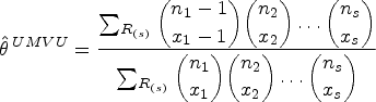
A uniformly minimum variance unbiased estimator ( $UMVUE$ ) can be derived using Rao–Blackwell’s theorem which states that, given an unbiased estimator and a sufficient and complete statistic, the conditional expectation of the first to the second is UMVU. Accordingly, the conditional expectation of the (unbiased) $MLE$ based on the first stage data given ( $S$ , $Y$ ) is $\mathrm{UMVU}$ . ¹⁸ Another point estimator consists of adjusting the $MLE$ by subtracting the estimate of its bias. ¹⁹ The bias is calculated at the adjusted $ML$ estimate using recursive method.

On the Bayesian side, the idea of deriving design-dependent priors was first introduced using Jeffreys’ criterion. ²⁰ A Bayesian prior is objective if it has minimal impact on the posterior distribution. In line with this principle, another class of design-dependent priors was developed based on the reference prior theory.^21,22 Both the Jeffreys and the reference priors coincide in the one-parameter case. Finally, a design-dependent prior conjugate to the binomial likelihood, namely the beta- $J$ prior, was derived for estimation problems based on an extension of the reference prior. ²³

In this article, I propose a comprehensive and unified approach to the point and the interval estimations of the binomial parameter based on the beta- $J$ prior. The method allows a correction for the influence of the stopping rule and applies to any one-arm experiment with a pre-specified stopping rule. The frequentist properties of the posterior estimators are evaluated and compared with the existing methods. The influence of the stopping rule and the effect of the prior correction on the point and the interval estimates are studied in three classical two-stage designs of clinical trials in oncology to test the rate of response to a therapeutic intervention. These are the Simon design ²⁴ which allows an early stopping for futility, the Pocock design which allows an early stopping for efficacy, and the O’Brien–Fleming design which allows an early stopping for either futility or efficacy. The estimates obtained using the new approach are compared with the existing alternatives, and recommendations are made about which of them provides results with acceptable interpretation in the experimental practice.

The next section presents key aspects of the reference prior theory in group sequential experiment. In Section 3, I describe the point and the interval estimators and their frequentist properties are investigated. The influence of the experimental design and the effect of the prior correction on the posterior estimates are studied in Section 4. In the conclusion, Section 5, I discuss the idea of using the new approach as a default choice for estimation upon experiment termination. Some technical details to derive the reference prior in sequential experiment are provided in the appendix in Supplemental Material. This document also contains results of simulations to assess the effect of the prior correction on the posterior estimators as the sample size varies and R scripts to produce results reported in this article along with some computational details.

2. Derivation of the reference prior

2.1. Reference prior theory

Descriptions of the reference prior theory and didactic tutorials can be found in the literature.^25,26 This section presents some key aspects of the derivation of the reference prior in group sequential experiment while more technical details are given in Section 1 of the appendix in Supplemental Material.

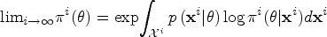
Let us consider $X$ the outcome variable and $\theta$ the model parameter, together with the prior specification $\pi (\theta )$ . The idea behind reference prior is to maximize a distance between the prior and the posterior distributions as data are collected. Formally, the data have maximum influence on the posterior if the Kullback–Leibler (K-L) divergence is maximum. By considering the expectation of the K-L divergence, the reference prior can be defined based on virtual data before experiment.

Let us consider the $i$ -dimensional vector ${\mathbf{\text{x}}}^i$ with density $p({\mathbf{\text{x}}}^i|\theta )$ and consider also the inferential scenario in which the components of ${\mathbf{\text{x}}}^i$ are $i$ realizations of $X$ from independent experiments. Asymptotic theory makes it possible to obtain a convenient form of the reference prior. The problem is reduced to computing:

$${\text{lim}}_{i\to \mathrm{\infty }}{\pi }^i(\theta )=\text{exp}{\int }_{{\mathcal{X}}^i}p({\mathbf{\text{x}}}^i|\theta )\text{log}{\pi }^i(\theta |{\mathbf{\text{x}}}^i)d{\mathbf{\text{x}}}^i$$

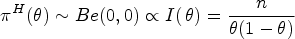
An analytical solution can be found using the Bernstein Von Mises theorem, sometimes called the Bayesian central limit theorem. It comes that, in the one-parameter problem, the reference prior is identical to the Jeffreys prior, noted ${\pi }^J(\theta )$ , obtained using Jeffreys’ criterion. If we denote by $I(\theta )$ the expected Fisher information, we have:

$${\pi }^R(\theta )\propto {\pi }^J(\theta )\propto I(\theta {)}^{\frac{1}{2}}$$

(1)

We now assume that the data are collected in a $K$ -stage experiment whose the design is noted $d_K$ . In the general case, the experiment outcome is obtained from a sequence of outcome values observed at the interim analyses, and the analysis times are predefined according to the statistical information available at each analysis. We consider a sequence of outcomes $x_{(s)}=(x_1,x_2,\dots ,x_s)$ observed until experiment termination and we assume that the density of $X_{(s)}$ is known. The likelihood function in the design $d_K$ takes the form:

$$L(\theta ;x_{(s)},d_K)={[L(\theta ;x_1)]}^{1_{s=1}}\times {[L(\theta ;x_{(2)})]}^{1_{s=2}}\times \cdots \times {[L(\theta ;x_{(K)})]}^{1_{s=K}}$$

(2)

Based on (2), the expected design-dependent Fisher information $I(\theta |d_K)$ can easily be expressed as a function of its naive (i.e. not design-dependent) counterpart:

$$I(\theta |d_K)=-E_{\theta }[\frac{{\mathrm{\partial }}^2}{{\theta }^2}\text{log}L(\theta ;x_{(s)},d_K)]=I(\theta )E_{\theta }(S)$$

(3)

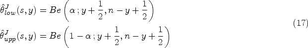
The introduction of the design information in the reference prior implies rewriting (1) as a function of $I(\theta |d_K)$ so that:

$${\pi }^R(\theta |d_K)\propto {\pi }^J(\theta |d_K)\propto I(\theta |d_K{)}^{\frac{1}{2}}$$

Jeffreys’ criterion applied to the likelihood (2) yields an expression of the design-dependent reference prior which depends on the naive Jeffreys prior and the expected stopping time:

$${\pi }^R(\theta |d_K)\propto {\pi }^R(\theta )E_{\theta }{(S)}^{\frac{1}{2}}\propto {\pi }^J(\theta )E_{\theta }{(S)}^{\frac{1}{2}}$$

(4)

Thanks to the component $E_{\theta }{(S)}^{\frac{1}{2}}$ in (4), the prior ${\pi }^R(\theta |d_K)$ reflects the degree of certainty associated with the projected design $d_K$ by over-weighing the probabilities about $\theta$ values more likely leading to late termination. The greater the certainty about $\theta$ values, the higher their prior probabilities. By so counterbalancing the expected effect of an early stopping, the reference posterior estimators benefit from a correction for the influence of the stopping rule. These properties were recently evidenced in the normal case. ²⁷

2.2. Theoretical framework

Taking into account data-dependent stopping rule in experiment has long been a source of controversies among theoretical statisticians. Some are reluctant to transgress the stopping rule principle according to which once the data have been obtained, the reasons for stopping the experiment should have no bearing on the evidence reported about the parameter. The stopping rule principle is the main consequence of the likelihood principle which states that all of the information about the parameter provided by an experiment outcome is expressed in the likelihood function. In turn, the likelihood principle is considered as a direct implication of Bayes’ theorem. However, any applied statistician considers that the design information cannot be ignored because of the bias induced by the stopping rule.

An important breakthrough was made by showing that Bayes’ rule can be expressed with an explicit reference to the experimental design $d_K$ . ²⁸ Consequently, the likelihood principle is no longer a direct implication of Bayes’ rule. Let us assume that the sequence of independent outcomes $x_{(k)}=(x_1,x_2,\dots ,x_k)$ has a known density function $p(x_{(k)}|\theta )$ which satisfies minimum conditions of regularity, Bayes’ rule becomes:

$$\pi (\theta |x_{(k)},d_K)\propto \pi (\theta |d_K)p(x_{(k)}|\theta ,d_K)$$

(5)

Formulation (5) holds for any group sequential experiment governed by a proper stopping rule. On this basis, any posterior estimator derived using the design-dependent reference prior (4) is fully Bayesian justified. It also becomes evident that a state of prior ignorance cannot be characterized without reference to the experimental design and Bayesian objectivity cannot ignore such information.

3. Posterior estimators in sequential experiments

3.1. Reference prior in the binomial model

In the one-parameter case, the reference prior is obtained via a straightforward application of Jeffreys’ criterion. Let $d_{BinK}$ denote a $K$ -stage design ( $K\ge 2$ ), where $x_{(k)}=(x_1,x_2,\dots ,x_k)$ is now a sequence of successive binomial trials of fixed sizes $n_k$ ( $k=1,\dots ,K$ ) and $\theta$ is the binomial parameter. At stage $k$ , the available data are analyzed and a decision whether to continue or to stop the experiment is made based on the accrued number of successes $y_k=\sum _{i=1}^k{x}_i$ . Let us introduce $J_k$ ( $k=1,\dots ,K-1$ ) which is the continuation region to stage $k+1$ for $y_k$ . So, the stopping stage $S$ is the first $k$ such that $y_k\notin J_k$ , and the stopping rule is determined by

$$P_{\theta }(S\ge k)=P_{\theta }(Y_1\in J_1,Y_2\in J_2,\dots ,Y_{k-1}\in J_{k-1})$$

(6)

which is obtained by summing the probabilities

$$p(x_{(k-1)}|\theta ,d_{BinK})={\displaystyle (\genfrac{}{}{0ex}{}{n_1}{x_1})}\dots {\displaystyle (\genfrac{}{}{0ex}{}{n_i}{x_i})}{\theta }^{y_i}(1-\theta {)}^{n_1+\cdots +n_i-y_i}$$

in the $k-1$ dimensional restriction

$$R_{(k-1)}=\{x_{(i)}:y_i\in J_i;i=1,\dots ,k-1\}$$

(7)

The restriction $R_{(k-1)}$ in (7) contains all the sequences $x_{(k-1)}$ (or paths) such that all the outcome values $y_i$ ( $i=1,\dots ,k-1$ ) allow the continuation of the experiment to stage $k$ . Each interval $J_i\ni y_i$ can be determined based on a given limit value for the observed rate or on a $p$ -value if a frequentist testing procedure is planned. In this case, each $J_i$ contains the values of $y_i$ not rejecting an hypothesis, usually the null hypothesis. Practical examples in clinical trials are given in Section 4. In experimental science, it is also common to use designs based on the beta posterior distribution of the parameter wherein the experiment stops, for example, if a given accuracy level which is specified by the credible interval length is reached. Accordingly, each interval $J_i$ contains the values of $y_i$ satisfying the continuation criterion. Other Bayesian designs are based on the posterior predictive distribution of future observations. Therefore, the values of $y_i$ in $J_i$ are determined according to the beta-binomial probabilities of the future outcome values.

Based on (3), the expected Fisher information conditional on the design $d_{BinK}$ in the binomial model takes the form:

$$I(\theta |d_{BinK})=\frac{1}{\theta (1-\theta )}{E}_{\theta }(S)$$

(8)

The design-dependent reference prior can now be expressed in function of the naive $Be(\frac{1}{2},\frac{1}{2})$ prior distribution, as stated in (4), so that:

$${\pi }^R(\theta |d_{BinK})\sim {\theta }^{-\frac{1}{2}}(1-\theta {)}^{-\frac{1}{2}}{E}_{\theta }{(S)}^{\frac{1}{2}}$$

(9)

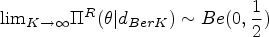
The properties of the reference prior (9) were first evidenced in the $K$ -stage Bernoulli design. ²⁹ In the Pascal (or inverse Bernoulli) sampling model, Jeffreys’ criterion results to the improper prior distribution $Be(0,\frac{1}{2})$ . This improper prior can be approached asymptotically by the proper reference prior (9) in the $K$ -stage Bernoulli design using truncation method. A formal proof of the correction for the stopping rule bias is outlined below.

Let us consider the $K$ -stage Bernoulli design $d_{BerK}$ for an experiment based on successive Bernoulli trials $x_k=0,1$ ( $k=1,\dots ,K$ ) with early stopping if the outcome is observed (i.e. $x_k=1$ ). The stopping rule (6) in the design $d_{BerK}$ simplifies to $P_{\theta }(M\ge k)=(1-\theta {)}^{k-1}$ . The Pascal sampling model describes the distribution of the outcome in the design $d_{BerK}$ when $K\to \mathrm{\infty }$ , and the associated stopping rule is infinite (i.e. $P_{\theta }(S<\mathrm{\infty })\ne 1$ a.s. when $\theta \to 0$ ). Formally, the stopping stage $S^{\prime }=inf\{k:X_k=1\text{ or }k=K\}$ in the design $d_{BerK}$ is a truncation of the stopping stage in the Pascal sampling model.

The reference prior (9) in the design $d_{BerK}$ becomes:

$$\begin{array}{rl}{\mathrm{\Pi }}^R(\theta |d_{BerK})& \propto {\theta }^{-\frac{1}{2}}(1-\theta {)}^{-\frac{1}{2}}(1+(1-\theta )+\cdots +(1-\theta {)}^{K-1}{)}^{\frac{1}{2}}\\ & ={\theta }^{-\frac{1}{2}}(1-\theta {)}^{-\frac{1}{2}}{\left(\frac{1-(1-\theta {)}^K}{\theta }\right)}^{\frac{1}{2}}\end{array}$$

(10)

When $K\to \mathrm{\infty }$ , the proper density of the reference prior for the design $d_{BerK}$ tends to the improper reference prior in the Pascal sampling model, that is,

$${\text{lim}}_{K\to \mathrm{\infty }}{\mathrm{\Pi }}^R(\theta |d_{BerK})\sim Be(0,\frac{1}{2})$$

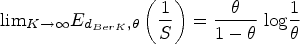
Compared to the naive $Be(\frac{1}{2},\frac{1}{2})$ prior distribution, ${\pi }^R(\theta |d_{BerK})$ in (10) assigns higher probabilities to the low values of $\theta$ as $K$ increases. It is easy to show that the prior correction is proportional to the bias induced by the stopping rule on the $MLE$ , which is ${\hat{\theta }}^{ML}=1/S$ . The bias of the $MLE$ is:

$$E_{d_{BerK},\theta }\left(\frac{1}{S}\right)-\theta =\sum _{k=1}^K(1-\theta {)}^{k-1}\theta \frac{1}{k}-\theta =\sum _{k=2}^K(1-\theta {)}^{k-1}\theta \frac{1}{k}>0$$

(11)

The bias increases as $K$ increases and reaches its maximum when $K\to \mathrm{\infty }$ or equivalently in the Pascal sampling model. The maximum bias is the limit of the geometric progression in (11) which is:

$${\text{lim}}_{K\to \mathrm{\infty }}{E}_{d_{BerK},\theta }\left(\frac{1}{S}\right)=\frac{\theta }{1-\theta }\text{log}\frac{1}{\theta }$$

3.2. Point estimation

In the Bayesian setting, the point estimators are often derived in relation to some given loss functions. Let $L(\theta ,{\theta }^{*})$ be the loss incurred in estimating $\theta$ when the estimate is ${\theta }^{*}$ . The quadratic loss $L(\theta ,{\theta }^{*})=(\theta -{\theta }^{*}{)}^2$ is a common loss function. The strategy is to find out a value of ${\theta }^{*}$ which minimizes the expected posterior loss, which is $h({\theta }^{*})=\int ({\theta }^{*}-\theta {)}^2\pi (\theta |x)d\theta$ . The condition for $h^{\prime }({\theta }^{*})=0$ is:

$${\theta }^{*}\int \pi (\theta |x)d\theta =\int \theta \pi (\theta |x)d\theta$$

(12)

Based on (12), $h({\theta }^{*})$ is minimized if the value of ${\theta }^{*}$ is the posterior mean, that is, ${\theta }^{*}=\int \theta \pi (\theta |x)d\theta$ . The mode of the posterior distribution is sometimes used as an alternative point estimator. This approach mimics the principle of likelihood maximization.

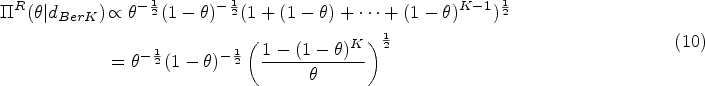
The beta- $J$ distribution, which is conjugate to the binomial likelihood, was defined in reference to the continuation regions $J_k$ in (6) to allow a flexible use of the components of the reference prior distribution in estimation problems. ²³ Its density contains the three components in $\theta$ of (9) and depends on the three positive scalars $a,b,c$ such that:

$$B{e}^J(a,b,c)\propto {\theta }^{a-1}(1-\theta {)}^{b-1}{E}_{\theta }{(S)}^c$$

(13)

If $c=0$ , (13) reduces to the beta distribution $Be(a,b)$ . Otherwise, if $c>0$ , posteriors are corrected for the influence of the stopping rule. The relation $a=b=c=\frac{1}{2}$ results in the classical form of the reference prior distribution.

We now examine the property of bias correction of priors based on the beta- $J$ distribution. In fixed $n$ -sample binomial experiment where $y$ is the observed outcome value, both the posterior mean based on the Haldane prior ${\pi }^H(\theta )\sim Be(0,0)$ and the posterior mode based on the uniform prior ${\pi }^U(\theta )\sim Be(1,1)$ coincide with the unbiased $MLE$ , which is ${\hat{\theta }}^{ML}=Y/n$ .

One can observe that the Haldane prior is proportional to the expected Fisher information, that is,

$${\pi }^H(\theta )\sim Be(0,0)\propto I(\theta )=\frac{n}{\theta (1-\theta )}$$

Extending this relationship to sequential experiments, we define the design-dependent version of the Haldane prior which is proportional to the expected Fisher information conditional on the design (8) so that:

$${\pi }^H(\theta |d_{BinK})\sim B{e}^J(0,0,1)\propto I(\theta |d_{BinK})$$

(14)

Relation (14) implicitly determines the value $c=1$ which is the extent to which the Haldane prior corrects for the stopping rule bias. This choice of the $c$ value may also apply to the design-dependent version of the uniform prior which we define as:

$${\pi }^U(\theta |d_{BinK})\sim B{e}^J(1,1,1)$$

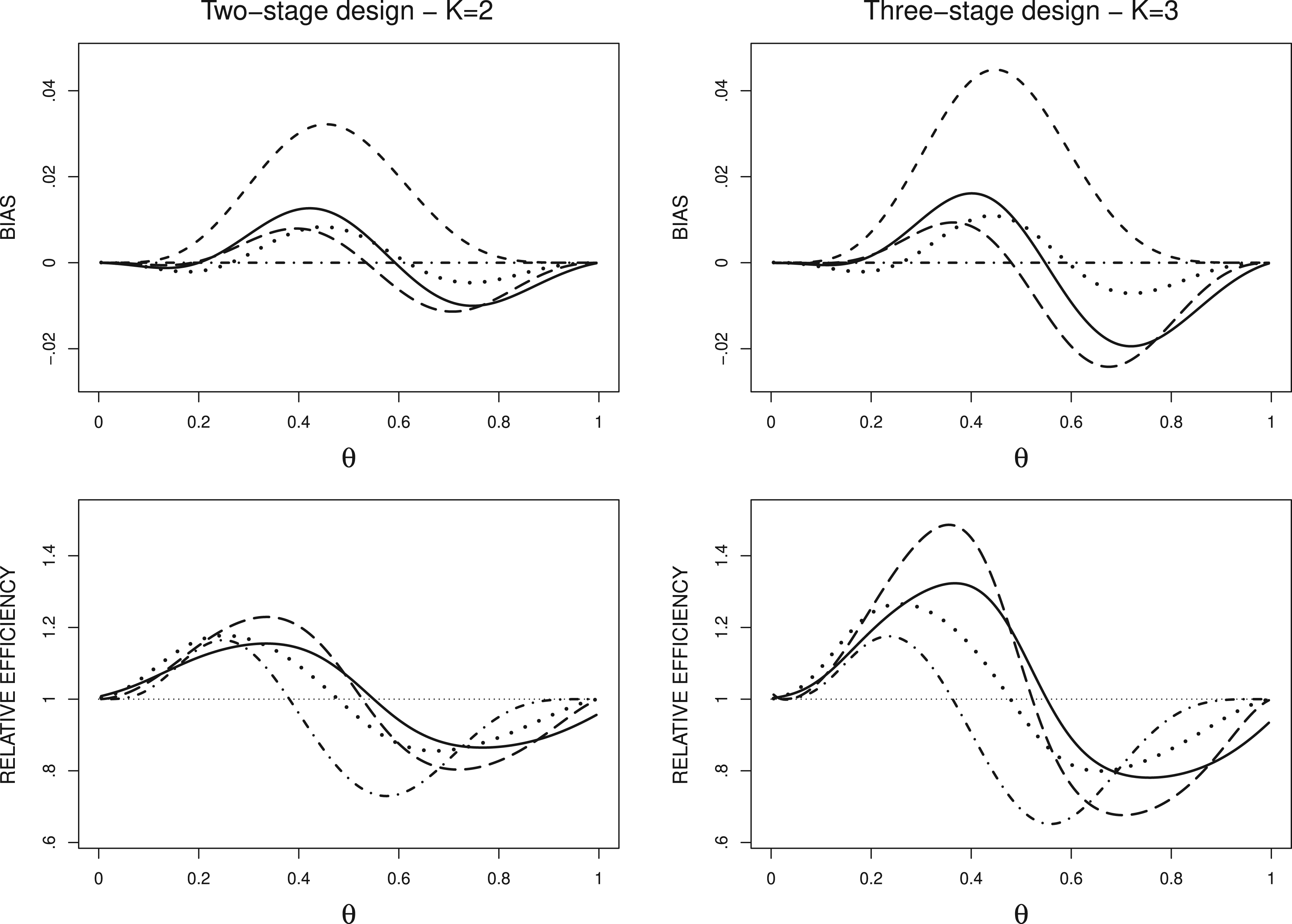
I now denote by $MEAN$ the estimator of the posterior mean based on the design-dependent Haldane prior and $MODE$ the estimator of the posterior mode based on the design-dependent uniform prior. In what follows, the biases of $MEAN$ and $MODE$ are studied in a two-stage and a three-stage design, namely $d_{BinK0.5}$ with $K=2,3$ , wherein the experiment is based on two or three successive samples of $10$ values and stops early if the $ML$ estimate is equal to or greater than 0.5. I also examine the efficiency relative to $MLE$ which is defined as

$$R{E}_{d_{BinK},\hat{\theta }}(\theta )=\frac{MS{E}_{d_{BinK},{\hat{\theta }}^{ML}}(\theta )}{MS{E}_{d_{BinK},\hat{\theta }}(\theta )}$$

into which $MS{E}_{d_{BinK},\hat{\theta }}(\theta )=E_{d_{BinK},\theta }(\hat{\theta }-\theta {)}^2$ is the mean square error of $\hat{\theta }$ .

$MEAN$ and $MODE$ are compared to the alternative estimators which are Whitehead’s bias-adjusted estimator ( $WHI$ ) and $UMVUE$ whose the explicit form is

$${\hat{\theta }}^{UMVU}=\frac{\sum _{R_{(s)}}{\displaystyle (\genfrac{}{}{0ex}{}{n_1-1}{x_1-1})}{\displaystyle (\genfrac{}{}{0ex}{}{n_2}{x_2})}\dots {\displaystyle (\genfrac{}{}{0ex}{}{n_s}{x_s})}}{\sum _{R_{(s)}}{\displaystyle (\genfrac{}{}{0ex}{}{n_1}{x_1})}{\displaystyle (\genfrac{}{}{0ex}{}{n_2}{x_2})}\dots {\displaystyle (\genfrac{}{}{0ex}{}{n_s}{x_s})}}$$

wherein $R_{(s)}$ is the $s-1$ dimensional restriction as defined in (7).

Figure 1 displays the curves of bias and relative efficiency of the estimators in the design $d_{BinK0.5}$ with $K=2,3$ . The stopping rule makes the bias of $MLE$ uniformly positive whereas the magnitude of the bias of the other estimators is substantially lower. In the two-stage design, the range of bias improves from [ $0,0.032$ ] with $MLE$ to [ $-0.010,0.013$ ] for $MEAN$ , [ $-0.011,0.008$ ] for $MODE$ , and [ $-0.005,0.008$ ] for $WHI$ . In the three-stage design, the range of bias improves from [ $0,0.045$ ] with $MLE$ to [ $-0.019,0.016$ ] for $MEAN$ , [ $-0.024,0.009$ ] for $MODE$ , and [ $-0.007,0.011$ ] for WHI. For these estimators, the efficiency relative to $MLE$ is positive for the $\theta$ values approximately lower than $0.5$ , and negative otherwise. In return of its unbiasness, $UMVUE$ exhibits the worst relative efficiency among estimators.

Figure 1.

Bias of $MLE$ (- - -), $MEAN$ (—), $MODE$ (– –), $WHI$ ( $\cdots$ ), and $UMVUE$ ( $-\cdot -$ ) and efficiency relative to $MLE$ in the design $d_{BinK0.5}$ with $K=2,3$ . MLE: maximum likelihood estimator; UMVUE: uniformly minimum variance unbiased estimator; WHI: Whitehead’s bias-adjusted estimator.

For Bayesian statisticians, this study based on frequentist criteria has moderate value since the population parameter is summarized by a fixed value. To overcome this, we would like to introduce a reasonable amount of uncertainty about the value of $\theta$ based on the information from the experimental design. To this end, I propose a criterion, namely the so-called average bias, which is obtained via the three-step procedure described hereafter. For the sake of readability, I denote by $n$ the accrued sample size at experiment termination and $y$ is the actual outcome value. The procedure is as follows:

Calculate the expected sample size at $\theta$ in the design $d_{BinK}$ , that is,

$$n^{*}=E_{\theta }(N)$$

Consider that the binomial parameter is now described by a random variable, says ${\vartheta }_r$ , which follows a beta distribution. Consider also $n^{*}$ as so many pseudo-observations, and define the beta parameters so that

$${\vartheta }_r\sim Be(\theta n^{*},(1-\theta )n^{*})$$

(15)

The pseudo-observations are shared between the two beta parameters so that (15) is the posterior distribution obtained with the Haldane $Be(0,0)$ prior after observing $y/n^{*}=\theta$ in a fictitious $n^{*}$ -sample experiment.

Derive the average bias of $\hat{\theta }$ at $\theta$ in the design $d_{BinK}$ which is the bias averaged over the values of ${\vartheta }_r$ with respect to its distribution, formally,

$$AB(\theta ,d_{BinK})={\int }_{\mathrm{\Theta }}[E_{{\theta }_r}(\hat{\theta })-\theta ]dF({\theta }_r)$$

(16)

into which $F$ is the cumulative distribution function of ${\vartheta }_r$ in (15).

It is interesting to note that the integral of the difference between the expectation of $\hat{\theta }$ and ${\theta }_r$ (i.e. $\theta$ is replaced by ${\theta }_r$ in (16)) also equals $AB(\theta ,d_{BinK})$ since the expectation of ${\vartheta }_r$ in (15) is $\theta$ . The average bias of $\hat{\theta }$ can be regarded as the bias averaged over the values of ${\vartheta }_r$ after introducing an amount of uncertainty based on the preexperimental evidence given by the design.

A natural $\theta$ value of interest in our example is $0.5$ as it corresponds to the stopping boundary value on the $MLE$ scale. Based on the probability $Pr(X\ge 5)=0.62$ if $X\sim Bin(n=10,\theta =0.5)$ , it is easy to calculate the expected sample sizes which are $n^{*}=13.8$ in the two-stage design and $n^{*}=16.5$ in the three-stage design. In the two-stage design, the average bias for $\theta =0.5$ improves from $0.024$ with $MLE$ to $0.005$ for $MEAN$ , $0.0006$ for $MODE$ , and $0.004$ for $WHI$ . In the three-stage design, the average bias improves from $0.033$ with $MLE$ to $0.003$ for $MEAN$ , $-0.005$ for $MODE$ , and $0.005$ for $WHI$ . Combining bias, average bias, and relative efficiency, $MEAN$ , $MODE$ , and $WHI$ offer attractive characteristics in both designs.

When using Bayesian estimators, the effect of the prior correction as the sample size varies is an important aspect to be considered. In Section 2 of the appendix in Supplemental Material, I provide the results of simulations to assess the bias, the average bias for $\theta =0.5$ , and the relative efficiency of $MEAN$ and $MODE$ in the two-stage design $d_{BinK0.5}$ with sample size increasing from $(n_1,n_2)=(10,10)$ to $(n_1,n_2)=(20,20)$ , $(n_1,n_2)=(50,50)$ , and $(n_1,n_2)=(100,100)$ . The results show that the effect of the prior correction on the bias and the average bias is proportional to the magnitude of the bias of the $MLE$ and, consequently, the effect decreases as the sample size increases. In the same vein, the range of the relative efficiency does not vary but the interval of the $\theta$ values showing a variation of relative efficiency decreases as the sample size increases.

3.3. Interval estimation

In this section, I focus on the one-sided confidence (or credible) intervals ( $CIs$ ) which are used in many applications in the experimental practice. Let us note the one-sided $100(1-\alpha )\mathrm{\%}-CIs$ for an observation ( $s,y$ ) as

$$100(1-\alpha )\mathrm{\%}-C{I}_{low}=[{\hat{\theta }}_{low}(\mathit{\text{s,y}}),+\mathrm{\infty })\text{ and }100(1-\alpha )\mathrm{\%}-C{I}_{upp}=(-\mathrm{\infty },{\hat{\theta }}_{upp}(\mathit{\text{s,y}})]$$

Of note, the two-sided equal-tailed $100(1-2\alpha )\mathrm{\%}-CI$ is the interval defined with the lower limit of $100(1-\alpha )\mathrm{\%}-C{I}_{low}$ and the upper limit of $100(1-\alpha )\mathrm{\%}-C{I}_{upp}$ , that is,

$$100(1-2\alpha )\mathrm{\%}-CI=[{\hat{\theta }}_{low}(\mathit{\text{s,y}}),{\hat{\theta }}_{upp}(\mathit{\text{s,y}})]$$

The Jeffreys credible interval ( $C{I}^J$ ) is the posterior-based interval obtained using the Jeffreys prior. In the binomial model, the limits are given by ${\hat{\theta }}_{low}^J(s,y=0)=0$ and ${\hat{\theta }}_{upp}^J(s,y=n)=1$ , and otherwise by the following beta distribution quantiles:

$$\begin{array}{rl}{\hat{\theta }}_{low}^J(s,y)& =Be(\alpha ;y+\frac{1}{2},n-y+\frac{1}{2})\\ {\hat{\theta }}_{upp}^J(s,y)& =Be(1-\alpha ;y+\frac{1}{2},n-y+\frac{1}{2})\end{array}$$

(17)

As for point estimation, the common thread in the search of a design-dependent credible interval is the correction for the influence of the stopping rule. The Jeffreys interval is known to have good frequentist properties in fixed sample experiment. ³¹ By extension, it is quite possible to derive a design-dependent version of the Jeffreys interval by replacing the distribution $Be(y+\frac{1}{2},n-y+\frac{1}{2})$ in (17) by that of the design-dependent reference posterior which is:

$${\pi }^R(\theta |(s,y),d_{BinK})\sim B{e}^J(y+\frac{1}{2},n-y+\frac{1}{2},\frac{1}{2})$$

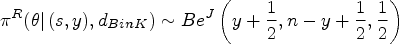
In other words, the naive $Be(\frac{1}{2},\frac{1}{2})$ prior is replaced by the design-dependent $B{e}^J(\frac{1}{2},\frac{1}{2},\frac{1}{2})$ prior to derive the posterior distribution. It is worthwhile noting that this posterior benefits from the status of objectivity based on the reference prior theory. However, in what follows we keep the name design-dependent Jeffreys interval that we note $C{I}^{ddJ}$ , and not design-dependent reference interval, because of the wide use of the first appellation. To figure out the influence of the $B{e}^J(\frac{1}{2},\frac{1}{2},\frac{1}{2})$ prior on the interval limits, Figure 2 displays the curves of the posterior densities for the observation $(s,y)=(1,5)$ obtained with $n=10$ in the design $d_{BinK0.5}$ with $K=2,3$ . It is clear that the mass of the design-dependent posterior density is shifted toward the continuation region on the $\theta$ scale (i.e. $\theta <0.5$ ) and the shift increases as $K$ increases.

Figure 2.

Naive (- - -) and design-dependent (—) posterior densities for the observation $(s,y)=(1,5)$ with $n=10$ in the design $d_{BinK0.5}$ with $K=2,3$ .

We now investigate the properties of the design-dependent Jeffreys interval. In the long-run frequentist context, the departure of the coverage probability from the confidence level is indicative of the influence of the stopping rule on the interval limits. Given the bivariate variable ( $S,Y$ ), the coverage probabilities of $C{I}_{low}$ and $C{I}_{upp}$ in the design $d_{BinK}$ are defined by

$$C_{low}(\theta ;d_{BinK})=P_{\theta }[\theta \ge {\hat{\theta }}_{low}(S,Y)]\text{ and }{C}_{upp}(\theta ;d_{BinK})=P_{\theta }[\theta \le {\hat{\theta }}_{upp}(S,Y)]$$

(18)

In what follows, the coverage of $C{I}^{ddJ}$ is compared to that of $C{I}^J$ and the frequentist alternative. The frequentist approach to interval estimation is based on the relation between hypothetical sequences $(k^{\prime },y_{k^{\prime }})>(k,y_k)$ ( $k,k^{\prime }=1,\dots ,K$ ). The interval limits are determined considering the probabilities of the hypothetical sequences beyond the observed one. Jennison and Turnbull ¹⁶ described a method based on the stage-wise ordering in which results corresponding to earlier termination are more extreme than those which terminate later. As for the Clopper–Pearson interval for fixed sample experiment, ³⁰ the Jennison-Turnbull interval ( $C{I}^{JT}$ ) is directly related to the binomial test as the interval limits result from the inversion of the $H_0$ acceptance zone.

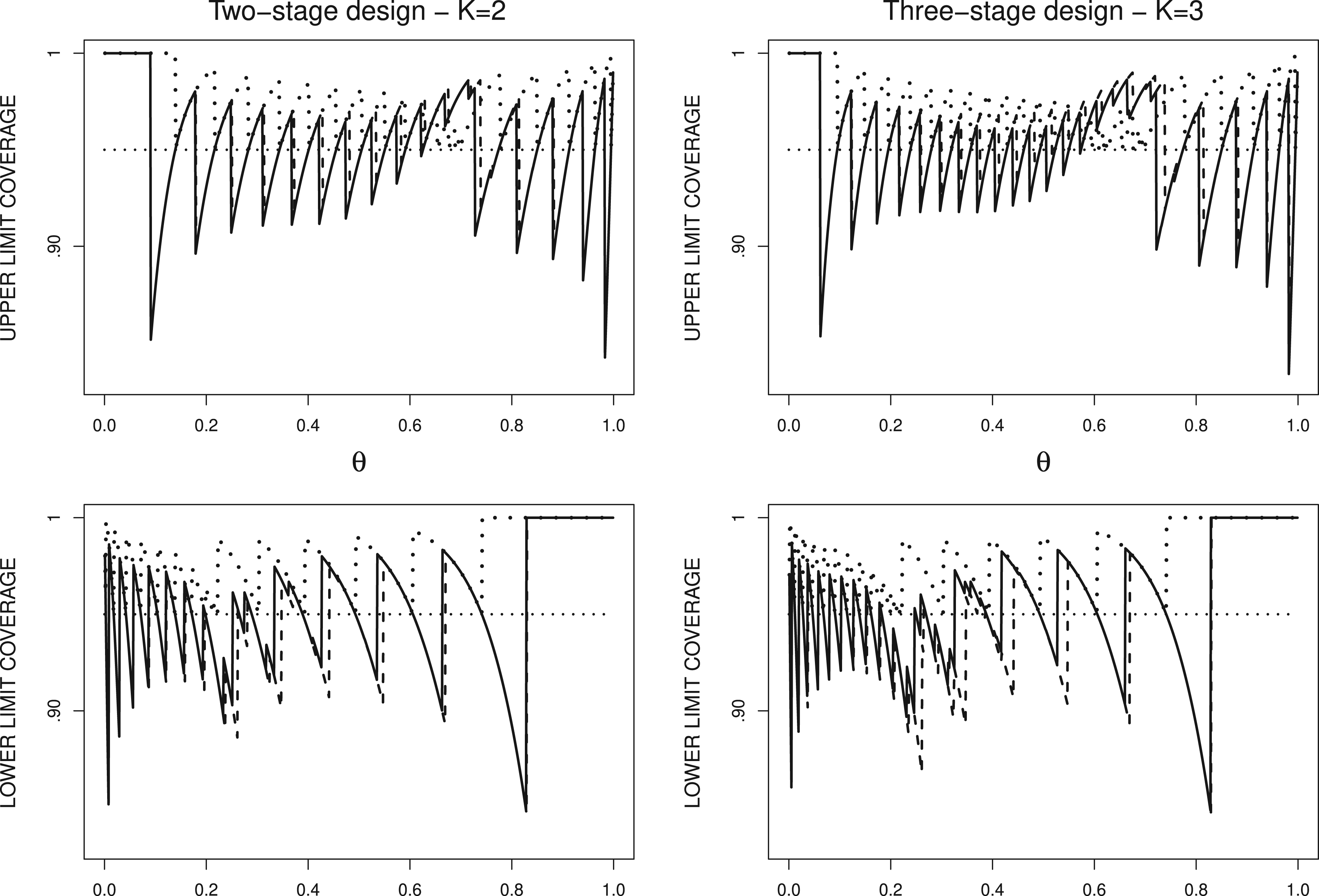
Figure 3 displays the one-sided coverage probabilities of $C{I}^J$ , $C{I}^{ddJ}$ , and $C{I}^{JT}$ with a confidence level of 95% in the design $d_{BinK0.5}$ with $K=2,3$ . The coverage curves contain non-negligible oscillations as $\theta$ varies that are caused by the lattice structure of the binomial distribution. The one-sided Jeffreys interval was studied in fixed sample experiment. ³¹ Using Edgeworth expansions, it is shown that the Jeffreys interval has no systematic bias in the coverage. However, the sequential nature of the experimental design implies another source of deviation. Figure 3 shows that the stopping rule causes an increase of the coverage probability of $C{I}_{upp}^J$ for the $\theta$ values around the upper interval limits for the observed rate $0.5$ (i.e. ${\hat{\theta }}_{upp}^J(1,5)=0.738$ , ${\hat{\theta }}_{upp}^J(2,10)=0.676$ , and ${\hat{\theta }}_{upp}^J(3,15)=0.646$ ) and a decrease of the coverage of $C{I}_{low}^J$ for the values of $\theta$ around the lower interval limits (i.e. ${\hat{\theta }}_{low}^J(1,5)=0.262$ , ${\hat{\theta }}_{low}^J(2,10)=0.324$ , and ${\hat{\theta }}_{low}^J(3,15)=0.354$ ). One can also observe that the influence of the stopping rule is partially corrected in the design-dependent Jeffreys interval, which exhibits lower magnitude of the spikes in the coverage probability curve. On another side, the Jennisson–Turnbull interval guarantees coverage probability of at least $1-\alpha$ by construction but the actual probabilities are far above the confidence level.

Figure 3.

One-sided coverage probabilities of the naive (- - -) and the design-dependent (—) Jeffreys intervals and the Jennison–Turnbull interval ( $\cdots$ ) with a confidence level of 95% in the design $d_{BinK0.5}$ with $K=2,3$ .

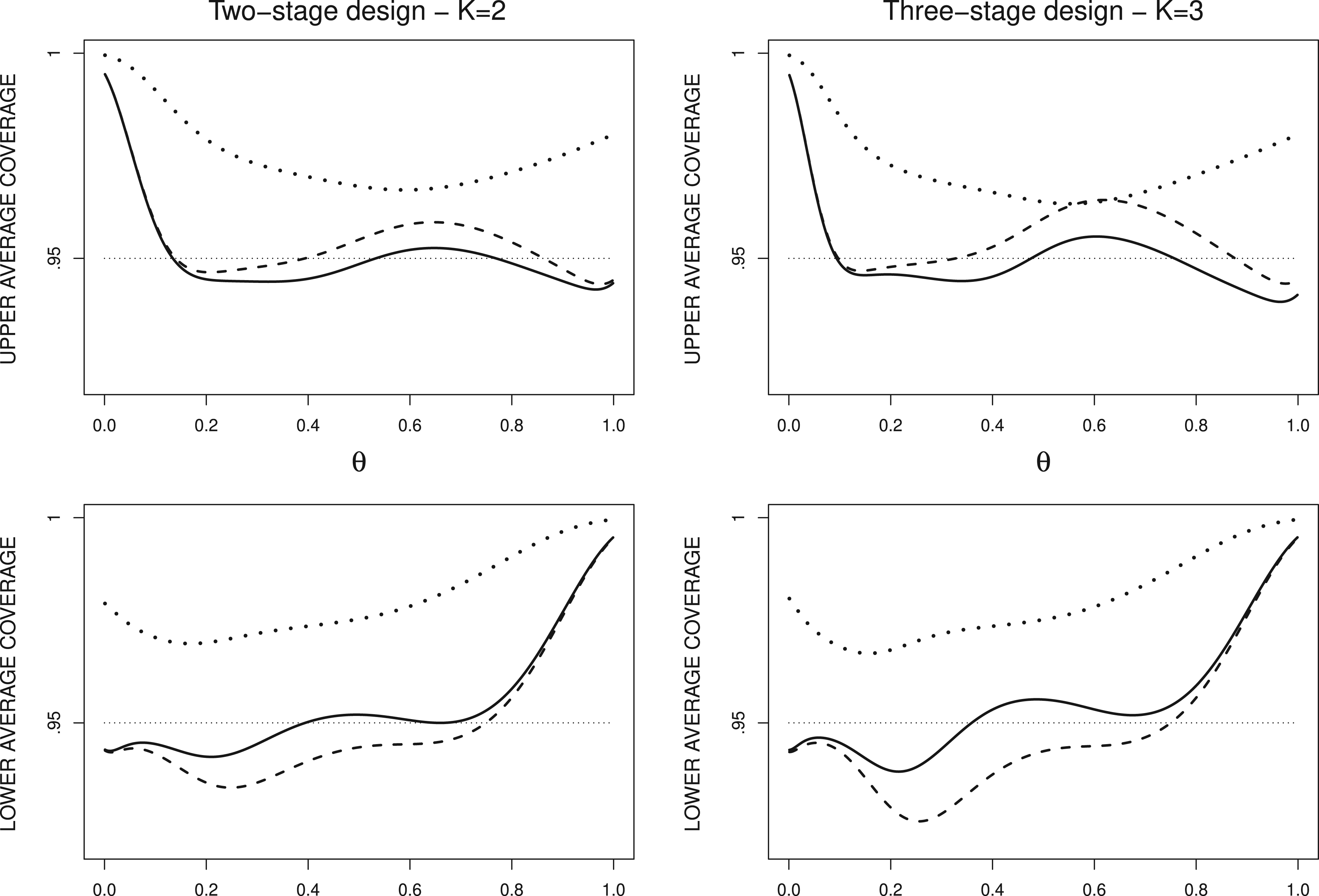
Due to the oscillation, the influence of the stopping rule on the coverage probability of $C{I}^J$ and the effect of the prior correction in $C{I}^{ddJ}$ are difficult to be interpreted in Figure 3. To overcome this, I propose a method which resumes some aspects developed for the average bias in the previous section. The variable ${\vartheta }_r$ defined in (15) allows the introduction of an amount of uncertainty around $\theta$ in function of the expected sample size in the experimental design. Now, let us integrate the coverage probabilities in (18) over the ${\vartheta }_r$ values with respect to its distribution, and consider the so-called one-sided average coverage probabilities which are defined as

$$\begin{array}{rl}A{C}_{low}(\theta ;d_{BinK})& ={\int }_{\mathrm{\Theta }}{P}_{{\theta }_r}[\theta \ge {\hat{\theta }}_{low}(S,Y)]dF({\theta }_r)\\ \text{ and }A{C}_{upp}(\theta ;d_{BinK})& ={\int }_{\mathrm{\Theta }}{P}_{{\theta }_r}[\theta \le {\hat{\theta }}_{upp}(S,Y)]dF({\theta }_r)\end{array}$$

(19)

The average coverage probability is the probability averaged over the values of ${\vartheta }_r$ that the confidence interval contains $\theta$ . Using Fubini’s theorem to interchange the order of integration in a double integral, it is easy to show that the average coverage probabilities considering ${\theta }_r$ and not $\theta$ (i.e. $\theta$ is replaced by ${\theta }_r$ in (19)) equal the coverage probabilities in (18).

Figure 4 displays the curves of the one-sided average coverage probabilities for $C{I}^J$ , $C{I}^{ddJ}$ , and $C{I}^{JT}$ with a confidence level of $95\mathrm{\%}$ in the design $d_{BinK0.5}$ with $K=2,3$ . The high average coverage of intervals at the extreme values of $\theta$ is caused by the zones of complete coverage, as shown in Figure 3, before the first spike for $C{I}_{upp}$ and after the last spike for $C{I}_{low}$ . This phenomenon decreases as the sample size increases. It is now clear that the design-dependent Jeffreys interval allows a lower departure of the average coverage probability from $1-\alpha$ than the (naive) Jeffreys interval. This departure is stronger for the values of $\theta$ around the interval limits for the observed rate $0.5$ . If we focus on the $\theta$ values in the range $(0.2,0.8)$ (excluding the zones of complete coverage), the maximum departure of $C{I}_{upp}^J$ is reached at $\theta =0.647$ in the two-stage design and is advanced to $\theta =0.619$ in the three-stage design, while the maximum departure of $C{I}_{low}^J$ is reached at $\theta =0.249$ in the two-stage design and is moved forward to $\theta =0.257$ in the three-stage design. The correction for the influence of the stopping rule in $C{I}^{ddJ}$ , as measured with the raw difference in the average coverage probabilities versus $C{I}^J$ , is stronger near the maximum departure of the average coverage probability of $C{I}^J$ . The maximum correction in $C{I}_{upp}^{ddJ}$ is reached at $\theta =0.635$ with $K=2$ and $\theta =0.705$ with $K=3$ and at $\theta =0.354$ with $K=2$ and $\theta =0.347$ with $K=3$ in $C{I}_{low}^{ddJ}$ . Regarding the Jennison–Turnbull interval, the average coverage probabilities are far above $0.95$ .

Figure 4.

One-sided average coverage probabilities of the naive (- - -) and the design-dependent (—) Jeffreys intervals and the Jennison–Turnbull interval ( $\cdots$ ) with a confidence level of $95\mathrm{\%}$ in the design $d_{BinK0.5}$ with $K=2,3$ .

This investigation confirms the good frequentist characteristics of the design-dependent Jeffreys interval. It also highlights the relevancy of the average coverage probability as a criterion to appraise the coverage properties of the confidence intervals in group sequential experiment. Section 2 of the appendix in Supplemental Material describes results of simulations to assess the effect of the prior correction on the average coverage of the two-stage design $d_{BinK0.5}$ with sample size increasing from $(n_1,n_2)=(10,10)$ to $(n_1,n_2)=(20,20)$ , $(n_1,n_2)=(50,50)$ , and $(n_1,n_2)=(100,100)$ . The results show that the effect of the prior correction on the design-dependent Jeffreys interval is proportional to the influence of the stopping rule on the naive Jeffreys interval as the sample size varies.

4. Comparison of the estimation approaches in three clinical trial designs

I now study the influence of the stopping rule and the effect of the prior correction on the point and the interval estimates through three classical two-stage designs in oncology clinical trials to test the rate of response to a therapeutic intervention. The parameters of the designs allow testing the one-sided hypotheses $H_0:\{\theta =0.2\}$ versus $H_1:\{\theta =0.4\}$ with the frequentist risks $\alpha =0.05$ and $\beta =0.20$ . The three designs are described hereafter:

In the Simon design, the trial stops early for futility (i.e. $H_0$ is accepted) at the interim analysis if the results are not promising. The minimax Simon design minimizes the maximum number of patients among the admissible Simon designs. This design requires the sample size $(n_1,n_2)=(18,15)$ .

The Pocock design allows an early stopping for efficacy (i.e. $H_0$ is rejected) using an aggressive stopping strategy since it applies a constant boundary on the $p$ -value scale at stage 1 and stage 2. The number of patients at stage 1 and stage 2 is set equal so that the sample size is $(n_1,n_2)=(21,21)$ .

The O’Brien–Fleming design combines early stopping for futility and efficacy. In our example, the sample size $(n_1,n_2)=(18,15)$ is the same as in the Pocock design, but the probability to reject $H_0$ at stage 1 is lower and greater at stage 2.

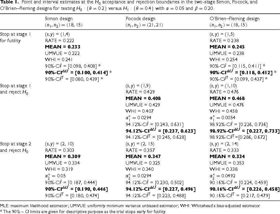
Table 1 gives the estimates obtained using the different approaches at the boundaries to accept and reject $H_0$ at stage $1$ and stage $2$ for the three experimental designs. Among the Bayesian point estimators, $MEAN$ is preferred to $MODE$ , which is not considered anymore in what follows, as the use of the posterior mean is more in accordance with the Bayesian practice than the posterior mode which mimics the methods based on likelihood maximization. Anyway, the estimates given by both Bayesian point estimators are very close. So, $MEAN$ is compared to $MLE$ , $UMVUE$ , and $WHI$ . Table 1 also shows the limits of the two-sided equal-tailed ( $1-2{\alpha }^{*})-CIs$ (or equivalently the limits of the one-sided ( $1-{\alpha }^{*})-CIs$ ) where the ${\alpha }^{*}$ value is the significance level of the one-sided test used to reject $H_0$ at each stage. In this manner, the confidence level of the intervals matches with the significance level of the tests. The limits of the design-dependent Jeffreys interval are compared to those of the (naive) Jeffreys interval and the Jennisson–Turnbull interval. Of note, in the Simon and the O’Brien–Fleming designs, the $90\mathrm{\%}-CI$ limits at the $H_0$ acceptance boundaries are given for descriptive purpose.

Table 1.

Point and interval estimates at the $H_0$ acceptance and rejection boundaries in the two-stage Simon, Pocock, and O’Brien–Fleming designs for testing $H_0:\{\theta =0.2\}$ versus $H_1:\{\theta =0.4\}$ with $\alpha =0.05$ and $\beta =0.20$ .

	Simon design	Pocock design	O’Brien–Fleming design
	$(n_1,n_2)=(18,15)$	$(n_1,n_2)=(21,21)$	$(n_1,n_2)=(18,15)$
Stop at stage 1	( $s,y$ ) = (1,4)		( $s,y$ ) = (1,5)
for futility	RATE = 0.222		RATE = 0.238
	MEAN = 0.233		MEAN = 0.245
	UMVUE = 0.222		UMVUE = 0.238
	WHI = 0.241		WHI = 0.254
	90%-CI J = [0.098, 0.408] *		90%-CI J = [0.115, 0.411] *
	90%-CI ddJ = [0.100, 0.414] *		90%-CI ddJ = [0.118, 0.412] *
	90%-CI JT = [0.080, 0.439] *		90%-CI JT = [0.099, 0.437] *
Stop at stage 1		( $s,y$ ) = (1,9)	( $s,y$ ) = (1,10)
and reject $H_0$		RATE = 0.429	RATE = 0.476
		MEAN = 0.408	MEAN = 0.468
		UMVUE = 0.429	UMVUE = 0.476
		WHI = 0.407	WHI = 0.458
		${\alpha }_1^{*}=0.0294$	${\alpha }_1^{*}=0.0054$
		94.12%-CI J = [0.243, 0.631]	98.92%-CI J = [0.226, 0.736]
		94.12%-CI ddJ = [0.237, 0.623]	98.92%-CI ddJ = [0.227, 0.733]
		94.12%-CI JT = [0.245, 0.628]	98.92%-CI JT = [0.286, 0.672]
Stop at stage 2	( $s,y$ ) = (2, 10)	( $s,y$ ) = (2, 15)	( $s,y$ ) = (2, 14)
and reject $H_0$	RATE = 0.303	RATE = 0.357	RATE = 0.333
	MEAN = 0.309	MEAN = 0.347	MEAN = 0.334
	UMVUE = 0.334	UMVUE = 0.325	UMVUE = 0.353
	WHI = 0.319	WHI = 0.340	WHI = 0.338
	${\alpha }_2^{*}=0.05$	${\alpha }_2^{*}=0.0294$	${\alpha }_2^{*}=0.0492$
	90%-CI J = [0.187, 0.444]	94.12%-CI J = [0.230, 0.502]	90.16%-CI J = [0.224, 0.459]
	90%-CI ddJ = [0.190, 0.446]	94.12%-CI ddJ = [0.227, 0.496]	90.16%-CI ddJ = [0.226, 0.458]
	90%-CI JT = [0.180, 0.474]	94.12%-CI JT = [0.223, 0.488]	90.16%-CI JT = [0.217, 0.479]

MLE: maximum likelihood estimator; UMVUE: uniformly minimum variance unbiased estimator; WHI: Whitehead’s bias-adjusted estimator.

* The $90\mathrm{\%}-CI$ limits are given for descriptive purpose as the trial stops early for futility.

In the Bayesian approach, the prior correction causes a shift of the posterior density mass toward the region of the experiment continuation to stage 2 on the $\theta$ scale. It is so expected that the prior correction results to an increase of the estimates in the Simon design and a decrease in the Pocock design. In the O’Brien–Fleming design, the continuation region is between the futility and the efficacy stopping boundaries at stage 1. If the observed rate is in, or close to, the continuation region, the posterior density mass will be more concentrated on its central value with the consequence that the design-dependent posterior mean will be close to that of the naive approach while the length of the credible interval will be reduced. Another consequence is that the effect of the prior correction on the posterior estimates is lower in the O’Brien–Fleming design than the Pocock design.

The correction for the influence of the stopping rule differs markedly according to the approach used. For point estimation, $WHI$ estimate is obtained from the $ML$ estimate ${\hat{\theta }}_{(s,y)}^{ML}$ by subtracting an estimate of the bias of the $MLE$ at $\theta ={\hat{\theta }}_{(s,y)}^{ML}$ . The correction is a function of ${\hat{\theta }}_{(s,y)}^{ML}$ only and applies equally whatever the stage number (i.e. without consideration for the actual sample size). Conversely, $UMVU$ estimate equals $ML$ estimate at stage 1 and the correction for the stopping rule bias applies at stage 2 only. For this reason the effect of the correction may appear counter intuitive as the statistical information is maximum at stage 2 and, in some cases, unduly strong. Unlike $UMVUE$ and $WHI$ , the correction for the influence of the stopping rule on $MEAN$ estimates takes into consideration the statistical information: The strength of the correction is inversely proportional to the observed sample size so that the correction is stronger at stage 1 than stage 2.

As for $UMVUE$ in point estimation, the correction on the limits of the Jennison–Turnbull interval applies at stage 2 only whereas the limits at stage 1 are those of the Clopper–Pearson interval in fixed $n_1$ -sample experiment. The main problem with the Jennison–Turnbull interval is that the limits are conservative due to great interval length. The reason is that this interval was developed with consideration for the preservation of coverage probability. The Jennison–Turnbull interval is usually not a good choice for practical use, unless strict adherence to the prescription that the one-sided coverage is at least $1-{\alpha }^{*}$ is required. In this setting, the design-dependent Jeffreys interval is an appealing alternative since the effect of the prior correction on the limits depends on the statistical information and the interval length is close to that of the naive Jeffreys interval. As previously mentioned, this credible interval also benefits from the objectivity of an approach which is strictly based on the reference prior theory.

This study of the correction for the influence of the stopping rule on the estimates highlights the relevancy of the full Bayesian strategy based on $MEAN$ for point estimation and the design-dependent Jeffreys interval for interval estimation.

5. Concluding remarks and discussion

The idea behind the reference prior theory is to maximize a distance between the prior and the posterior distributions, as data are collected. In return, the “data collected” have maximum influence on the posterior estimates. In sequential experiments, this interpretation can be extended to the “data collected in a given experimental design.” In the fixed sample binomial problem, the reference prior coincides with the prior obtained using Jeffreys’ criterion. The beta- $J$ distribution, which generalizes the reference prior distribution in sequential experiment, allows the development of a comprehensive and unified approach to the point and the interval estimations based on posterior estimators with good frequentist properties.

The comparative studies conducted in this article highlight the advantage of using the posterior mean based on the design-dependent Haldane prior in point estimation and the credible interval based on the design-dependent reference prior. The influence of the stopping rule on estimates is corrected depending on the available statistical information. The Bayesian approach provides estimates with coherent interpretation and allows avoiding the issues of pre-ordering in the observation space and non-unicity of the frequentist approach. The good properties of estimators were evidenced using the average bias in point estimation and the average coverage probability in interval estimation. These new criteria allow the introduction of an amount of uncertainty around the parameter value based on the preexperimental evidence given by the design.

Estimation of the binomial proportion upon sequential experiment termination is still a subject that arouses an abundant literature in the applied statistical community. ³² This article provides a Bayesian answer to address this issue. The objectivity status of the reference prior combined with the good frequentist properties of the posterior estimators, as well as the easiness of implementation using basic programming, justify to consider this comprehensive approach as one of the default choices in the experimental practice.

In sequential experiments with multiple binomial outcomes, it is natural to consider the use of multivariate binomial models with a dependence structure. However, it is often the case that only one or a subset of parameters is of interest, the others being nuisance parameters. The reference prior theory is particularly well adapted to this context as it allows a hierarchy among parameters. Let us consider the vector $\mathit{\theta }=({\theta }_1,{\theta }_2,\dots ,{\theta }_p)$ where there is a parameter, says ${\theta }_1$ , which is more of interest than the others, and suppose that the stopping rule depends on ${\theta }_1$ only. The design-dependent reference prior for this problem is the naive reference prior times the expected stopping time, ²¹ that is,

$${\pi }_{{\theta }_1}^R(\mathit{\theta }/d_K)\sim {\pi }_{{\theta }_1}^R(\mathit{\theta })E_{{\theta }_1}S$$

(20)

Whereas a Monte Carlo-type algorithm can be used to obtain the reference posterior summaries, the derivation of ${\pi }_{{\theta }_1}^R(\mathit{\theta })$ in (20) is a key aspect of the problem. To handle this, the reference prior theory allows a procedure which comes down to sequentially computing Jeffreys prior in one-parameter problem. ²⁵ This approach to nuisance parameter is based on an implicit ordering, for example, ( ${\theta }_1$ ,…, ${\theta }_p$ ). The reference prior relative to this ordering is obtained after successive conditioning (i.e. assuming each step that the conditional parameter is constant) such that:

$${\pi }_{{\theta }_1}^R(\mathit{\theta })={\pi }^R({\theta }_p|{\theta }_1,\dots ,{\theta }_{p-1})\cdots {\pi }^R({\theta }_2|{\theta }_1){\pi }^R({\theta }_1)$$

Supplemental Material

sj-pdf-1-smm-10.1177_09622802231199160 - Supplemental material for Bayesian estimation of the binomial parameter in sequential experiments

Supplemental material, sj-pdf-1-smm-10.1177_09622802231199160 for Bayesian estimation of the binomial parameter in sequential experiments by Pierre Bunouf in Statistical Methods in Medical Research