
Abstract
A frequently applied assumption in the analysis of data from cluster randomised trials is that the outcomes from all participants within a cluster are equally correlated. That is, the intracluster correlation, which describes the degree of dependence between outcomes from participants in the same cluster, is the same for each pair of participants in a cluster. However, recent work has discussed the importance of allowing for this correlation to decay as the time between the measurement of participants in a cluster increases. Incorrect omission of such a decay can lead to under-powered studies, and confidence intervals for estimated treatment effects can be too narrow or too wide, depending on the characteristics of the design. When planning studies, researchers often rely on previously reported analyses of trials to inform their choice of intracluster correlation. However, most reported analyses of clustered data do not incorporate a correlation decay. Thus, often all that is available are estimates of intracluster correlations obtained under the potentially incorrect assumption of no decay. In this article, we show that it is possible to use intracluster correlation values obtained from models that incorrectly omit a decay to inform plausible choices of decaying correlations. Our focus is on intracluster correlation estimates for continuous outcomes obtained by fitting linear mixed models with exchangeable or block-exchangeable correlation structures. We describe how plausible values for decaying correlations may be obtained given these estimated intracluster correlations. An online app is presented that allows users to obtain plausible values of the decay, which can be used at the trial planning stage to assess the sensitivity of sample size and power calculations to decaying correlation structures.
Keywords
Introduction
Longitudinal cluster randomised trials are cluster randomised trials where clusters are followed up over multiple trial periods. This class of designs includes parallel arm cluster randomised trials, stepped wedge trials, cluster randomised crossover trials, and associated variants such as incomplete stepped wedge designs. 1 Participants within clusters may provide data in one or more trial periods, although our focus is on the setting where each participant provides a single measurement, and we limit attention to a continuous outcome. When designing or analysing cluster randomised trials it is vitally important to account for the similarity between pairs of outcomes of participants in the same cluster. The simplest assumption is that the outcomes from participants in the same cluster are all equally correlated. In the stepped wedge literature, the model corresponding to this assumption is often referred to as the exchangeable model, or the Hussey and Hughes model. 2 However, more recently researchers have recognised the need to be able to allow for correlations between outcomes to vary based upon how far apart in time that they are measured. In many situations it is most reasonable to assume that outcomes recorded in the same time period will be more similar than those in differing time periods. There are two popular models for expressing this: the block-exchangeable model, where the correlation between a pair of participants in the same cluster only depends on whether they were measured in the same or different study periods3,4; and the discrete time decay model, which allows for the correlation between a pair of participants to decay exponentially as a function of the number of study periods between their recruitment. 5
When planning longitudinal cluster randomised trials, estimates of intracluster correlations and associated parameters are required for sample size/power calculations. 6 When the exchangeable model is assumed, researchers need only specify a single intracluster correlation, which describes the similarity in outcomes for participants in the same cluster regardless of time period. When the block exchangeable model is assumed, researchers must specify two parameters. The first is an intracluster correlation that describes the similarity of outcomes for participants in the same cluster recruited during the same time period (a within-period intracluster correlation). The second parameter is known as the cluster autocorrelation, which describes how this within-period intracluster correlation changes when a pair of participants in the same cluster but differing time periods is considered. When the discrete time decay model is assumed, values for the within-period intracluster correlation and cluster autocorrelation must once again be specified; however, the cluster autocorrelation now describes how the intracluster correlation changes when a pair of participants in the same cluster but adjacent periods is considered. We will refer to an intracluster correlation that quantifies the similarity of participants in a cluster regardless of timing of measurement (i.e. that assumed under the exchangeable model) as an aggregate intracluster correlation, so-called because rather than separating measurements into distinct trial periods, all measurements are aggregated together in the estimation of this intracluster correlation.
The discrete time decay model was introduced relatively recently. 5 The Shiny CRT app allows for the discrete time decay model in sample size calculations, 1 allowing researchers to input values for the intracluster correlation and the cluster autocorrelation. A repository of estimates of these discrete time decay model parameters was recently made available, 7 but to date there have been few longitudinal cluster randomised trials that have been designed assuming a discrete time decay correlation structure, and fewer still that have been analysed assuming this structure. The discrete time decay model can be fit in SAS, using the commercial ASReml-R package in R 8 ; it also appears that the free R package glmmTMB can be used to fit this model. 9 However, with the exception of the repository by Korevaar et al., 7 few estimates of the correlation parameters associated with the discrete time decay model are available; researchers may thus be unsure what values of these parameters are reasonable in their context.
In contrast, several repositories of aggregate intracluster correlation estimates, estimated assuming the exchangeable model, are available.10,11 Martin et al. 11 also included correlation parameter estimates for the block exchangeable model, while Korevaar et al. 7 included estimates for the exchangeable and block-exchangeable models for a bank of datasets. The exchangeable and block exchangeable models can be fit using any standard statistical software, for example using the free lme4 package in R, 12 in Stata, in SPSS, or in SAS, and estimates of the corresponding correlation parameters for individual trial outcomes are often available in published trial reports. An important question is whether the estimates of aggregate intracluster correlations that are available in such repositories and reports can tell us anything about plausible values of the parameters associated with a decaying correlation structure. That is, can we transform the estimates of intracluster correlation parameters obtained by fitting exchangeable or block exchangeable models to get estimates of the discrete time decay parameters? The answer is yes, such transformations are possible: using the expressions for estimated correlation components when an exchangeable or block exchangeable model have been incorrectly fitted instead of the discrete time decay model given by Kasza and Forbes, 13 we show how to obtain such transformed values. Such a transformation was previously applied by Kasza et al. 14 to obtain values of the discrete time decay cluster autocorrelation from published estimates of correlation parameters for the block exchangeable model. For an aggregate intracluster correlation obtained via the exchangeable model, a range of values of the discrete time decay correlation parameters will be consistent with this aggregate intracluster correlation.
In Section 2, we present the exchangeable, block exchangeable and discrete time decay models. In Section 3, we present the equations to be solved to transform correlation estimates obtained using the exchangeable or block exchangeable models to correlation estimates compatible with the discrete time decay model. We also include the equation for obtaining plausible values of the block exchangeable model's correlation parameters from the estimate of the intracluster correlation obtained from the exchangeable model. In Section 4, we apply the proposed method to two examples, demonstrating the use of our freely available online app (https://monash-biostat.shinyapps.io/ConsistentCACICC/). Using estimates by Korevaar et al., 7 in Section 5, we empirically evaluate our method by comparing the values for the cluster autocorrelation obtained using our method to those obtained when the discrete time decay model is directly fitted to a set of 16 datasets. In Section 6, we conclude with a short discussion.
The exchangeable, block exchangeable and discrete time decay models
We now present the three models that we will consider for continuous outcomes
Notation for the intracluster correlations, between-period intracluster correlations, and cluster autocorrelations for each of the three models considered.
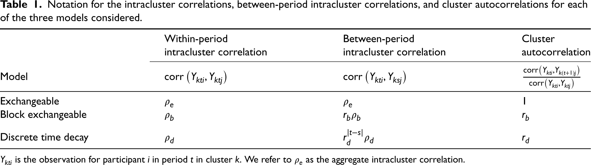
Notation for the intracluster correlations, between-period intracluster correlations, and cluster autocorrelations for each of the three models considered.
The three models we present in this section have previously appeared in the literature. For example, in the context of the stepped wedge design, the exchangeable model was originally presented by Hussey and Hughes,
2
the block exchangeable model was presented by Girling and Hemming
3
and Hooper et al.,
4
and the discrete time decay model was originally presented by Kasza et al.
5
For convenience, we present these models here.
The exchangeable model has the form:
The block exchangeable model (sometimes referred to as the nested exchangeable model
15
) has the form:
The discrete time decay model has the form:
This model includes a random effect for cluster, 
In addition to the random effect for cluster, 

We now consider three different scenarios. In the first scenario, estimates are available from the block exchangeable model, and need to be applied to a planned design under a discrete time decay model. In the second scenario, an estimate of the aggregate intracluster correlation is available from an exchangeable model and needs to be applied to a planned design under a discrete time decay model. Third, we provide a method for obtaining estimates for the block exchangeable correlation parameters from an estimate of the aggregate intracluster correlation.
We note that these methods apply to any type of longitudinal cluster randomised trial, including but not limited to the cluster crossover and stepped wedge designs. These results extend the work that was presented by Kasza and Forbes, 13 where the focus was on the impact of misspecification of the within-cluster correlation structure on inference for the treatment effect. Here we use the equations presented in that previous paper in a novel way to obtain values of correlation parameters associated with the discrete time decay and block exchangeable models that would have led to the observed exchangeable or block exchangeable correlation estimates. These conversion formulas have not been published previously. The derivation of results for our proposed approach is provided in the Supplemental Material.
When estimates are available from the block exchangeable model
If the block exchangeable model has been fit to clustered data, estimates of the within-period intracluster correlation
When estimates are available from the block exchangeable model, two equations with two unknowns must be solved. Hence, unique values for 
This equation states that the estimated cluster autocorrelation for the block exchangeable model is the average of all values of the within-cluster correlation matrix of cluster-period means, divided by 

The situation is more complicated when an estimate of the aggregate intracluster correlation is obtained from the exchangeable model: as we show in the Supplemental Material, there is now a single equation in two unknown parameters (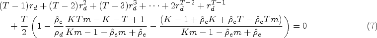
Alternatively,
In addition to the above, we propose an approximation to equation (7) which can be used when K and m are unknown:

We also consider the situation when researchers wish to obtain estimates of the block exchangeable correlation parameters from an estimate of the aggregate intracluster correlation. As was the case for obtaining estimates for discrete time decay correlation parameters from an estimate of the aggregate intracluster correlation, there is a single equation in two unknowns that must be solved. If 
Application to the diabetes data of Martin et al. 11
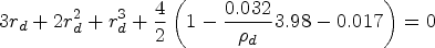
Martin et al. 11 provided a repository of intracluster correlations for the exchangeable and block exchangeable models for data from The Health Improvement Network (THIN) database. A range of outcomes from patients aged 18 years or over with a type-2 diabetes diagnosis, treated in one of 430 general practices in the United Kingdom were considered. Here we consider the HbA1c outcome, measured in patients between 1 January 2007 and 31 December 2007 (i.e. a period of 12 months). The estimated aggregate intracluster correlation for HbA1c over this 12-month period was 0.032. We assume 241 patients per practice in each 12-month period.
We suppose that interest is in planning a stepped wedge trial with periods of length three months each, and we wish to obtain values of the discrete time decay model intracluster correlation and cluster autocorrelation that are consistent with the value of 0.032 that was obtained by fitting the exchangeable model, although it is unlikely that period effects were included in this model. We assume minimal period effects here. The 12-month period that was used to calculate this intracluster correlation thus corresponds to 

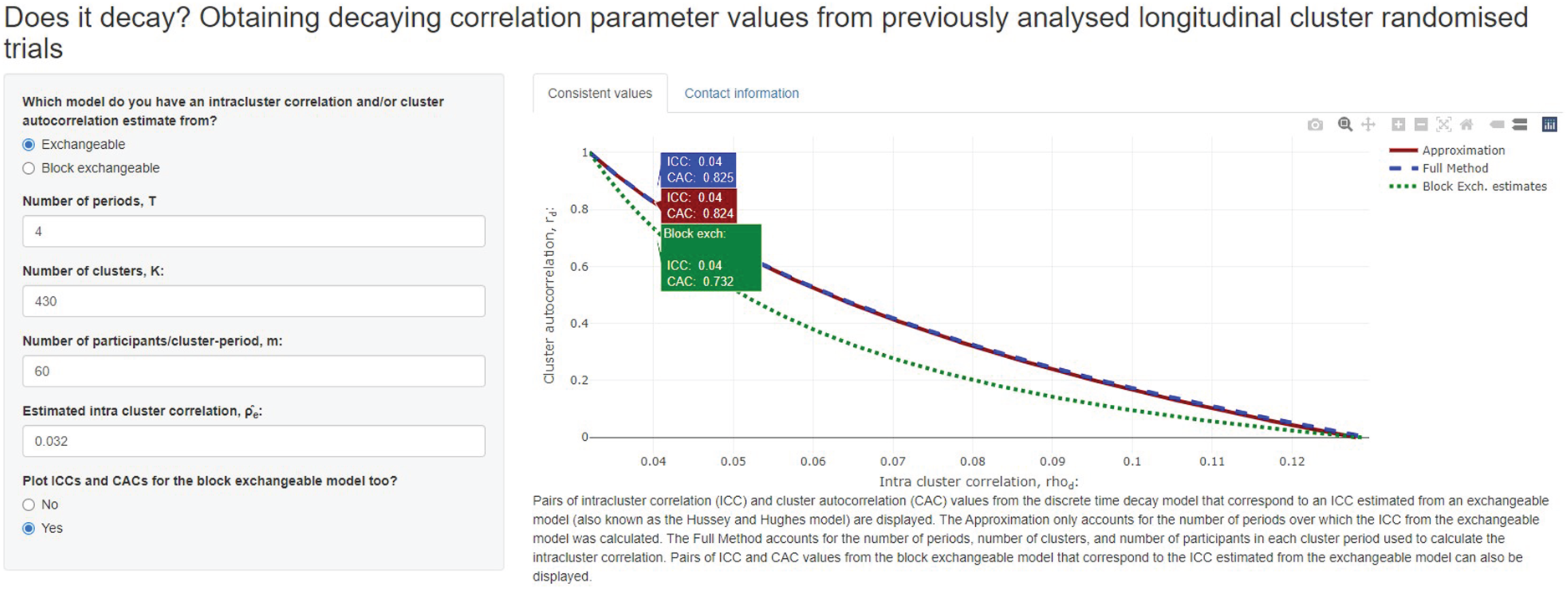
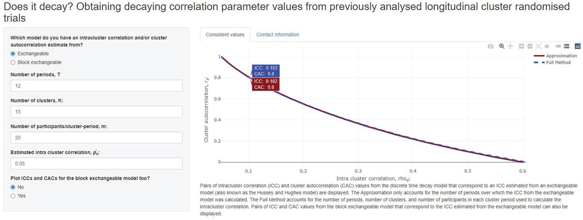
The pairs of intracluster correlation and cluster autocorrelation values that are aligned with the intracluster correlation obtained for the Hb1Ac outcome in. One particular set of values is highlighted:
The number of clusters required to be randomised to each sequence of a three-sequence stepped wedge design to detect a standardised effect size of 0.1 with 80% power and two-sided significance level of 0.05.
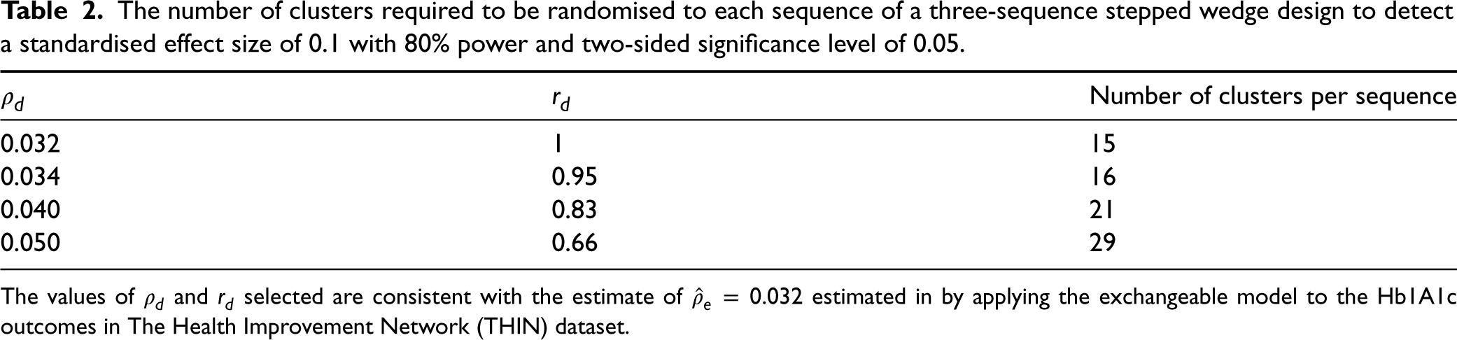
The values of
The range of plausible values can then be used to inform sample size and power calculations, with researchers considering the sensitivity of their calculations to various choices of
Acute atrial fibrillation (AF) and flutter (AFL) are common conditions seen in the Emergency Department (ED). In 2018, the Canadian Association of Emergency Physicians (CAEP) endorsed the acute AF/AFL best practices checklist which provides specific guidance for treatment in the ED. The RAFF-3 trial was a cross-sectional stepped-wedge cluster randomised design to evaluate implementation of the checklist at 11 large community and academic hospital EDs in Canada.
18
All 11 EDs started in the control condition (usual care). One hospital then crossed over to the intervention condition each month. There was a 2-month transition period to allow for implementation of the intervention. The primary outcome was length of stay in the ED in minutes from time of arrival to the documented time of discharge or hospital admission. The trial was designed to achieve at least 80% power to detect a 100-min reduction in ED length of stay, assuming an average of 10 patients per site per month, a standard deviation of 250 min, a within-period intracluster correlation of
To illustrate a more careful power calculation for the RAFF-3 trial, we consider routinely collected data on length of stay for a similar patient population obtained from 15 EDs with an average of 240 patients per ED over a period of one year. For privacy reasons, patient-level data could not be obtained but the aggregate intracluster correlation was provided as
The pairs of intracluster correlation and cluster autocorrelation values that are consistent with the intracluster correlation obtained for the length of ED stay in RAFF-3 trial. One particular set of values using full method is highlighted:
Using the Shiny CRT sample size calculator, we enter a stepped wedge cross-sectional design with 11-sequences, one cluster per sequence, a total duration of 14-months with a 2-month implementation period and 10 patients in each cluster-period, aiming to detect a standardised effect size of 0.4 with a two-sided significance level of 0.05. The power that can be achieved with the reasonable combinations of within-period intracluster correlation and cluster autocorrelations is shown in Table 3. If an exchangeable model were assumed, this design will achieve 96.2% power. However, if the plausible values under the discrete time decay model are considered, power will drop substantially using the same design and could be as low as 54.7%.
The power that can be achieved by the rapid atrial fibrillation and flutter 3 (RAFF-3) trial to detect a standardised effect size of 0.4 with two-sided significance level of 0.05.
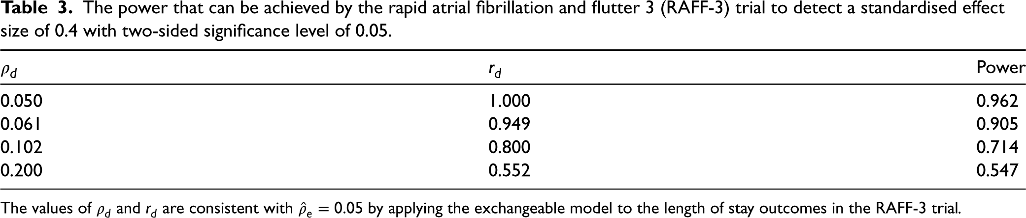
The values of
We demonstrate that the issue of the selection of a suitable within-cluster correlation structure and associated parameters is often much less problematic for parallel cluster randomised trials. We consider a parallel cluster randomised trial variant of the RAFF-3 stepped wedge, with five clusters randomised to each arm of a 12-period parallel cluster randomised trial, with 10 participants in each cluster in each period. Using the same set of correlation parameters as given in Table 3, we determined the power of this parallel variant of the RAFF-3 trial to detect an effect size of 0.4, with the results presented in Table 4. Although the power of the design does change depending on the correlation parameters, this example demonstrates that the parallel design is much less sensitive to the precise choice of correlation parameters than the stepped wedge design.
The power that can be achieved by a parallel variant of the rapid atrial fibrillation and flutter 3 (RAFF-3) trial to detect a standardised effect size of 0.4 with two-sided significance level of 0.05.
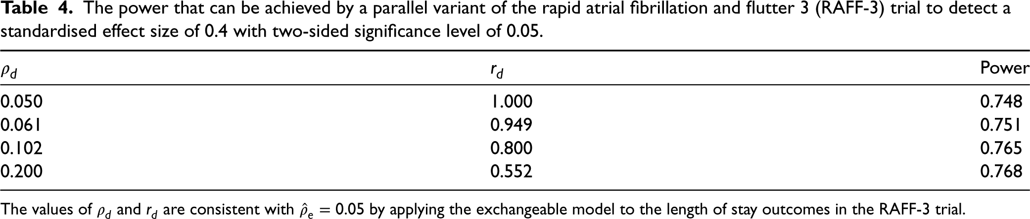
The values of
Estimated correlation parameters obtained for CLOUD Bank datasets, obtained by fitting the block exchangeable and discrete time decay models, and the discrete time decay cluster autocorrelation obtained by applying equation (6).
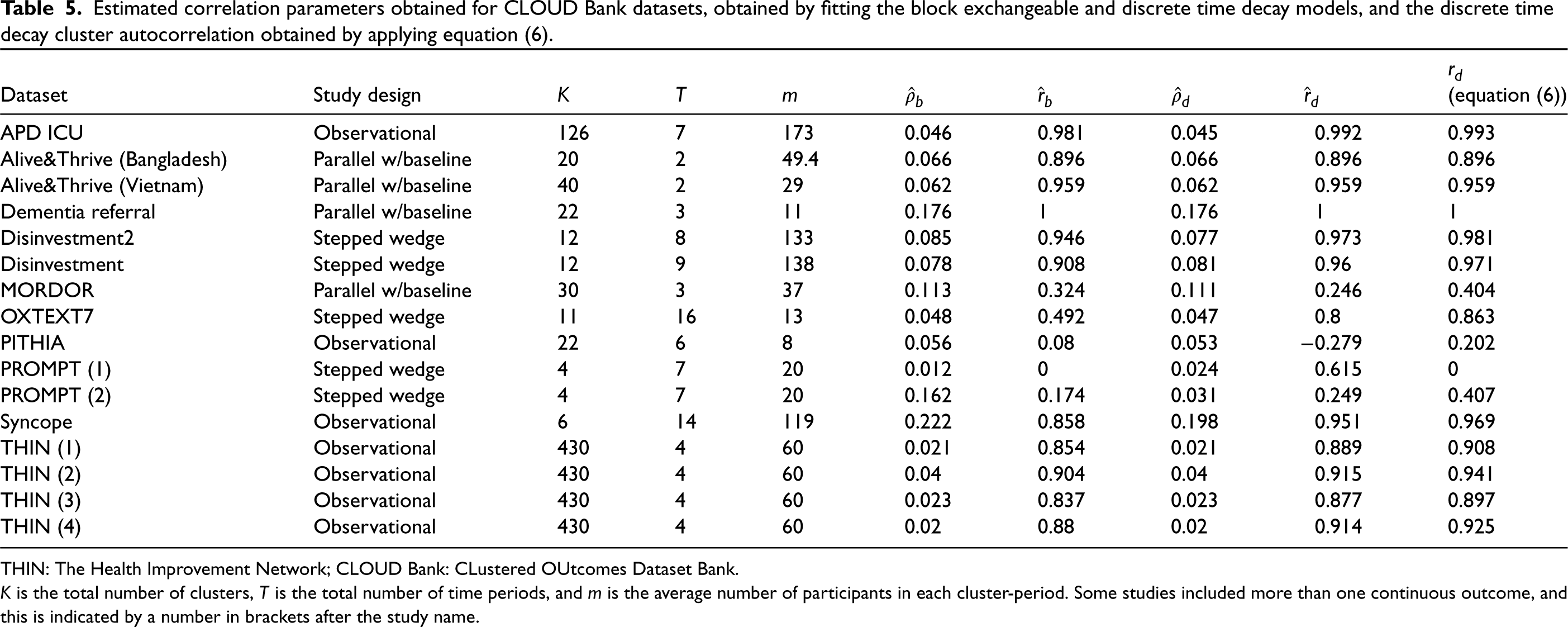
THIN: The Health Improvement Network; CLOUD Bank: CLustered OUtcomes Dataset Bank.
In Korevaar et al.,
7
several longitudinal clustered datasets (known as the CLustered OUtcomes Dataset Bank) were analysed using all three of the models presented in Section 2, and we consider the 12 studies where each participant provided only one measurement of each outcome during the course of the study. One study included two outcomes, and another included four, for a total of 16 datasets. The name of each study, the design of each study, the number of clusters (
Table 5 shows that the use of equation (6) resulted in similar estimates to those directly obtained by fitting the model when the model-based cluster autocorrelation was high (greater than around 0.85). Twelve of the 16 datasets had estimates of
There were quite large differences between the model-based estimate of
Discussion
In this article, we have described an approach for obtaining plausible values of the correlation parameters associated with the discrete time decay when correlation parameter estimates are available from the exchangeable or block exchangeable model; and for obtaining plausible values for the correlation parameters associated with the block exchangeable model when correlation parameter estimates are available from the exchangeable model. These methods assume that the estimates of the parameters from the exchangeable or block exchangeable model have come from a balanced dataset: the same number of participants has provided data in all clusters in all periods, and each participant has only provided data in one period. Hence, these methods should not replace the actual estimation of the model parameters in R or SAS: if raw data are available to be analysed, these data should be analysed to provide estimates of the within-period intracluster correlation and cluster autocorrelation for the discrete time decay or block exchangeable model. Further, the methods we have presented assume that a linear mixed model for outcomes is appropriate, and thus their use for non-continuous outcomes may not be valid.
When planning a longitudinal CRT, researchers may inadvertently use an anticipated aggregate intracluster correlation in lieu of the within-period ICC in the sample size calculation procedure. However, this could lead to under-estimating the required sample size as the within-period ICC must be inflated to allow for the decaying cluster autocorrelation and is therefore necessarily larger than the aggregate ICC. That is,
Application of the method to the datasets in the CLOUD Bank indicates that there is often good agreement between the estimates of
The block exchangeable and discrete time decay models that we have presented depend on the notion of trial ‘periods’: trials are assumed to be split into time periods of equal length. For these models, the intracluster correlation and cluster autocorrelation depend on the length of these trial periods, and thus need to be recalculated when interest is in periods of differing lengths. Recent work has suggested that in certain circumstances it would be more appropriate to consider time as a continuous phenomenon in longitudinal cluster randomised trials, especially when recruitment of participants occurs continuously throughout each study period.20,21 A continuous time decay correlation structure that considers the precise times of measurement rather than the period of measurement in defining the correlations between pairs of observations was introduced by Grantham et al. 22
The methods that we have presented allow researchers to obtain some understanding of plausible values of the correlation parameters associated with the discrete time decay model, even when such a model has not been fit to the dataset. Although the paper introducing the discrete time decay model has been quite influential in the stepped wedge literature, 23 few longitudinal cluster randomised trials have yet been designed or analysed assuming a discrete time decay (with the exception of the secondary analyses of several studies that was presented by Korevaar et al. 7 ). Hence, when planning longitudinal cluster randomised trials, there are few estimates of the discrete time decay correlation parameters available for researchers to rely upon. The methods we have presented allow researchers to obtain plausible values to be used in sample size and power calculations, and have been implemented in an online app available at https://monash-biostat.shinyapps.io/ConsistentCACICC/.
Supplemental Material
sj-pdf-1-smm-10.1177_09622802231194753 - Supplemental material for Does it decay? Obtaining decaying correlation parameter values from previously analysed cluster randomised trials
Supplemental material, sj-pdf-1-smm-10.1177_09622802231194753 for Does it decay? Obtaining decaying correlation parameter values from previously analysed cluster randomised trials by Jessica Kasza, Rhys Bowden, Yongdong Ouyang, Monica Taljaard and Andrew B Forbes in Statistical Methods in Medical Research
Footnotes
Declaration of conflicting interests
The author(s) declared no potential conflicts of interest with respect to the research, authorship, and/or publication of this article.
Funding
The author(s) disclosed receipt of the following financial support for the research, authorship, and/or publication of this article: This work was supported by the National Health and Medical Research Council of Australia Project Grant ID 1108283.
Supplemental material
Supplemental material for this article is available online.
References
Supplementary Material
Please find the following supplemental material available below.
For Open Access articles published under a Creative Commons License, all supplemental material carries the same license as the article it is associated with.
For non-Open Access articles published, all supplemental material carries a non-exclusive license, and permission requests for re-use of supplemental material or any part of supplemental material shall be sent directly to the copyright owner as specified in the copyright notice associated with the article.