
Abstract
The zero-inflated negative binomial distribution has been widely used for count data analyses in various biomedical settings due to its capacity of modeling excess zeros and overdispersion. When there are correlated count variables, a bivariate model is essential for understanding their full distributional features. Examples include measuring correlation of two genes in sparse single-cell RNA sequencing data and modeling dental caries count indices on two different tooth surface types. For these purposes, we develop a richly parametrized bivariate zero-inflated negative binomial model that has a simple latent variable framework and eight free parameters with intuitive interpretations. In the scRNA-seq data example, the correlation is estimated after adjusting for the effects of dropout events represented by excess zeros. In the dental caries data, we analyze how the treatment with Xylitol lozenges affects the marginal mean and other patterns of response manifested in the two dental caries traits. An
Keywords
Introduction
Motivation
In biomedical research, count data often include a large number of zeros. For example, quite often people do not have dental caries, 1 and the majority of a population does not make a hospital visit during a given year. 2 In omics data, either because of technological reasons related to sequencing or due to some biological reasons, counts are often very sparse.4,5,3
Such count data with excess number of zeros are frequently modeled using the zero-inflated Poisson (ZIP) or the zero-inflated negative binomial (ZINB) distributions.7,6 The negative binomial distribution, of which the Poisson distribution is a limiting case, has a capacity of modeling overdispersion that accounts for the heterogeneity of the incidence processes and thus is widely used in practice. Zero-inflation refers to the phenomenon where the proportion of zeros is greater than is expected by the corresponding baseline distribution.
However, these univariate models only provide insights about marginal distributions and do not inform the joint characterization of two dependent count variables. For example, when the association of two genes is of interest, a bivariate model is needed to effectively estimate the dependence. On the other hand, in caries and other clinical trials, a joint model may be beneficial when univariate analyses are less efficient for comparing marginal mean outcomes between treatment groups. As in the choice of multivariate analysis of variance versus multiple analysis of variances for the hypothesis testing of continuous random variables, multivariate count models can control type-I error in a more efficient way than multiple testing based on univariate ZIP or ZINB models. 8 To meet these different purposes, we develop a flexible bivariate ZINB model that characterizes the joint distribution of two correlated count random variables.
The two motivating examples are used to illustrate the utility of the proposed bivariate model for count data in biomedical research. The first one involves the estimation of dependence of two genes in single-cell RNA sequencing (scRNA-seq) data that have a significant amount of dropouts, which are represented by excess zeros under model assumptions. The pairwise dependencies are important as they serve as building blocks for identifying pathways. However, possible dropout events obfuscate measuring the dependence of gene pairs in the absence of dropout. For this task, we estimate the dependence after controlling for the dropout events through a bivariate zero-inflation model. The second example is characterizing the distribution of the number of dental caries detected on two different tooth surfaces. A treatment—Xylitol lozenges—may not only affect the mean count for both traits to varying degrees but also may modify the structure of the joint distribution. A bivariate model is needed to adequately characterize the joint distribution and estimate marginal effects on outcomes with possibly improved precision. More details of the two examples are given in the following subsections.
Measuring genewise dependence in scRNA-seq data
Single-cell RNA sequencing (scRNA-seq) is a high throughput sequencing technology that profiles gene expression at a cell’s resolution. 9 This is in contrast to bulk RNA sequencing (RNA-seq), where a group of cells are sequenced altogether and consequently, no cell-level information is available in data. As a price for cell-level resolution, scRNA-seq loses some information by the so-called “dropout” phenomenon; during the sequencing steps (and the capturing steps, e.g. in 10X sequencing platform) of scRNA-seq, a large amount of RNAs are undetected. Consequently, the observed count data include a greater number of zeros than would be expected given the number of molecules sequenced and our a priori knowledge of transcription rates at individual loci.4,10,11 In contrast, in a bulk RNA-seq, excess zeros are less frequently observed. 10 For these reasons, negative binomial models have been extensively used for bulk RNA-seq data,12,14,13 and ZINB models are typically used for scRNA-seq data.5,4 Although recent technologies such as unique molecular identifiers (UMIs) effectively remove the dropout events, the problem still persists in data obtained from many of the non-UMI-based platforms.
Statistical inferences at both individual gene level15,16 and gene set level, for example, pathways, can be misleading without considering the excess zeros caused by dropouts. Inference of gene-gene dependence, for example, the correlation-based method, has been widely used in pathway analysis of bulk RNA-seq data 17 and in recent scRNAseq data analyses.15,16,19,20,18 However, the conventional Pearson correlation of two genes with significant dropouts in the scRNAseq may not properly reflect the underlying gene-gene dependence.
For example, a pair of genes, of which expressions are highly correlated with the absence of dropouts, would have an attenuated correlation, based on the observed data, if only one of the genes have a large amount of dropouts. On the other hand, a pair of uncorrelated genes would have a higher correlation, when both genes have dropouts in a substantial portion of the sample. The systematic bias will not vanish without adjusting for the effects of the dropout events, regardless of the dependence measure such as Pearson correlation and mutual information.
Two strategies have been considered to address the bias in scRNA-seq data. Imputation methods21,18,22 aim to provide expression levels free of the excess zeros by imputing them. While imputation methods are versatile in that they provide ready-to-use data, they are not deterministic, having different results for every implementation, and analyses results over multiple imputations may have to be combined. The other strategy is an estimation of the count distribution.11,23 Once having obtained information about the distribution of the expressions before dropouts, one can do downstream analyses such as measuring the dependence of the before-dropout expressions. However, many of the methods taking this approach focus on modeling marginal distributions and they do not explicitly posit dependence structure between two genes.
Our proposed method, to be introduced in Section 1.4, takes the distribution estimation approach where a bivariate distribution explicitly addresses the dependence structure. Specifically, our method is built on a bivariate generalization of the ZINB model, where the dropout probabilities are modeled using the zero-inflation parameters. In this approach, the full joint distribution is estimated using a bivariate count model with zero-inflation and the underlying distribution before dropouts is uncovered to estimate the dependence.
Characterizing the joint count distribution of two dental caries traits
The second example is about describing the pattern of the number of dental caries occurring at two different tooth surface types in a randomized clinical trial (the Xylitol for Adult Caries Trial, or X-ACT).
24
In one of its secondary studies, the effect of Xylitol lozenges on the incidence of three different dental caries outcomes were examined with univariate models according to the type of tooth surface: smooth-surface caries, proximal-surface caries, and occlusal-surface caries.
25
To be more specific, we refer to dental caries as the annualized D
However, the original analysis can only tell us about the marginal distribution of each trait and does not provide any information of their joint structure. For example, Xylitol lozenges may have lowered the correlation between the proximal- and smooth-surface caries by reducing the concordant pairs (zero for both or non-zero for both) while increasing the discordant pairs (zero for one and non-zero for the other). A joint analysis may give additional clues for identifying the mechanism of Xylitol lozenges and can only be obtained through joint modeling of the traits. We analyze the joint distribution of a pair of traits using our bivariate extension of the ZINB distribution.
The bivariate models could also be used to boost statistical efficiency in marginal analyses, since the information contained in one variable could be borrowed in making inferences on the other. For instance, in testing the group difference of mean incidence rates on smooth surfaces, the joint incidence rate of smooth and proximal surfaces could be estimated with a bivariate model and the group differences could be tested for each margin at an enhanced precision.
Review of existing bivariate count models and the proposed method
In consideration of building bivariate count models, it is noteworthy that there have been proposed a variety of bivariate models that fit overdispersed count data: bivariate Poisson mixture models,28,27,29 bivariate generalized Poisson models, 30 and copula models.31,13,32 These models can be further extended to flexibly accommodate excess zeros by introducing zero-inflation parameters or composing hurdle models. For a comprehensive survey of bivariate count models, refer to Cameron and Trivedi 33 and Chou and Steenhard. 34
Of a plethora of the proposed models in the literature, many of the bivariate Poisson mixture models and bivariate generalized Poisson models take overly complicated forms, they do not have simple marginal distributions (e.g. GBIVARNB model by Gurmu and Elder 28 ), and their parameters are hard to interpret and/or computationally expensive to estimate. Copula-based bivariate models can be alternatives to the mixture models, but they depend on the underlying copula models and can be difficult to interpret.
Many existing bivariate negative binomial models are primarily designed for modeling marginal means rather than pairwise dependence. For example, Gurmu and Elder 28 discussed a bivariate negative binomial distribution (BIVARNB), but their model is specified by only four parameters, which may not provide sufficient flexibility to delineate diverse distributional structure. For such a bivariate joint distribution, four parameters are needed to specify the first two marginal moments of each of the two variables, while another parameter is needed solely for modeling the dependence. Subsequently, Wang 35 extended BIVARNB to a zero-inflated BIVARNB regression setting. In this model, zero-inflation is dictated by a single parameter, implying that when one variable either drops out or not, the other variable behaves exactly the same, which may not be the case for scRNA-seq data; one gene can drop out, while the other does not in a sample. Instead, it is possible to have three free parameters for the full joint zero-inflation probability structure. 36
We propose a bivariate zero-inflated negative binomial model with eight parameters: five parameters for the negative binomial part and another three free parameters for the zero-inflation part. This model allows analyzing the dependence of two zero-inflated count variables parametrically but with more flexibility than existing models. Specifically, five parameters of our proposed model characterize all moments of the first two orders before zero-inflation, and the three zero-inflation parameters model the dropouts or the membership of non-susceptible groups with full flexibility.
Besides the flexibility and the provision of the dependence measure, the proposed BZINB model has the following features. The parameters have simple latent variable interpretations, the joint distribution can be marginalized into the corresponding univariate ZINB distributions, and the model can be easily reduced to a non-zero-inflated model, or BNB, by dropping the zero-inflation parameters.
The rest of the article is organized as follows. In Section 2, we describe how the model is constructed based, successively, on a bivariate negative binomial (BNB) model and a bivariate ZINB (BZINB)model. We present the maximum likelihood estimator using the expectation-maximization (EM) algorithm in Section 3. In Section 4, we illustrate how well the model fits data and how the model-based dependence measure behaves in contrast to naive measures using mouse paneth scRNA-seq data and study the performance of the dependence measure via simulations. In Section 5, we analyze the dental caries clinical trial data with the BZINB model to characterize the joint distribution of two dental caries traits, and illustrate the use of the model in testing the group differences in the marginal means of the two traits. In Section 6, we address the limitations of the models and discuss potential extensions. Section 7. provides software information.
The model
A BNB model
In constructing the BZINB model, to induce dependence and zero-inflation, layers of latent variables were used as in Kocherlakota and Kocherlakota 37 and Li et al. 36 We first introduce a simpler model, the BNB model in this subsection, and then generalize it to the BZINB model in Section 2.2.
The key assumption that induces the dependence structure of BNB (and BZINB) is that the mean parameters of two Poisson random variables are sums of gamma random variables that share a common gamma random variable. Let

This BNB model is marginally negative binomial, as we know from the construction procedure that both
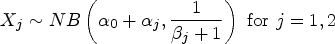
Interpretation of the BNB parameters is straightforward:
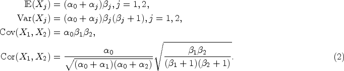
The first two moments and the correlation of a BNB random pair are given as
Maher 38 developed another bivariate negative binomial distribution that is a constrained case of BNB in a sense that the marginal means and variances are the same for both variables.
One can further generalize this BNB model into a
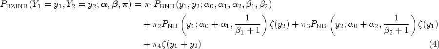
In this subsection, we generalize the BNB model to the BZINB model by including zero-inflation components. Since BZINB is also a generalization of the univariate ZINB model, we illustrate the construction of the univariate ZINB model first and move to the bivariate version.
A univariate negative binomial model,
Similarly, a multivariate zero-inflated random variable can be constructed using a latent variable that follows the multivariate Bernoulli distribution as in the Poisson case.
36
For a bivariate distribution, suppose we have a random vector

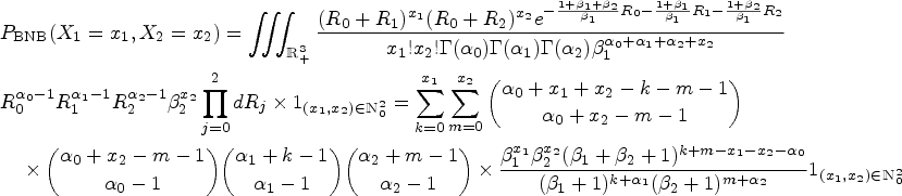
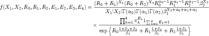
From the construction of the latent variables in the above paragraph, the probability mass function of a BZINB variable is derived as
Here, the parameters
In scRNA-seq data,
This BZINB distribution is marginally ZINB, since the latent random variables,


With the natural interpretation of the BZINB model as layers of latent variables, one can estimate the parameters by the expectation-maximization (EM) algorithm.
The joint probability density of the observed and latent variables (“complete likelihood”) is given as

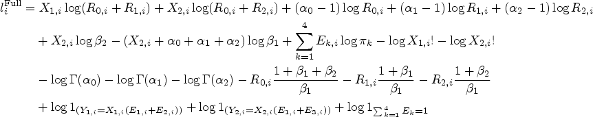
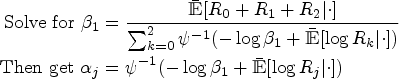
As the likelihood is the product of functions concave with respect to each of the parameters at the expectation (see Web Section B.2 of the Supplemental Materials), the maximization can be achieved by solving a system of score equations. The individual scores are given as
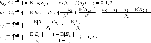
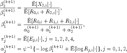
At the
The standard error of the maximum likelihood parameter estimates can be calculated using observed information. In Web Section D of the Supplemental Materials, detailed formulae are given, and simulations illustrating the accuracy of standard error estimation are included in Section 4.3.
Model comparison using the mouse paneth data
In this section, we show how the BZINB model fits a scRNA-seq data set compared to its nested models (in Section 4.1.), present how model-based dependence measures can be different from naive measures (in Section 4.2.), and study the asymptotic behavior of the estimator through simulations in Section 4.3. The data were collected from paneth cells of a C57Bl6 mouse with a Sox9 gene knockout. The Fluidigm C1 system was used to capture single cells and generate Illumina libraries using manufacturers’ protocols. Illumina NextSeq sequencing platform was used for paired-end sequencing. Reads per cell were demultiplexed using mRNASeqHT_demultiplex.pl, a script provided by Fluidigm. Low quality base calls and primers were removed using Trimmomatic 39 and poly-A tails were removed using a custom perl script. Reads were aligned to the mouse genome (mm9) using STAR (https://academic.oup.com/bioinformatics/article/29/1/15/272537) and read per gene were counted using htseq-count (https://www.ncbi.nlm.nih.gov/pmc/articles/PMC4287950).
The data are composed of 23,425 genes for 800 cells, where all the cells came from a single mouse and have the same cell type. Over 90% of genes have more than 90% zero counts and the average (minimum, 25th percentile, 75th percentile, and maximum) proportion of zero counts for a gene is 97.3% (4.8%, 97.0%, 99.9%, and 100%) in the data. We perform a zero-inflation test to detect zero inflation, since a high proportion of zeros may not necessarily mean zero inflation. The likelihood ratio test comparing the NB and ZINB distribution is used for this test with a 50:50 mixture
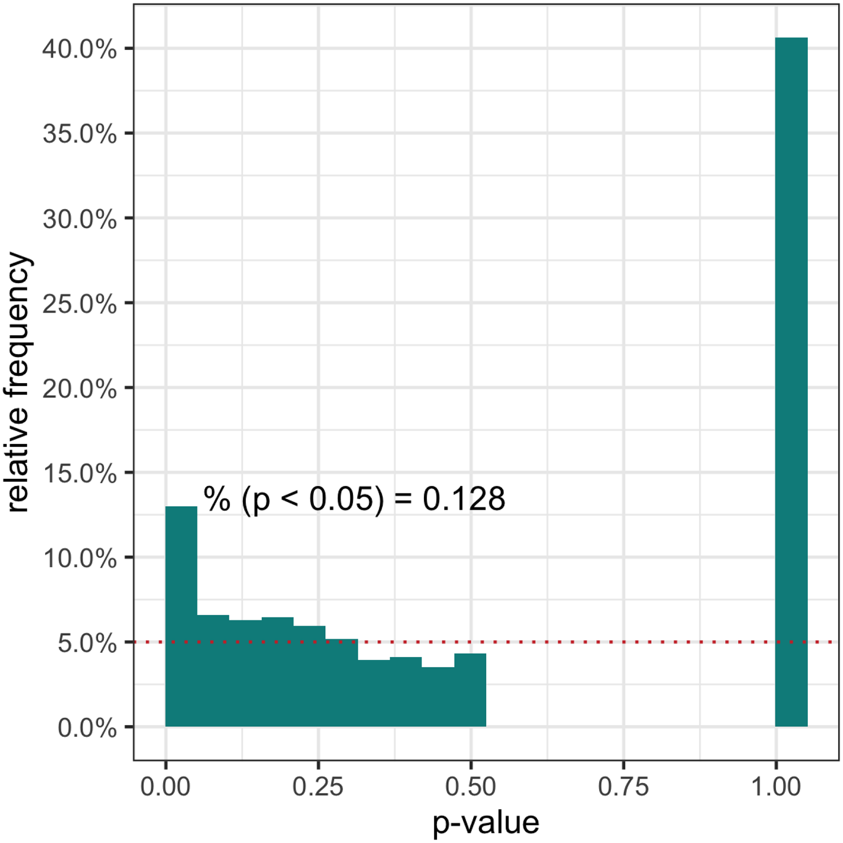
The histogram of the likelihood ratio test for zero-inflation. The reference
We compare four nested models: BZINB, BNB, bivariate zero-inflated Poisson (BZIP), and bivariate Poisson (BP). BZIP has fixed mean values instead of latent gamma variables of BZINB, and BP further lacks zero-inflation components. The estimated probability distribution of these models is compared with the empirical distribution of the 50 gene pairs.
To systematically study the model performances, we performed a stratified sampling of genes according to their proportion of zeros; strata H, M, L, and V include genes with
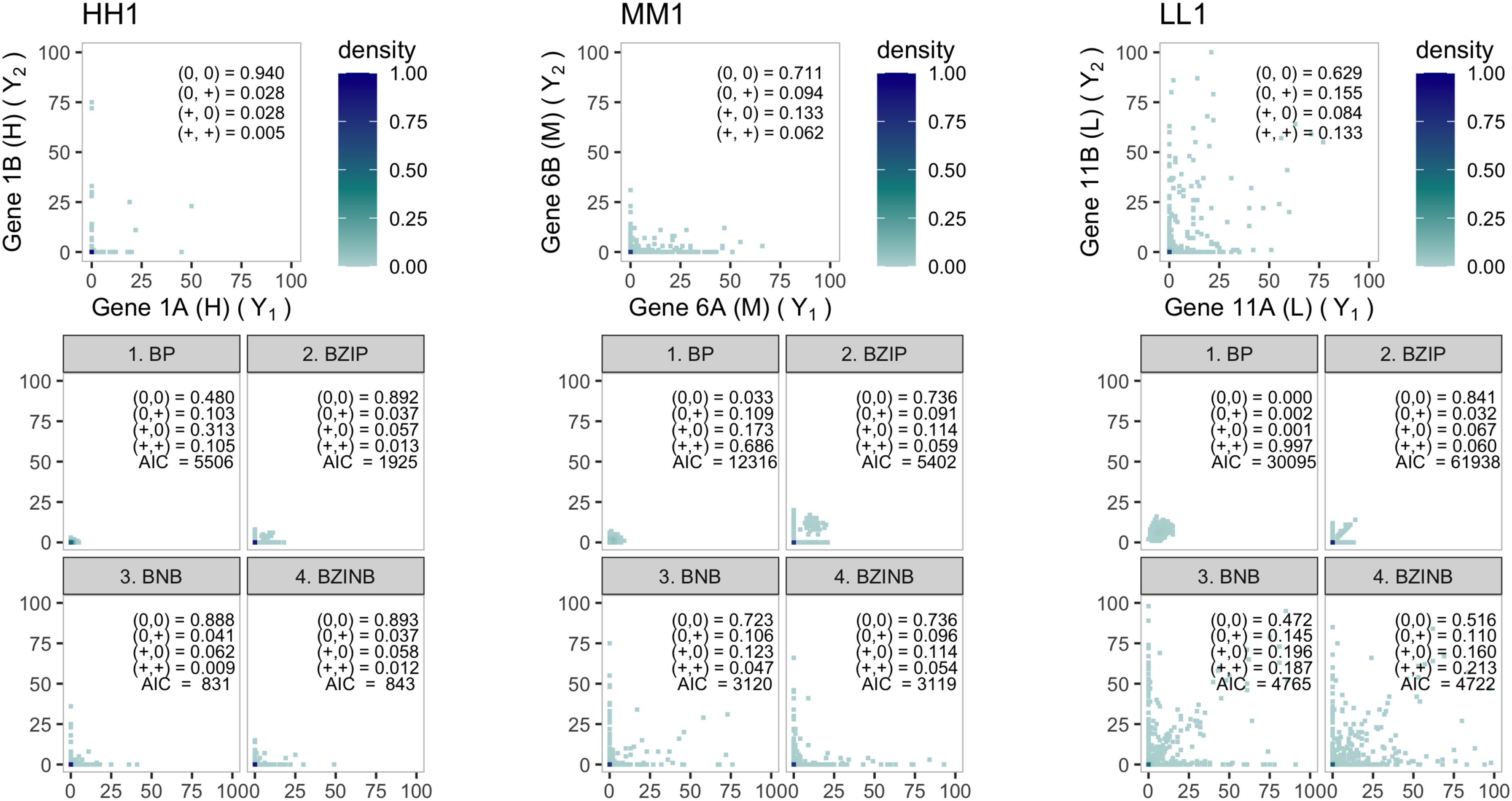
The bivariate distribution of actual and simulated mouse paneth RNA count data. Each of the three panels corresponds to the first gene pair from each stratum: HH1, MM1, and LL1, where the letters represent a stratum with varying proportions of zeros and the numbers represent the number of the pair in each stratum. Each panel has the empirical distribution (top) which serves as truth for the simulations, and the four model-based simulated empirical distributions (bottom). The first four lines of numbers represent the distribution of the dichotomized values (
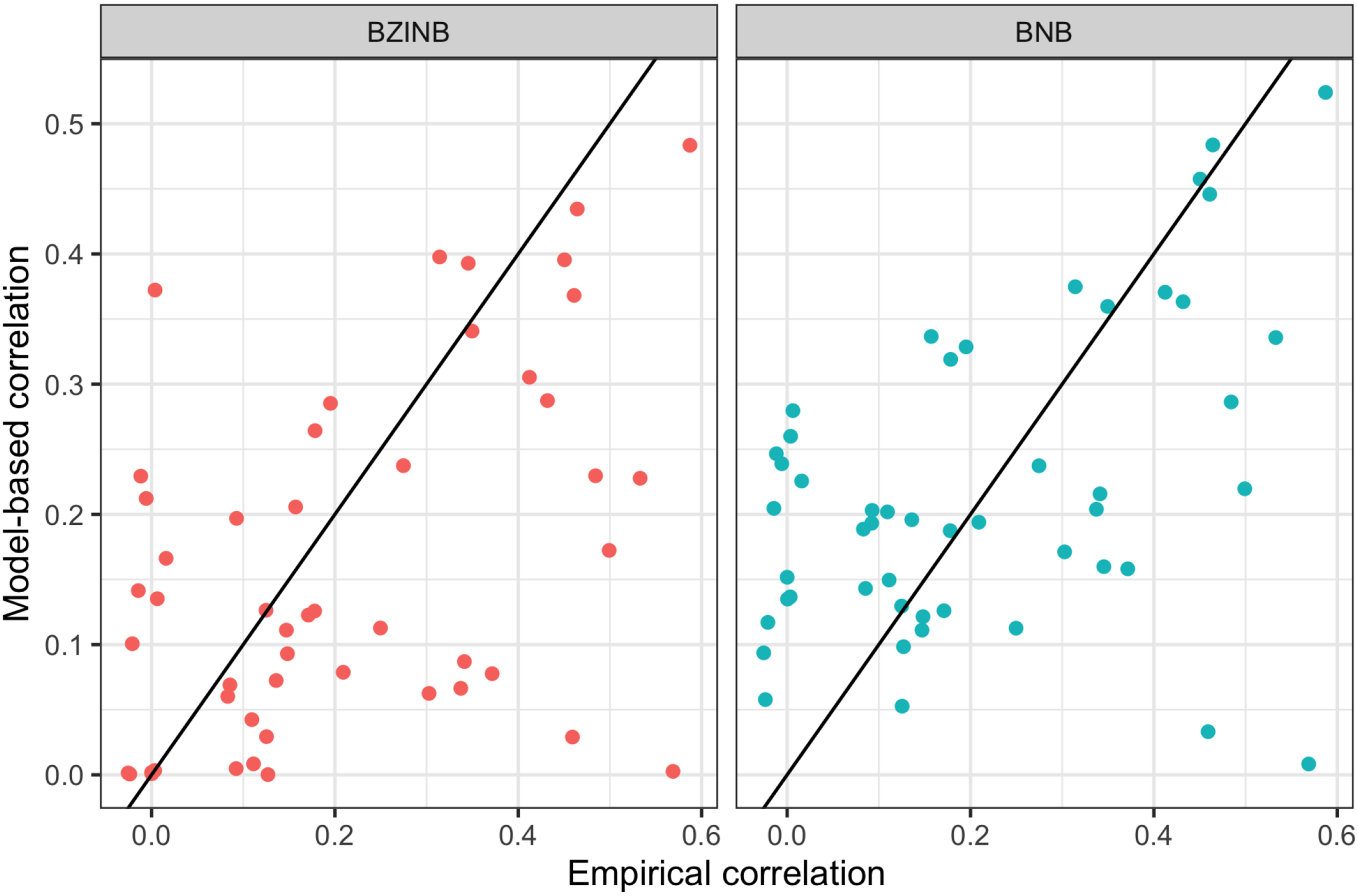
For any pair, the BP model obviously fails to address the overdispersion and zero-inflation, while the BZIP model could not properly mimic the overdispersion. BNB and BZINB seem to fairly mimic the true distribution in most of the pairs. Although BNB provides a decent fit to the data, the seemingly good fit may come at a price of sacrificing the dependence structure. The Akaike Information Criterion (AIC) could be used for model comparisons, and it suggests BZINB for pairs MM1 and LL1 and BNB for pair HH1. Figure 3 compares the marginal correlations of the 50 gene pairs implied by both the BZINB and BNB models; that is, correlations are calculated accounting for both zero-inflation and nonzero-inflated counts. While the BZINB model seems to preserve the magnitude of the observed correlation, BNB has correlations conspicuously lower than the corresponding empirical Pearson correlations. This indicates that the BZINB model carefully considers the overall structure of the data.
Furthermore, when genes have some large-valued counts and many zeros at the same time either marginally or jointly, the BZINB has an apparent advantage over the BNB model. Often, in the BNB model, nonzero count pairs are highly concentrated on the diagonal line, while nonzero counts in the BZINB model are more dispersed away from the diagonal line (LL1 in Figure 2 and more examples in Figures S1 to S2). This can be explained by the lack of flexibility of the BNB model. When data are highly zero-inflated but overdispersed at the same time, BNB is forced to have small shape parameters (
When the excess zeros are believed to come from dropouts, the BZINB model may uncover the underlying dependence using measures such as
For the same 50 pairs in the previous subsection, we estimated the dependence using naive measures—Pearson correlation (PC) and empirical mutual information (EMI)—and zero-inflation adjusted measures—underlying correlation (
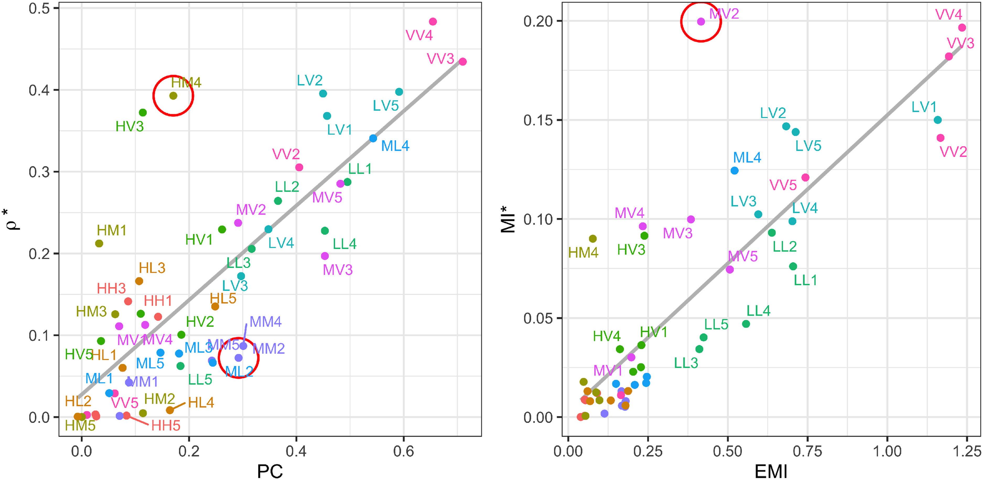
Estimated dependence measures of 50 pairs. Pearson correlation (PC) and underlying correlation estimates (
In Figure 4 left, we see that PC and
Similar analyses can be done for MI-based measures. While EMI and
We ran simulations to study the performance of estimators of underlying correlation and their associated standard error under a finite sample size. We considered 40 distinct sets of BZINB parameter values (Table 1). Note that for each value of
The set of parameters for simulation. Combination of
and
below makes
sets in total.
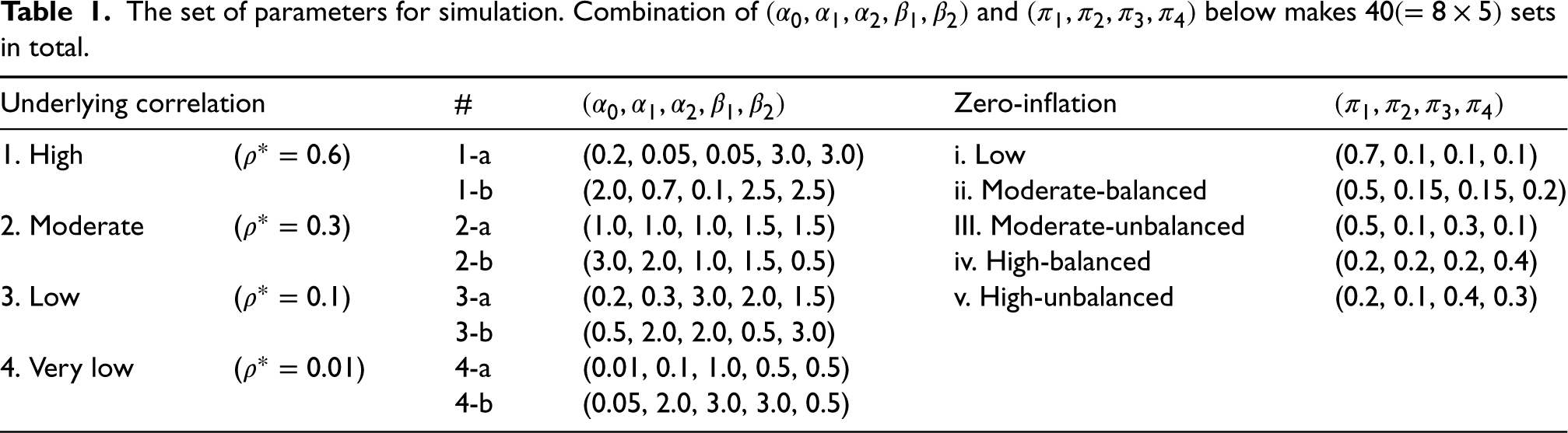
The set of parameters for simulation. Combination of
For each the average estimated standard error (SE, the standard deviation of the parameter estimates (SD, the empirical coverage probability (CP,
In the simulation results, the mean parameter estimates are close, or getting closer as the sample size grows, to their true parameter values for each of the 40 scenarios (Figure 5). For most of the 40 parameter sets, CP was close to 0.95, and for those not close, CP gets closer to 0.95 with increasing sample size. In the same context, the average estimated standard error (SE) was close to the standard deviation of the parameter estimates (SD) especially when the sample size was large (Figure 6). However, when the underlying correlation was close to zero (i.e. 0.01 in our example), standard error estimation did not perform as well in terms of both CP and closeness of SE to SD. The parameter value being near the boundary may be responsible for the poorer performance. Also, Scenarios iv and v have higher SE and SD than the others. One possible explanation to this is that the effective sample size for those high zero-inflation scenarios is smaller than the other scenarios; in other words, for samples with many zeros, the actual number of observations needed to validly estimate the shape and scale parameters (
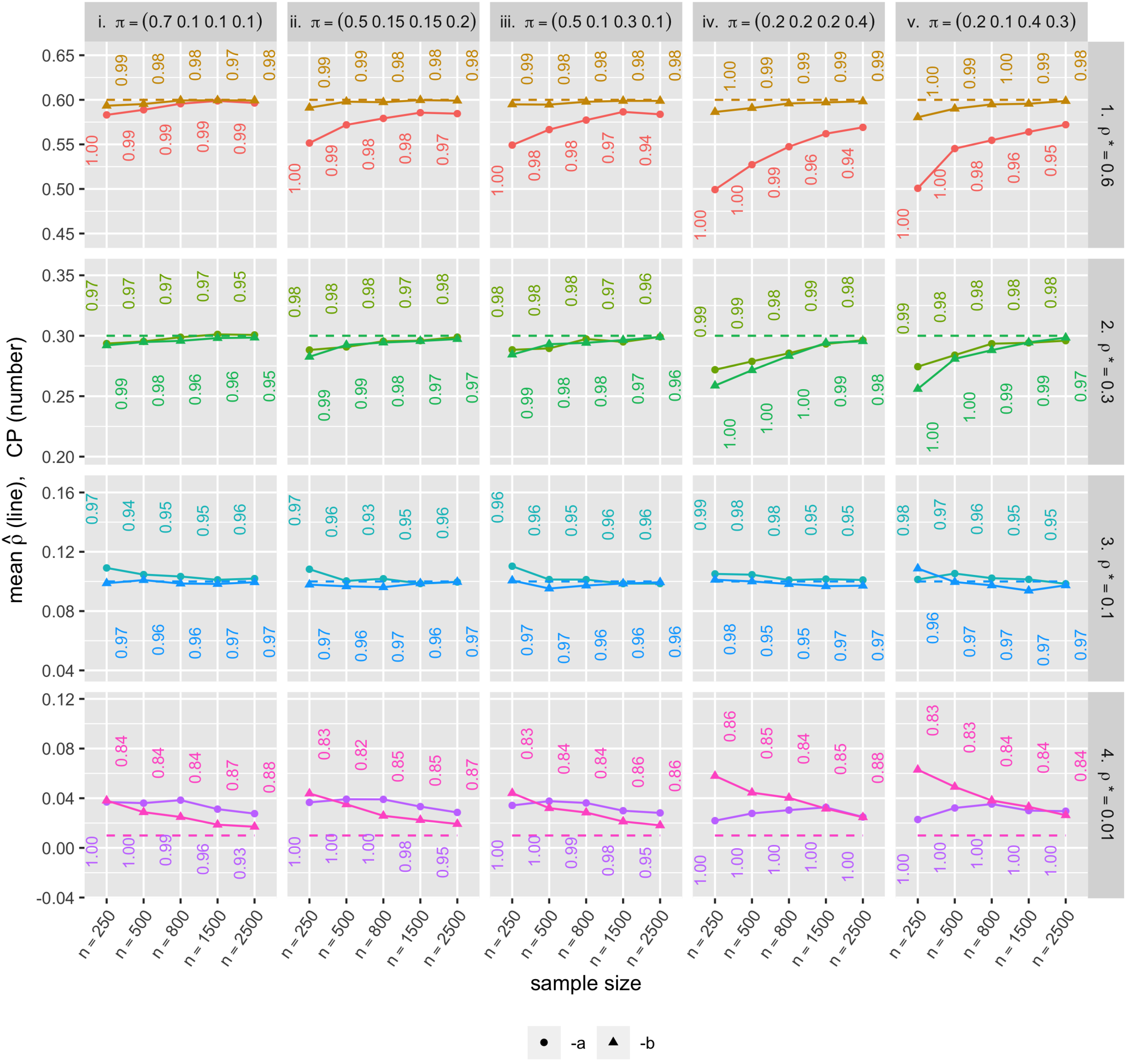
Mean parameter estimates (
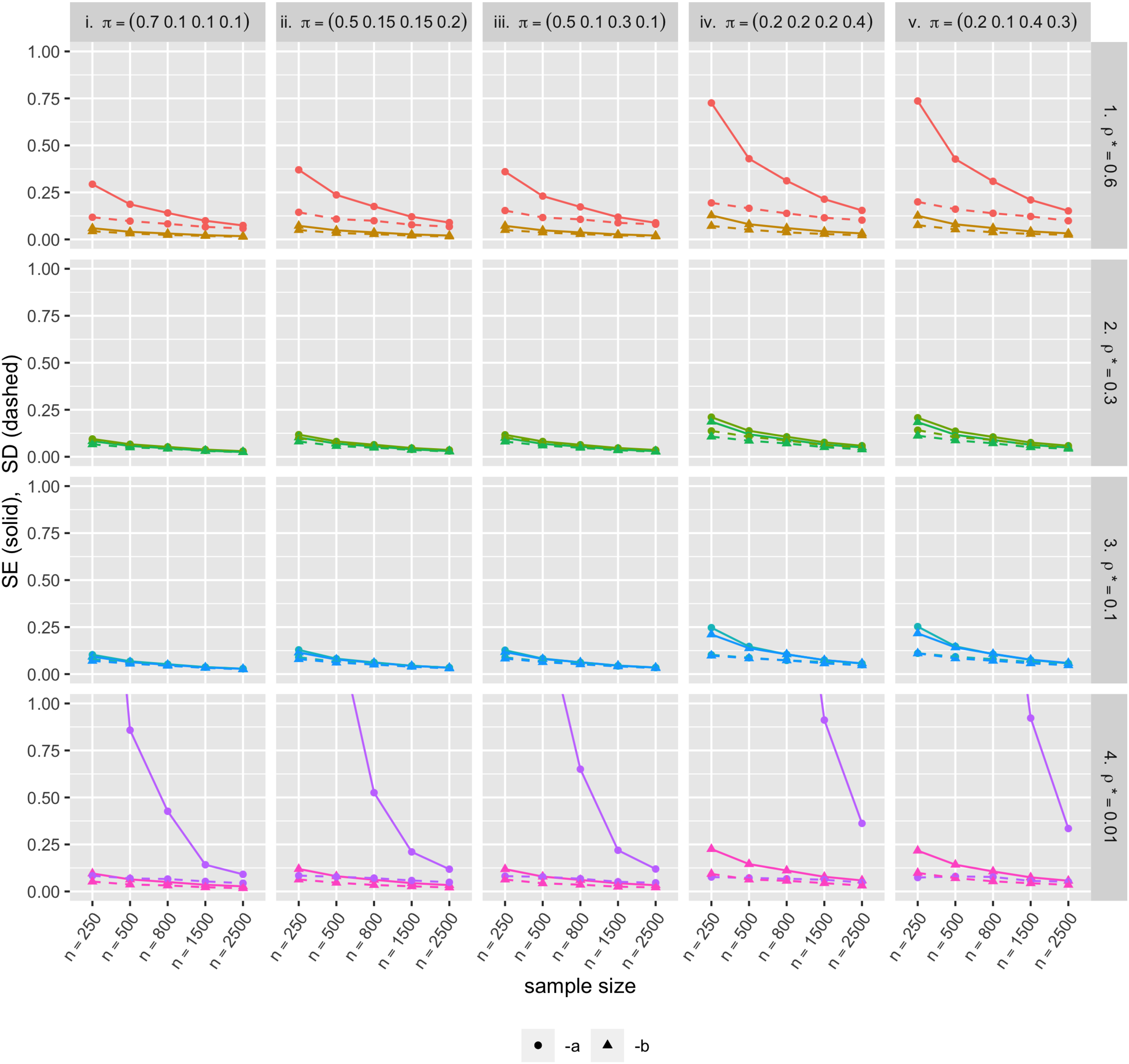
Standard error (SE, solid lines) and standard deviation (SD, dashed lines) of the bivariate zero-inflated negative binomial (BZINB)-based underlying correlation estimates. Each color represents the distinct simulation scenarios.
In the dental caries clinical trial (X-ACT) study,
25
647 participants (ages 21–80 years) were randomized to receive Xylitol versus inactive lozenges with 50% chance. The number of caries 36 months after treatment initiation was recorded for proximal and smooth tooth surfaces with the proportion of no-caries for each type being 23.8% and 22.6%, respectively. Figure 7 compares the empirical distribution with the model-estimates and provides the zero-inflation test results (the mixture chi-square statistics,
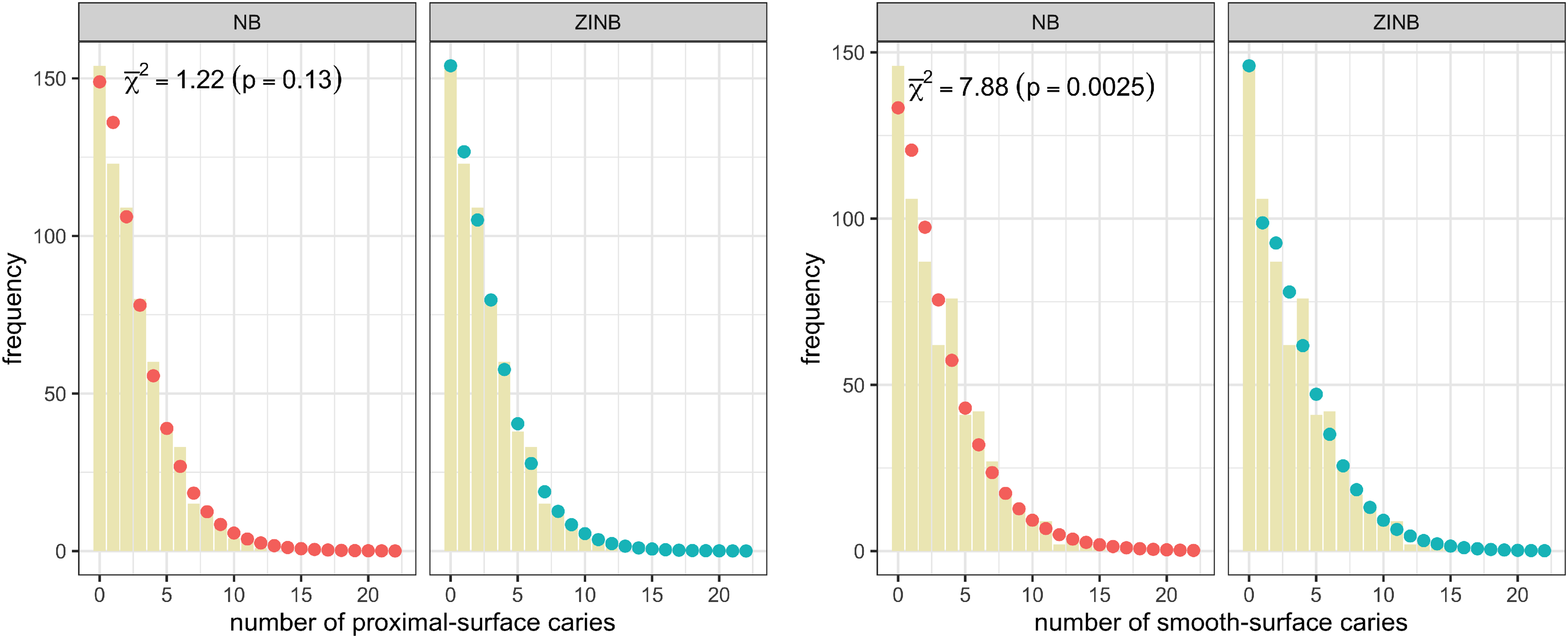
The empirical distribution of the number of caries (bars) on the proximal and smooth surfaces. The fitted NB distribution (red dots, left), the fitted ZINB distribution (blue dots, right), and the zero-inflation test statistics (
The following two approaches shed light on the effectiveness and the efficiency of the bivariate model. First, we rigorously investigate the difference in the joint distribution of the caries counts between the intervention (Xylitol) and control groups, which is not obtainable from univariate models. In the second analysis, we illustrate how bivariate models could be more efficient than univariate models in testing marginal mean differences. The BZINB model parameter estimates for each group are provided in Table 2 and, together with their covariance estimates, the analyses of the joint dichotomized distribution and marginal mean tests are derived.
The BZINB parameter estimates and their standard errors for the Xylitol and control groups.
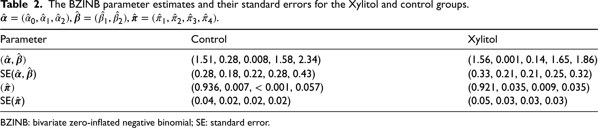
BZINB: bivariate zero-inflated negative binomial; SE: standard error.
Denoting the proximal and smooth surface caries counts as
The bivariate zero-inflated negative binomial (BZINB)-estimated joint probability (and its standard error) of dichotomized caries incidence on smooth- and proximal-surfaces for control (top) and Xylitol (bottom) groups. The estimated probabilities are given by the plug-in estimates of (4) for each group. See Web Section E.3 of the Supplemental Materials for more details.
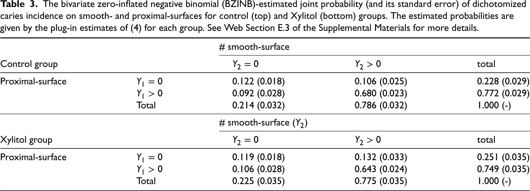
For both proximal and smooth surfaces, an increase in the marginal proportion of caries-free participants is observed in the treatment group. However, interestingly, the proportion of either caries or caries-free for both surfaces jointly has decreased. Provided that there was virtually no change in caries-free-for-both-surfaces, this perhaps implies a shift from caries-for-both-surfaces to caries-for-one-surface. Approximately 3.7%p, where “%p” refers to percentage points, of the caries-for-both group have been transferred to caries-for-smooth-surface-only (2.6%p) or caries-for-proximal-surface-only (1.4%p) groups, with 0.3%p difference is due to decrease in caries-free-for-both group.
In the second analysis, we compare the overall mean caries counts between the Xylitol and control groups for the two outcomes because, in clinical trials, the overall means are typically of interest as opposed to the latent class means. Nonetheless, two-part models for counts provide the structure to test the difference in the marginal means,
It can be seen from Table 4 that while the means are not very different across the models being used, the use of the bivariate model appears to increase the precision of the marginal means estimates. This result is as expected, because in univariate models, the information contained in the other variable not being modeled is not utilized, while bivariate models can leverage the information of the other variable implied by the underlying structure. The standard errors of the BZINB-based estimators (in parentheses) and the p-values of the BZINB-based tests are overall smaller than those of the ZINB-based ones. Most notably, the p-value of the univariate test for smooth surfaces is 0.051 under the BZINB model, compared to 0.106 for the ZINB model.
The univariate and bivariate model-based estimates (and the standard errors in parentheses) of the group means and the group differences. The
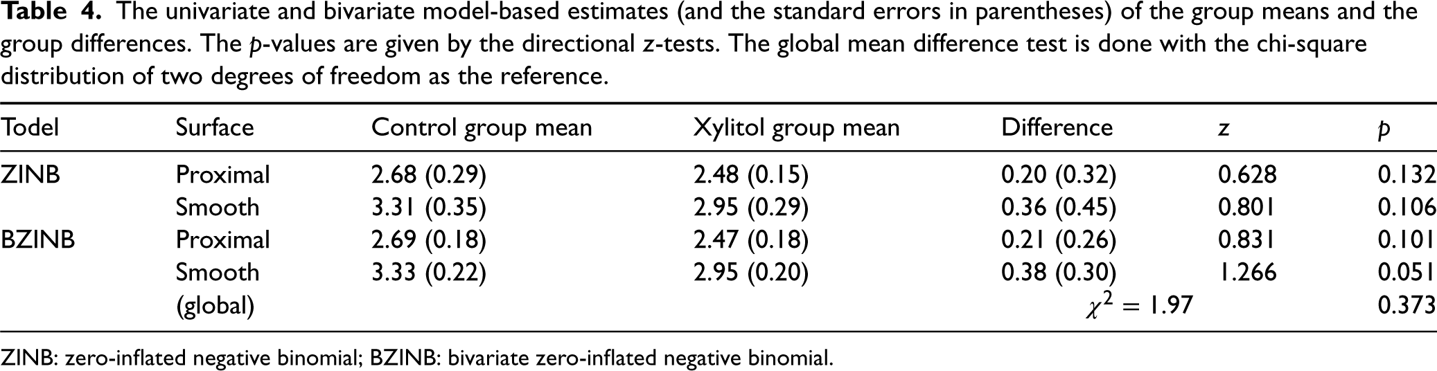
ZINB: zero-inflated negative binomial; BZINB: bivariate zero-inflated negative binomial.
A further advantage of bivariate models is the use of global tests where inference is made by testing against the null hypothesis that the marginal mean parameters of the two groups are the same for all surfaces and rejecting the null if the marginal means differ between groups for at least one of the surface types. In the Xylitol trial, the BZINB-based global test of differences is not statistically significant (
This article proposes a richly parametrized BZINB model that provides a full specification for the distribution of two correlated, overdispersed and zero-inflated, count random variables. Compared to existing ones, it models bivariate count data with high flexibility by having eight free parameters and at the same time with simple latent variable interpretations. The hierarchical nature of the framework allows for the consideration of nested models, such as BNB and BZIP models, and makes the model highly versatile and applicable to various contexts. Moreover, to our knowledge, the BNB model having five parameters is novel.
The BZINB model is applicable to diverse biomedical settings. In the scRNA-seq settings, by decomposing two sources of zeros, the distribution of counts without dropouts is recovered and the dependence is estimated accordingly. In a second example with a totally different perspective on the meaning and utility of modeling “excess zeros” than the first example, the joint pattern of two types of dental caries was examined using the BZINB model in the Xylitol lozenges clinical trial. In particular, the BZINB model applied to bivariate caries counts from the Xylitol study enabled estimation of marginal parameters of common interest in clinical trials including the joint probabilities for the presence versus absence of any caries and overall mean caries counts for each surface type.
The BZINB model proposed in this article assumes an independent and identically distributed random bivariate sample of zero-inflated counts. Future work could generalize this homogeneous mean model to allow for covariance analysis or joint conditional mean analysis by introducing the generalized linear model framework. As in the univariate ZINB regression, the latent count variables (i.e.
There is a growing amount of literature that many scRNAseq data are not zero-inflated, and dropout events are primarily caused by PCR amplification that could be removed by the UMIs technique.43,42,41 While a good amount of comfort is available that there is no zero-inflation in the data for the droplet-based data such as 10X that uses UMI quantification, there is still a need to address dropouts in other platform-based scRNA-seq data as well as single-cell proteomics and metatranscriptomics data. As we have observed the presence of zero-inflation in Section 4, zero-inflated models such as BZINB are needed in the example dataset.
Our model can be applied to other settings where there is a belief in two sources of zeros such as frailty, for example, the first source corresponds to a cohort of people who are not susceptible to disease and will always have a zero count; the other sources are random zeros among susceptible individuals. In this case, the dependence measure proposed in equation (10) applies to the bivariate outcome among the latent class of individuals that are susceptible to disease.
The proper use of the BZINB model depends on researchers’ understanding of how zeros were generated in the data. For example, if the expressed mRNAs are captured and sequenced without dropouts with a certain platform, the observed zeros in the resulting data would represent genes with no expression. In these settings where the excess zeros are not caused by dropout, the overall mean count and the proportion of subjects with positive counts have meaningful interpretations that may be directly modeled by marginalized ZINB
1
and hurdle models,
44
respectively. Directly modeling the observed pairs of counts, that is, (
In the BZINB model, allowing only positive
Finally, the BZINB model can also be generalized to a multivariate zero-inflated negative binomial model. This model may have an exponentially increasing number of latent variables or parameters as the dimension gets large. Though the lack of parsimony may make the multivariate model look less attractive, the idea can be very practically used in simulating multivariate zero-inflated count data and potentially in statistical analysis based on Bayesian models. For instance, a genomic count data with a large amount of zeros can be mimicked by a set of latent random layers along with the generalized linear model framework. In dental caries clinical trials, a trivariate ZINB model could analyze caries counts from three tooth surface types simultaneously with a single global test avoiding the need for multiplicity adjustments to control family-wise Type I error.
Software
An
Supplemental Material
sj-pdf-1-smm-10.1177_09622802231172028 - Supplemental material for A bivariate zero-inflated negative binomial model and its applications to biomedical settings
Supplemental material, sj-pdf-1-smm-10.1177_09622802231172028 for A bivariate zero-inflated negative binomial model and its applications to biomedical settings by Hunyong Cho, Chuwen Liu, John S Preisser and Di Wu in Statistical Methods in Medical Research
Footnotes
Acknowledgments
The authors thank Scott Magness and Joshua Starmer for providing the mouse paneth scRNA seq data, André V. Ritter for sharing the X-ACT study data, and Michael I. Love for discussion of the implications of the dropouts.
Declaration of conflicting interests
The author(s) declared no potential conflicts of interest with respect to the research, authorship, and/or publication of this article.
Funding
The author(s) disclosed receipt of the following financial support for the research, authorship, and/or publication of this article: This work was supported by grant from the National Institutes of Health, National Institute of Dental and Craniofacial Research, R03-DE028983, and University of North Carolina Computational Medicine Program Award 2020.
Supplemental material
The reader is referred to the online Supplemental Materials for A. the standard error calculation, B. details of the EM algorithm, C. additional details of the Xylitol experiment data analyses, and Web Figures. Supplemental material is available online.
References
Supplementary Material
Please find the following supplemental material available below.
For Open Access articles published under a Creative Commons License, all supplemental material carries the same license as the article it is associated with.
For non-Open Access articles published, all supplemental material carries a non-exclusive license, and permission requests for re-use of supplemental material or any part of supplemental material shall be sent directly to the copyright owner as specified in the copyright notice associated with the article.