
Abstract
Recently, treatment interruptions such as a clinical hold in randomized clinical trials have been investigated by using a multistate model approach. The phase III clinical trial START (Stimulating Targeted Antigenic Response To non-small-cell cancer) with primary endpoint overall survival was temporarily placed on hold for enrollment and treatment by the US Food and Drug Administration (FDA). Multistate models provide a flexible framework to account for treatment interruptions induced by a time-dependent external covariate. Extending previous work, we propose a censoring and a filtering approach both aimed at estimating the initial treatment effect on overall survival in the hypothetical situation of no clinical hold. A special focus is on creating a link to causal inference. We show that calculating the matrix of transition probabilities in the multistate model after application of censoring (or filtering) yields the desired causal interpretation. Assumptions in support of the identification of a causal effect by censoring (or filtering) are discussed. Thus, we provide the basis to apply causal censoring (or filtering) in more general settings such as the COVID-19 pandemic. A simulation study demonstrates that both causal censoring and filtering perform favorably compared to a naïve method ignoring the external impact.
Keywords
Introduction
A substantial amount of treatment interruptions during a randomized clinical trial, not expected at the planning stage, might cause that the planned statistical analysis does not address the original study objective anymore. The phase III clinical trial START (Stimulating Targeted Antigenic Response To non-small-cell cancer) had to deal with a large number of treatment interruptions as it continued after a clinical hold (CH) was lifted. 1 A CH order issued by the FDA (US Food and Drug Administration) to the sponsor of a clinical trial entails stop of enrollment and that patients may not receive the investigational drug.
The START study served as a motivating example for Nießl et al. 2 to evaluate the potential implications of the CH on the treatment effect on overall survival (OS) and to suggest analysis methods to account for treatment interruptions induced by the CH. They showed the multistate model framework as a suitable and flexible tool to investigate the impact of the CH on the treatment effect supporting discussions around appropriate analysis methods. To compensate for a potential negative impact of the CH on the treatment effect Nießl et al. 2 suggested a censoring approach which censors patients at the start of the CH. They showed that this approach provides reliable estimates of the treatment effect on OS preserving the initial objective of the trial for a causal interpretation: estimation of initial treatment effect in the absence of the CH. Their argumentation is based on the fact that the CH order is an external event. It is important to note that censoring by CH is independent in a counting process sense. This is more subtle than the common random censoring model that assumes stochastically independent death and censoring times. Assuming a beneficial treatment effect, censored and uncensored patients cannot be assumed to have the same hazard of death because censored patients may have to suspend their treatment which is expected to be harmful for the time to death.
The considerations of Nießl et al. 2 serve as motivation to provide an in-depth discussion on the connection of censoring by treatment interruption and causal inference for assessing treatment effects under hypothetical interventions.
In this article, we suggest an enhanced CH-censoring approach, which censors only patients that actually had to interrupt their treatment due to the CH. These are the progression-free patients in the treatment group, because in the START trial, treatment is administered only before disease progression. However, this method implies that we cannot simply use a Cox model to determine the treatment effect.
Moreover, we transfer our considerations about causal censoring to the more general concept of filtering making use of information collected after the end of the CH. These two novel methods to account for the CH have the major benefit that more observed events are included in the analysis compared to the censoring approach of Nießl et al. 2 However, it is less intuitive whether these two new methods provide causal estimates, as the censoring (and filtering) now depends on individual covariate values. To gain a better understanding of the relationship between independent censoring in a counting process sense and censoring as a causal intervention, we examine, based on the example of the CH situation, the implications of the censoring and filtering approaches on the matrix of transition probabilities from both a causal perspective and a multistate model perspective. In doing so, we also address the connection of “censoring by treatment interruption due to CH” to the g-computation formula.3–6 Moreover, we discuss the assumptions for “causal censoring,” that is, for censoring that lead to an identifiable causal effect. Our goal with this paper is to provide a conceptual multistate framework that enables us to address treatment interruptions or discontinuations and to identify a causal treatment effect in general settings with an external time-dependent covariate inducing a time-varying treatment.
Another example for a possible application are clinical trials affected by the COVID-19 pandemic. The current COVID-19 pandemic and subsequent restrictions have various consequences on planned and ongoing clinical trials. Its direct and indirect effects might lead to intercurrent events and missing data potentially leading to biased study results. The multistate model approach could support discussions and decision making on how to cope with the COVID-19 pandemic from a statistical point of view. 7 van Geloven et al. 8 discuss censoring of treatment as a hypothetical strategy for answering the question of how likely an event would be if no one received treatment.
In contrast to Nießl et al., 2 this article will focus on the estimation of probabilities using the Aalen-Johansen estimator rather than the estimation of hazard ratios to be more in the spirit of causality. 9
The remainder of this article is structured as follows. Section 2 introduces the theoretical background including survival multistate models as well as some key aspects of causal inference. Section 3 recapitulates multistate modeling of a CH by the example of the START trial and suggests two novel methods to account for the impact of the CH. Section 4 set out the link to causal inference and the identification of causal treatment effects. In Section 5., simulation studies are performed comparing the suggested methods. The article concludes with a discussion in Section 6.
Theoretical background
We begin by presenting general survival multistate models with a focus on external categorical time-dependent covariates and the estimation of transition probabilities (Section 2.1.). Section 2.2 gives a short overview of some aspects of causal inference we need to create the link between multistate modeling and the identification of causal effects.
Survival multistate models and time-dependent covariates
In contrast to the standard survival model, a multistate model facilitates the analysis of complex survival data with any finite number of states and any transition between these states. 10 If no transitions out of a state are modeled, the state is called absorbing, and transient otherwise.
A multistate model could be interpreted as a joint model for time-dependent categorical covariates and the time-to-event endpoint: covariates are included through transitions from one transient state to another and the time-to-event endpoint through the time until the multistate process enters an absorbing state. Figure 1 shows an illness-death model with absorbing state death and transient state progression of disease (PD) that jointly models the oncology endpoints OS and progression-free survival (PFS). 11 The model also reflects the situation of the START study if the CH had not occurred.
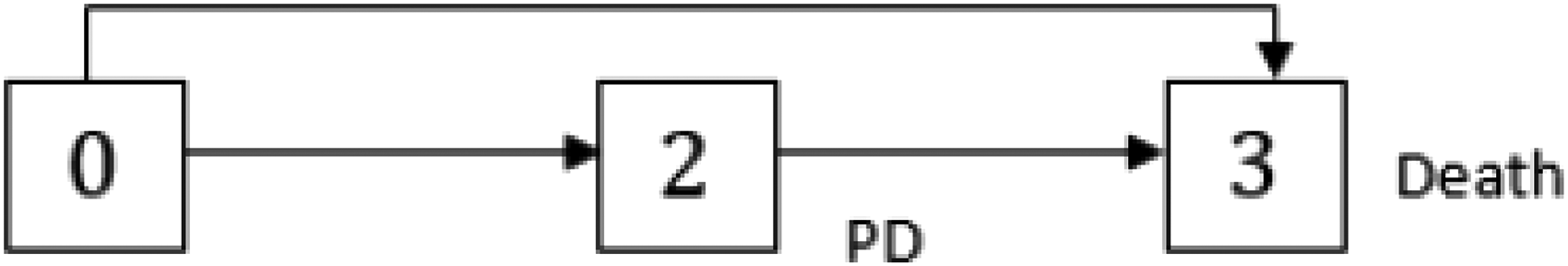
Multistate model with progression of disease (PD) as intermediate state.
Basically, Kalbfleisch and Prentice
12
distinguish between two categories of time-dependent covariates. To put it briefly, in contrast to internal covariates, the existence of external covariates does not depend on the individual under study. A simple example of an external covariate is air pollution in a study of asthma events. The level of air pollution may influence the hazard on asthma events, but asthma events of individuals have no impact on the level of air pollution. An example of an internal covariate is blood measurements at study visits. The PD state in Figure 1 represents the internal time-dependent covariate progression status. Kalbfleisch and Prentice
12
give also a formal definition of external covariates, which is introduced below. Let


As stated above, time-dependent and typically internal covariates with finite range could be incorporated in a multistate model. Including an external time-dependent covariate into a multistate model converts it to an internal covariate to a certain extent, as the covariable then reflects the individual experience of the patient under study. 13 The event of the CH can be described by an external time-dependent covariate, but, as we will discuss later, by adding the CH to the multistate model, we no longer consider it as an external event but its internal effect of treatment interruption.
Let


Furthermore, we introduce the following counting process notation. We consider n replicates assumed to be independent with individual process


Causal analysis goes one step further as the standard statistical analysis and does distinguish between causal effects and other sources of association. Many relevant publications dealing with causality from a statistical point of view use different causal notations and frameworks.17–19
Within this section, we focus mainly on the general requirements to identify a desired causal effect from observational data without going into details.
Pearl
18
has introduced a notation that describes the situation where a single variable
A common graphical tool for displaying causal relations are causal DAGs (directed acyclic graphs). A detailed introduction to DAGs can be found for example in Greenland et al.
20
or Maathuis et al.
21
There are graphical rules like the back-door criterion which help us to decide whether we could identify a causal effect under the assumed causal model. Random variables are displayed as nodes and directed edges (arrows) convey the causal directionality. The lack of an arrow from one node to another can be interpreted as the absence of a direct causal effect regarding those nodes. Figure 2 shows an example DAG that reflects the situation of the START trial at a fixed time t. We will discuss this DAG in detail in Section 4.1. Let

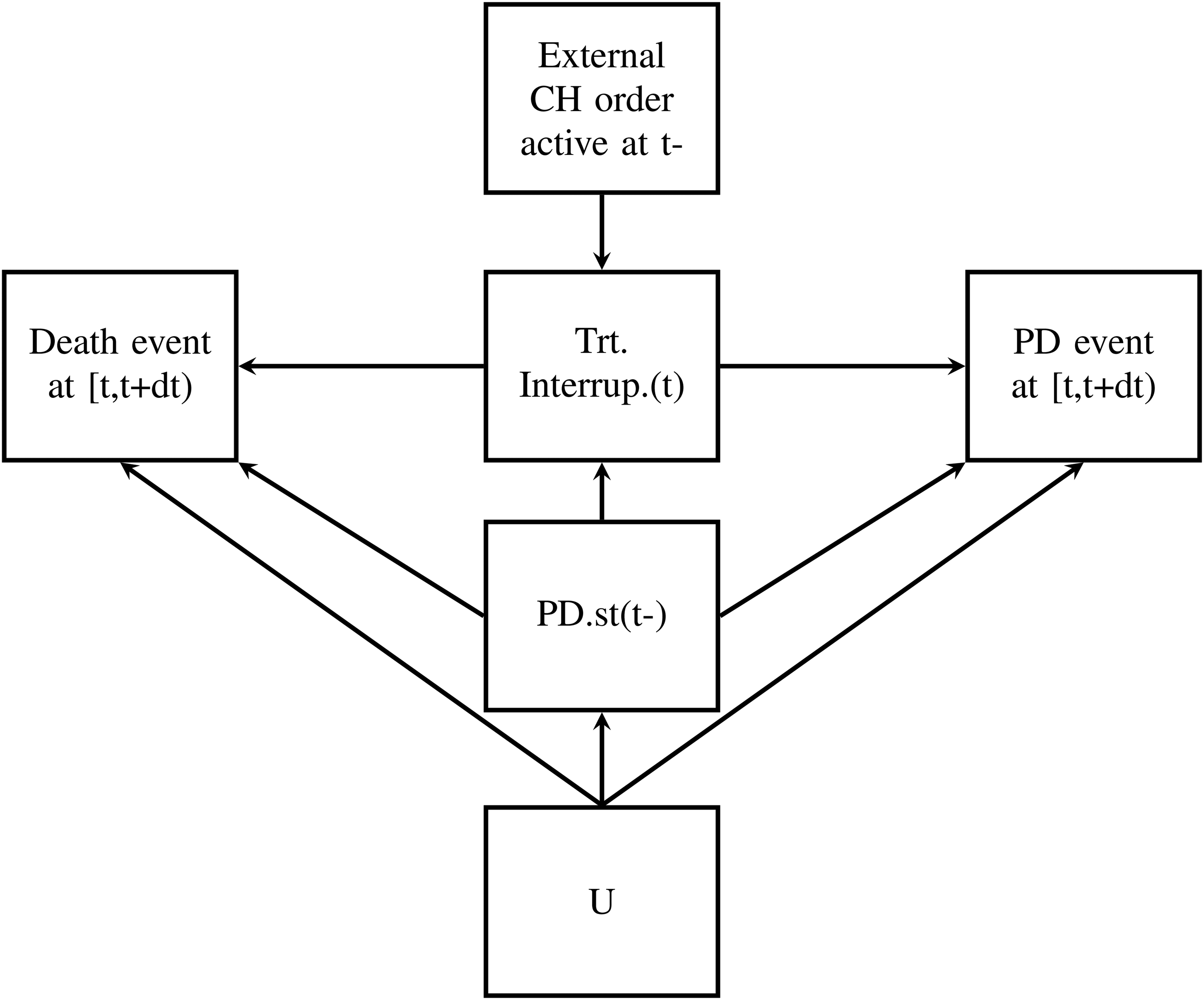
DAG for CH situation at fixed t. Note: The DAG describes causal relations for patients still alive at time t. DAG: directed acyclic graph; CH: clinical hold.
A variable that has no parent is called exogenous or root node and is determined only by factors outside of the graph. Otherwise, a variable is endogenous.
To quantify causal relations by analyzing observational data, we need some stronger assumptions than for standard statistical analyses. Hernán and Robins
17
describe three identifying assumptions for estimating averaged causal effects.
Positivity: the combination of values possible under the intervention must also be possible under the observational regime. That means the relevant combinations under the observational regime requires a positive possibility. In our example, we observe non-progressive and progressive patients with death event that are not affected by the CH. Exchangeability: The individuals with intervention would have experienced the same average outcome as the individuals without intervention if they had not been subject to intervention. Randomization in clinical trials is expected to produce exchangeability between the treated and the untreated. Conditional exchangeability means that exchangeability is guaranteed within the levels of a covariate. Consequently, this assumption implies that there are no unmeasured confounders that are a common cause of both the exposure subject to the intervention and the outcome. In our example, the question is which patients can be assumed to experience the same average treatment effect as patients affected by CH would have if there were no CH. Consistency: the intervention must be well-defined involving that actual and counterfactual survival times coincides when the actual observed exposure is equal to the intervention value. We will define a concrete intervention representing “no CH” in later sections and we will see that there is more than one option.
A causal DAG
Furthermore, the graphical model

For any intervention on

According to the definition of a causal DAG by Didelez, 24 the DAG is causal, implying that all causal effects are identifiable, if (9) and (10) hold.
Section 3.1 describes the motivating data example, the START trial sponsored by Merck KGaA. Section 3.2 recapitulates how the CH is incorporated in a multistate model as proposed in Nießl et al. 2 Section 3.3 suggests two methods to account for CH impact extending the censoring approach proposed by Nießl et al. 2
Motivating data example: The START trial
The START trial was a phase III, 2:1 randomized, placebo-controlled, and double-blind group-sequential trial. The aim of START was to investigate whether the MUC1 antigen-specific cancer immunotherapy tecemotide given as maintenance therapy after chemoradiation improves OS duration in patients with unresectable stage III non-small-cell lung cancer. 1 Treatment was administrated until PD.
At the time of the CH, accrual was nearly completed with 1182 of 1322 planned subjects, blinded treatment was suspended in 531 patients and 180 patients did not restart treatment after a median of 135 days of treatment interruption when the CH was lifted.
The sponsor decided to continue the trial after increasing the overall sample size and to exclude those patients in a modified intention-to-treat (mITT) analysis believed to be most affected by the treatment interruption, that is, all 274 patients randomly assigned within the six months before the CH were excluded from primary analysis. Overall, 1513 patients were enrolled, with 1006 treated with tecemotide and 507 assigned to placebo. In the mITT subset 1239 patients remained, 829 receiving tecemotide and 410 receiving placebo. Results of the trial showed no significant prolongation of OS duration in the mITT analysis population used for primary analyses. Thus, the question arises if the mITT analysis had in principle compensated for potential implications of the CH.
Nießl et al. 2 showed that the mITT analysis was a reasonable proceeding providing reliable estimates of the initial treatment effect for OS. Moreover, they suggested a more flexible censoring approach for compensating the impact of the CH. More details about the START trial are available in Butts et al. 1
Multistate models for treatment and control groups
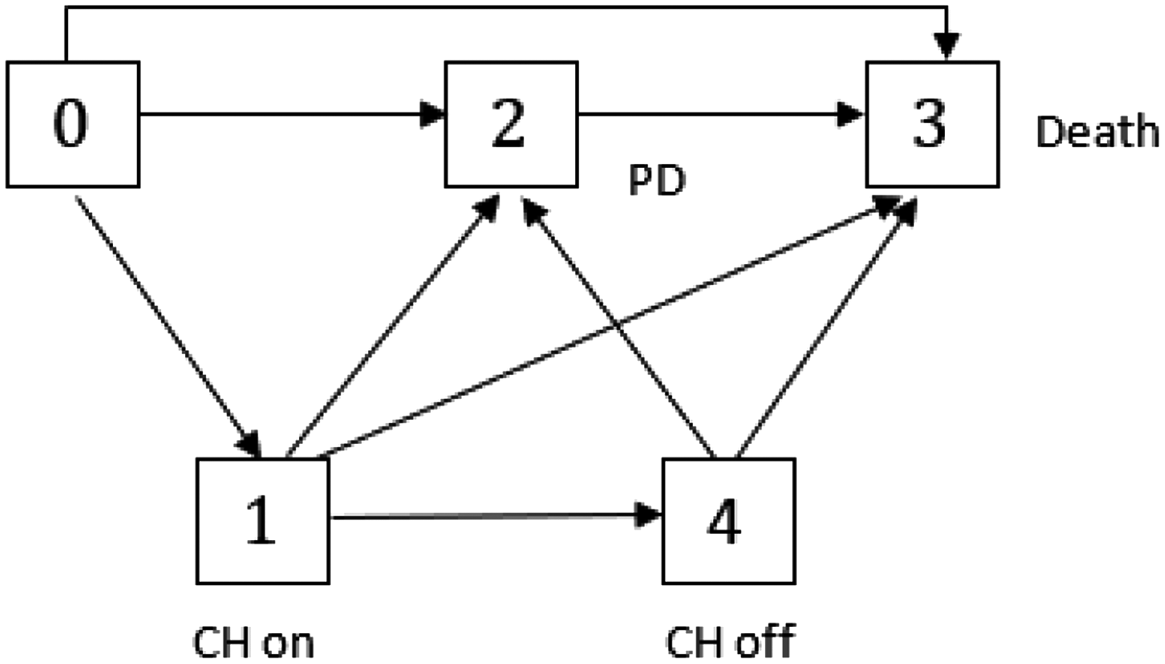
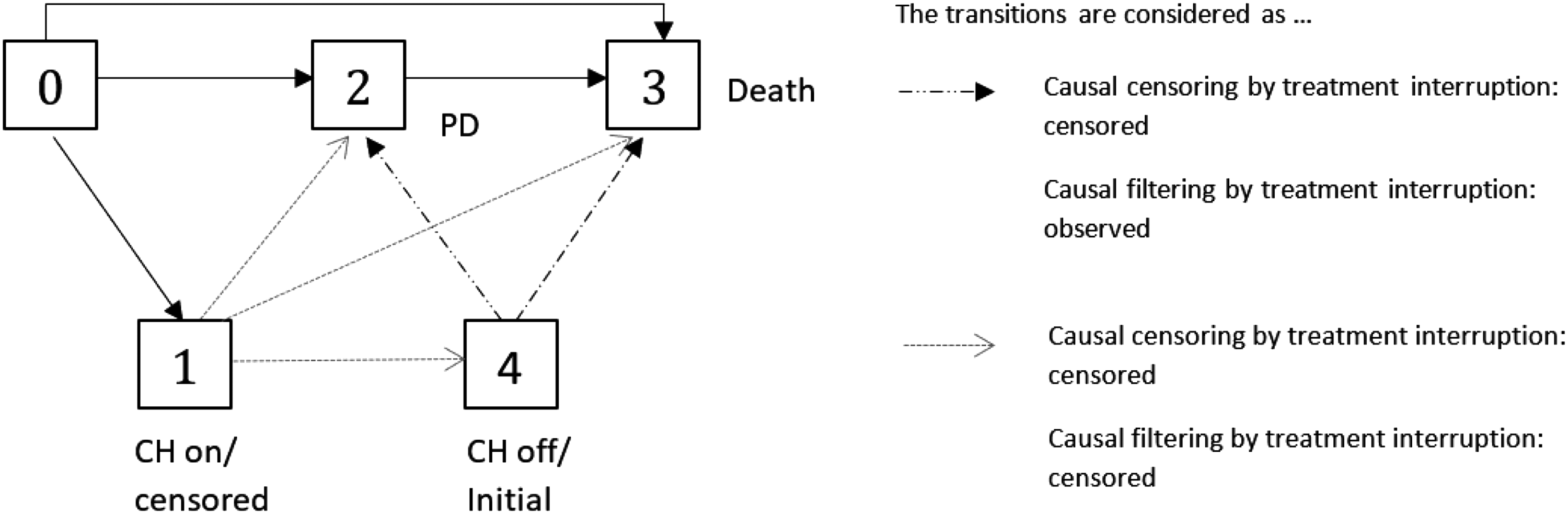
To evaluate the impact of the CH on the treatment effect, we consider two separate models for treatment and control groups as proposed in Nießl et al. 2 Both models include PD as a transient state, as treatment changed upon PD for the treatment group as well as for the placebo group. It has to be noted that both treatment decisions and PD state in our multistate model refer to the time of the diagnosis of PD. To describe the event of the CH in the treatment group we add two transient states representing the start and end of the CH to our model (see Figure 4). Assuming that an induced treatment interruption of active treatment is the major consequence of the CH, we do not model the CH in the control group (see Figure 3). In the START trial, blinded treatment was discontinued with PD. As a consequence, patients with PD or death prior to CH did not experience a treatment interruption due to the CH. We model the CH as an individual event of a patient’s course of disease and treatment, as only patients actually affected by the CH make a transition into the state “CH on.” Thus, we have to distinguish between two types of covariates describing the CH, on the one hand, the CH as an external covariate that occurs at one point in calendar time for the entire population, and on the other hand, the CH as an internal covariate incorporated in our multistate model that induces a treatment interruption. 13
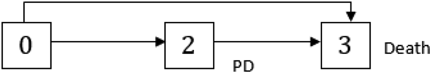
Multistate model with progression of disease (PD) as intermediate state for the control group.
Multistate model
In Nießl et al. 2 the multistate model has been used to generate a better understanding of the impact of the CH on the treatment effect in the START ITT population. We briefly recap the main results: The Nelson-Aalen estimates of the direct death hazards (i.e. death without prior progression) are rather low and no clear difference can be observed between treatment groups. Also, no clear treatment effect could be observed for the time from the PD state to death (2 → 3). However, the Nelson-Aalen estimates of the cumulative hazards into the PD state indicate a protective effect of treatment on the time until PD, which cannot be observed during treatment suspension due to CH, but is restored with the resumption of treatment. In other words, when comparing the Nelson-Aalen estimates of the “0 → 2” and “4 → 2” cumulative transition hazards to the “0 → 2” cumulative transition hazard of the control group, a treatment effect is observed that does not occur when comparing the estimates of the “1 → 2” cumulative transition hazard to the “0 → 2” cumulative transition hazard of the control group. We refer to Nießl et al. 2 for a detailed discussion of the Nelson-Aalen estimates and a graphical illustration incorporating incidence rates into Figures 3 and 4 for easier interpretation.
Our aim is to identify the initial treatment effect on OS in a hypothetical situation where the CH has not occurred. With regard to our multistate models OS is defined as the time until the absorbing state “death” is reached.
Nießl et al. 2 compared the mITT analysis as applied to the START data and the censoring approach to the naïve approach which simply ignores the CH. They concluded that the mITT analysis was a meaningful approach that compensated for the impact of the CH. However, the censoring approach is a simple alternative that provides convincing simulation results and needs less information about the mode of action of the treatment than the mITT analysis where an exclusion window has to be determined. Moreover, Nießl et al. 2 pointed out that the censoring approach has a causal interpretation with regard to a treatment effect that had been observed in the absence of the CH. Thus, we want to extend the censoring concept and will also have a closer look at the connection to causal inference to enable the application of causal censoring in more general settings.
In Nießl et al.
2
all patients—actually affected by the CH or not—are censored at the beginning of the CH exploiting the fact that CH is an external mechanism independent of the individual patient. Let
Multistate model
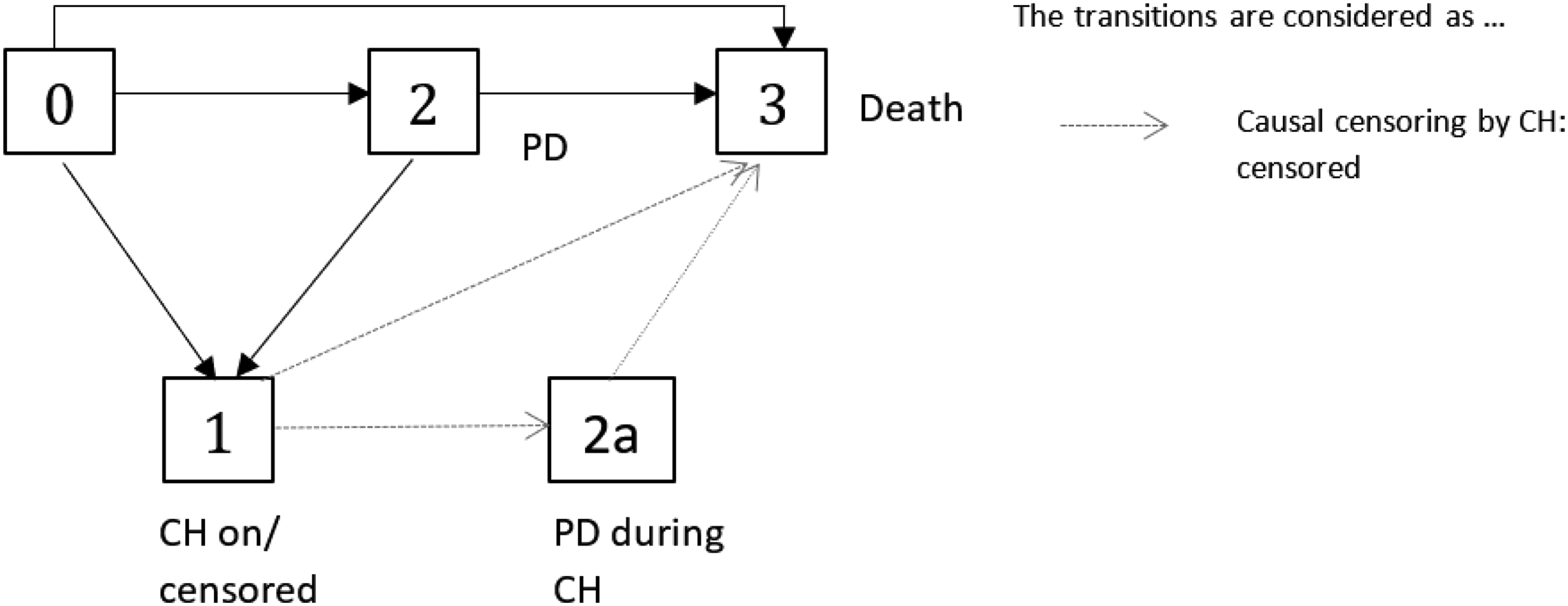
A possibility to reduce the censoring rate is to censor only patients which are actually affected by the CH, that is, who had to suspend the experimental treatment. With regard to our multistate model (cf. Figures 4 or 6), an individual is censored as soon as it enters the state “CH on.” An illustration of the concept of “censoring by treatment interruption” is given in Figure 6. With this censoring, state 1 (“CH on”) is an absorbing state and only the solid black arrows are considered as “observed.” Let
Multistate model (


We will show in Section 4.2 that we can use the partial empirical transition matrix, that is the Aalen-Johansen estimator applied to the censored data (here: censoring by treatment interruption (12)), for causal inference in the hypothetical situation.
The “censoring by treatment interruption” does not use any information collected after the resumption of treatment. We propose a further approach which might be preferable in settings where restoring of the treatment effect can be assumed, e.g. in chronic, non-life threatening disease. It should be noted that the multistate framework is a suitable tool to evaluate whether a treatment effect is restored after a treatment interruption. Our suggestion is to censor the patients as described before, but to re-include them to the analysis/risk sets after the end of treatment interruption due to CH with the end of CH as entry time, if they are still under observation at the end of their treatment interruption. As illustrated in Figure 6, according to this approach transitions out of state 1 are not considered in the analysis but, in contrast to the “censoring by treatment interruption” approach, transitions out of state 4, that is now treated as the initial state after “observation has been switched on,” and “2 → 3” transitions after CH are considered. It is important to note that it is not possible for a patient to contribute to the risk set twice at the same time, as re-entry does not mean that a patient’s study time is reset. This approach corresponds to filtering, as it does not consider any death or PD events during CH. Let us define
In the following we summarize the censoring and filtering concepts introduced in this section. The concepts have in common that they provide the basis for valid causal estimates of the treatment effect that would had been observed in the absence of the CH, but the way the intervention “no CH” is implemented differs. In other words, under certain assumptions they all could provide inference for Censoring by CH: A patient is censored if Censoring by treatment interruption: A patient is censored if Filtering by treatment interruption: We observe the patient’s course of disease via the filter
As illustrated in Figures 5 and 6, the crucial difference between “censoring by CH” and “censoring by treatment interruption” is that in Figure 5 a progressive patient could make a transition into the CH state (i.e. will be censored), in contrast to Figure 6.
It has to be kept in mind that the CH per se is an external event that could be described via an external time-dependent covariate (see Section 2.1.). However, our defined covariates
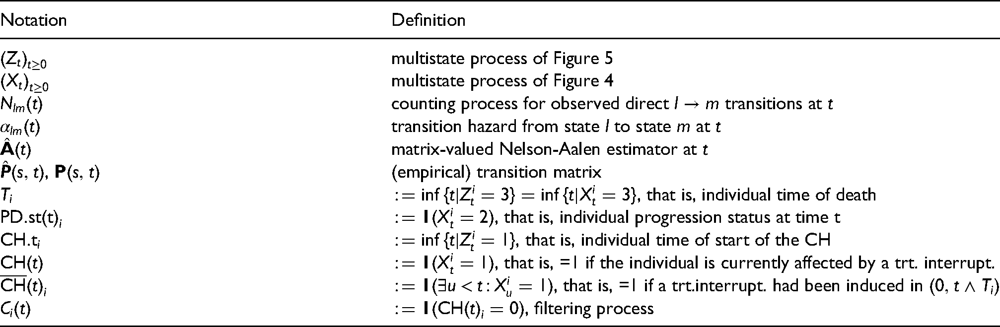
Table 1 summarizes part of the introduced notation, which we will need later on.
Notation table (only with main notation).
Before showing that the estimation of the transition matrix when censoring by CH coincides with the estimation of a causal treatment effect under the hypothetical intervention “no CH occurred” (cf. Section 4.2.) , we present a DAG to illustrate the underlying data generating mechanism (cf. Section 4.1.).
Causal DAG
We use a causal DAG (see Figure 2) to represent the CH study situation and to discuss it from a causal point of view. In contrast to a multistate model, where the arrows illustrate the potential subsequent occurrences of events, an arrow in the DAG indicates causal influences (cf. Section 2.2.).
We consider the causal relationships at a fixed time-point t. Consequently, the DAG does not represent the complete study situation. However, it will help us to understand the source of potential bias and to define an adequate Markov multistate model that captures all information to prevent bias introduced by censoring.
As already stated, the occurrence of the external event CH (not its implications) does not depend on any individual covariate paths. From a causal perspective, the “external” CH is an exogenous variable, that is, a root node with no descendants, as it does not have any causal parents within our model (i.e. within our clinical trial). The CH induces a treatment interruption if a patient is still under risk and progressive-free at the time of the CH. Thus, progression status just before the beginning of the CH is a causal parent of “treatment interruption induced by CH.” In other words, the progression status has to be known to understand whether the individual is affected by the CH or not. A treatment interruption might influence the treatment effect on time till death and on time till progression. The DAG must be interpreted locally in time and therefore does not indicate whether a past treatment interruption still influences time to death or PD event after resumption of treatment. The current progression status may affect the time to death as well. Moreover, it can be assumed that progression status just before t and PD or death event at t have common causal parents (denoted by U in Figure 2).
Figure 2 shows the DAG which summarizes the causal relations in our clinical trial within the treatment group at fixed time t. It is important to note that the CH per se is an exogenous variable, but because its impact depends on individual covariates, the induced treatment interruption is endogenous.
Causal interpretation of the partial empirical transition matrix
In the following section, we discuss the causal interpretation of the partial empirical transition matrix that results from applying our censoring and filtering approaches. We begin by considering g-computation in the setting of time-continuous Markov chains and its connection to our censoring and filtering approaches. Aalen et al. 5 pointed out in their rather brief Section 9.6.2 that estimating a partial transition matrix, that is, the usual estimator of transition probabilities but applied to artificially censored data, for example, because of treatment deviations, gives a valid estimate for the treatment effect in the absence of treatment deviations, that is, under do(no treatment deviation), and that this estimator could be seen as a special case of the g-computation formula. 6 Moreover, Gran et al. 4 present the artificially manipulating transitions in a multistate model for sickness absence at work as a possible method to assess the causal effect of certain interventions. However, the arguments for the causal interpretation of the partial transition matrix after censoring have so far been indicated in the mentioned literature rather than explored and justified in detail. It is important to note that generally censoring in a multistate model framework provides a causal interpretation of the partial empirical transition matrix, but requires certain causal assumptions. Therefore, we will have a closer look at the connection of censoring multistate model data and g-computation and will investigate the assumptions for the identification of a causal treatment effect in the presence of treatment interruptions.
Our objective is to estimate the initial treatment effect on OS which would have been observed in the absence of the CH. Thus, we could consider the state occupation probability of the absorbing state death under do (no CH):
For ease of presentation, we will not consider event times subject to right-censoring. That means we do not consider “usual” right-censoring additional to the censoring by CH. It is important to note that all derivations within the following sections could easily be extended for independent right-censoring using the well-known standard arguments.
G-computation and censoring by treatment interruption
For the moment, we will ignore the external node U of the causal DAG (cf. Figure 2) which is a common causal parent of both PD and death events, and show that then our censoring approach coincides with the g-computation formula.
Estimating the transition matrix while treating patients affected by the CH as censored results in a partial transition matrix in the sense that less transitions are considered and the state space is reduced compared to the usual transition matrix for our multistate model of Figure 4. We want to show that considering this partial empirical transition matrix corresponds to the g-computation and provides valid estimates with a causal interpretation towards a hypothetical treatment effect without CH. We use the same notation as introduced in Section 3.3. (cf. Table 1).
We drop index i and recall that 

Hence
One way to implement our desired intervention of “no treatment interruption induced by CH” is setting
According to the g-computation formula (10), we get We do not consider We set
Steps 1 and 2 imply that we can leave out those matrices describing transition times 

As we have seen in Section 3.3., “censoring by treatment interruption” is independent in the sense that the estimation of the
More details including a very simple and constructed data example can be found in the Supplemental Materials.
Similar considerations to those described in the previous section for causal censoring also apply to our causal filtering approach. As explained in Section 3.3., the difference to the causal censoring approach is that additional to the censoring at the start of the treatment interruption due to CH, patients still under observation at the end of the CH will be analyzed just as they would re-entry the study, that is, transitions out of the state “CH off” are treated as transitions out of the initial state (see Figure 6). Under the assumption that the treatment effect is restored as soon as the treatment is restarted an alternative intervention corresponding to do(no CH) is setting
The (partial) empirical transition matrix of the filtered process
Using the same reasoning as in Section 4.2.1., but denoting by
More details including a very simple and constructed data example can be found in the Supplemental Materials.
The partial empirical transition matrix and the back-door criterion
We showed that, when ignoring the exogenous causal node U, the partial transition matrix is a direct application of the g-computation formula or truncated factorization formula (10). However, we know that in our setting there are nodes in the causal DAG (Figure 2) with common unobserved exogenous causal parents denoted by U. That means, there are potential unobserved confounders. The argumentation in the previous sections is primarily based on the fact that after application of the g-computation formula all factors
Looking at the causal DAG (Figure 2) we find that the current progression status (PD.st


However, in Section 4.2.1 we do not just omit some factors from
This underlines again that the causal graph at a fixed time t is an aid to find the appropriate multistate model leading to a causal analysis, but describes not completely the causal relations of the complex situation.
In summary, we pointed out by using the back-door criterion that the unmeasured parents U can safely be ignored when calculating the partial empirical transition matrix.
As we have discussed in Section 2.2, an essential assumption for the identification of causal effects is the exchangeability assumption. In our setting, this means that we assume that the patients affected by the CH—that are the ones who had to interrupt their treatment and the ones we censor- would experience the same averaged treatment effect as the non-censored. The back-door criterion makes it clear, that exchangeability with regard to the treatment effect holds conditional on the progression history (assuming we have specified the correct causal DAG). Thus, common causal parents of the censoring mechanism and the event of interest have to be included in the multistate model.
We perform simulation studies to evaluate how well our proposed causal censoring and filtering approaches compensate for a negative impact of the CH. We consider different scenarios which are inspired by the original START trial. We use a hazard-based algorithm interpreting the multistate model as a nested series of competing risk experiments to generate data based on the multistate models of Figures 3 and 4. 10 The true treatment effect, that is the treatment effect that would have been observed in the absence of a CH, is determined by simulation for the respective scenarios. For further details, see Nießl et al. 2
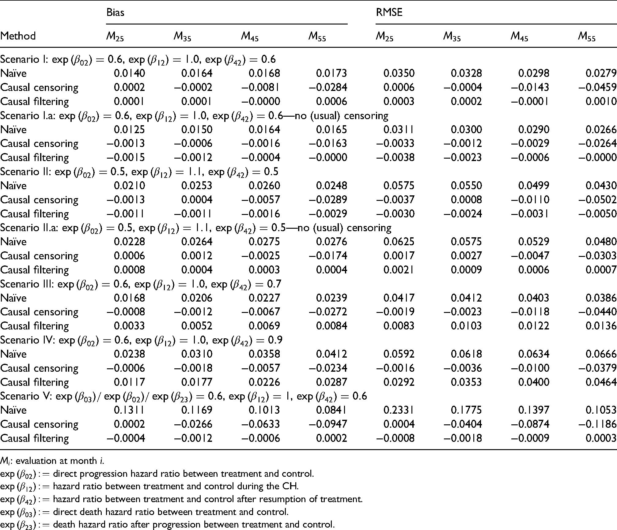
We simulate different scenarios (ID I–IV) where the treatment effect of the OS is manifested primarily in a treatment effect on the time until progression. Compared to the original START trial, we focus on a more considerable treatment effect. We consider a direct progression hazard ratio between treatment and control of 0.6 in all scenarios, except in Scenario II, where we consider an even more pronounced treatment effect of 0.5. For Scenario I.a and Scenario II.a no censoring times are simulated. That means all censored observations are due to the CH. Scenarios III and IV treat the case where the treatment effect is not restored. Transition hazards that are not manipulated within a scenario are parametrically estimated from the START data.
Additionally, we consider a scenario (ID V) that deviates more from the original START setting, but shows a larger negative impact of the CH.
We simulate 1000 studies with a sample size of 1500 individuals assigned in a 2:1 ratio to the treatment or control group. Random censoring times are generated from a Gompertz distribution for all patients, which roughly mimicked the empirical censoring distribution in the original data.
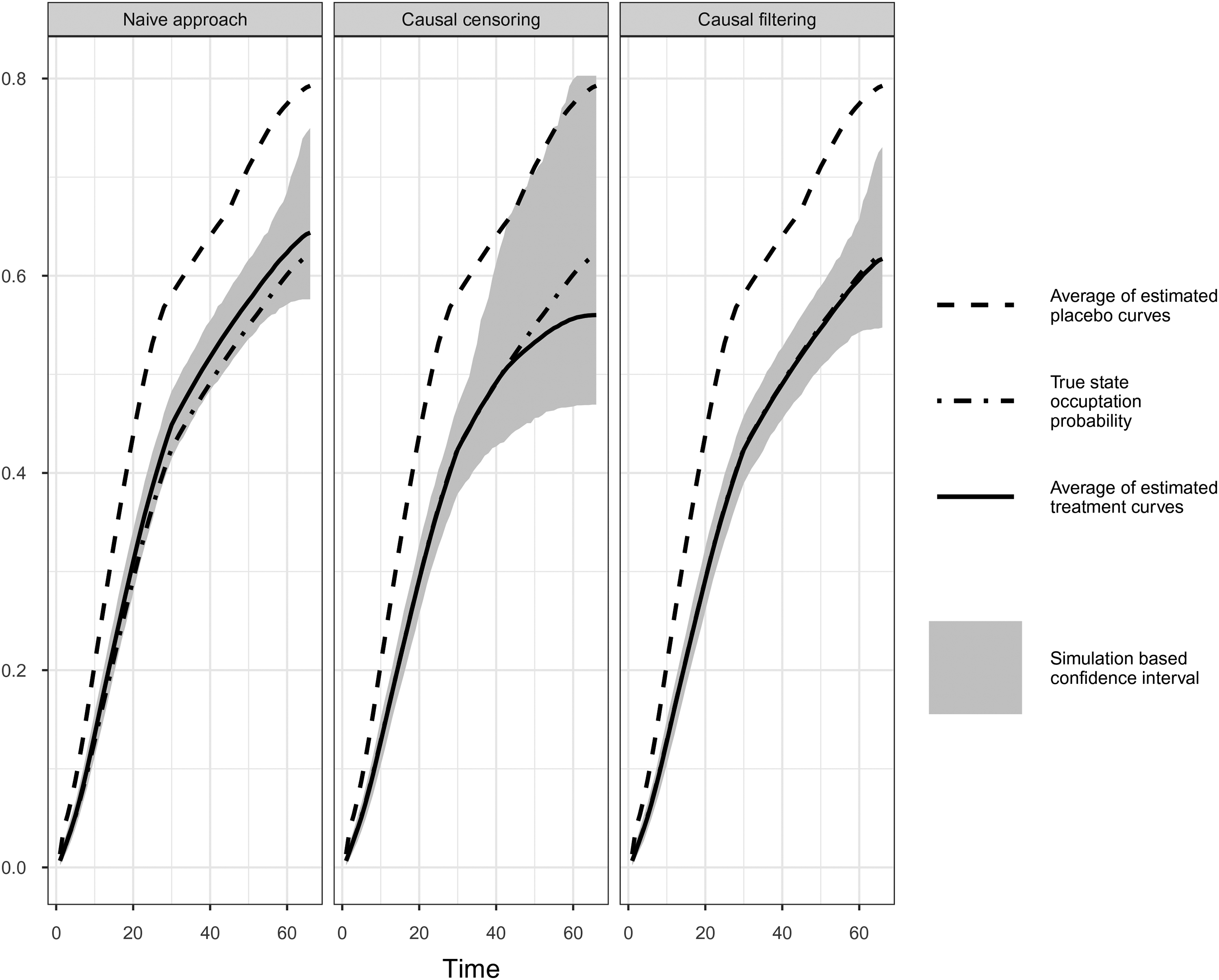
To show whether our causal censoring and filtering methods (i.e. “censoring by treatment interruption” and “filtering by treatment interruption,” cf. Section 3.3.) provide causal estimates under “do(no CH)” we compare Aalen-Johansen estimates averaged over 1000 simulation iterations with the true averaged Aalen-Johansen estimator in the absence of CH. As we are interested in the treatment effect of OS we consider the state occupation probability of “death,”
Table 2 shows the bias and the root mean squared error (RMSE) of the Aalen-Johansen estimates at different months for the different treatment effects. Table 3 presents averaged estimates of the time-varying relative risks for the same scenarios and selected time-points. Figures 7 to 9 report the average of the 1000 estimates of
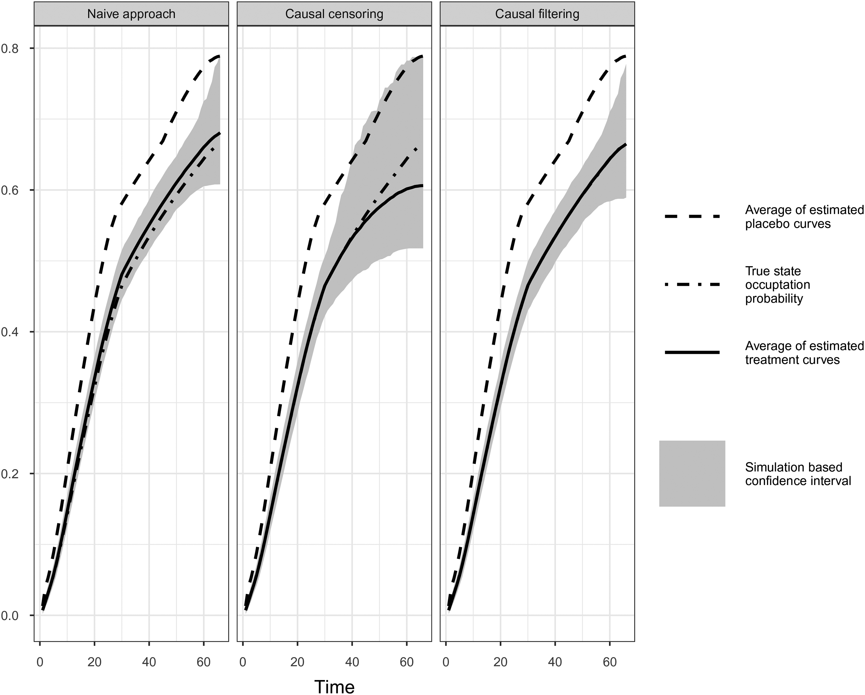
Comparison of simulation results of naïve, causal censoring and causal filtering approach. Simulation scenario I:
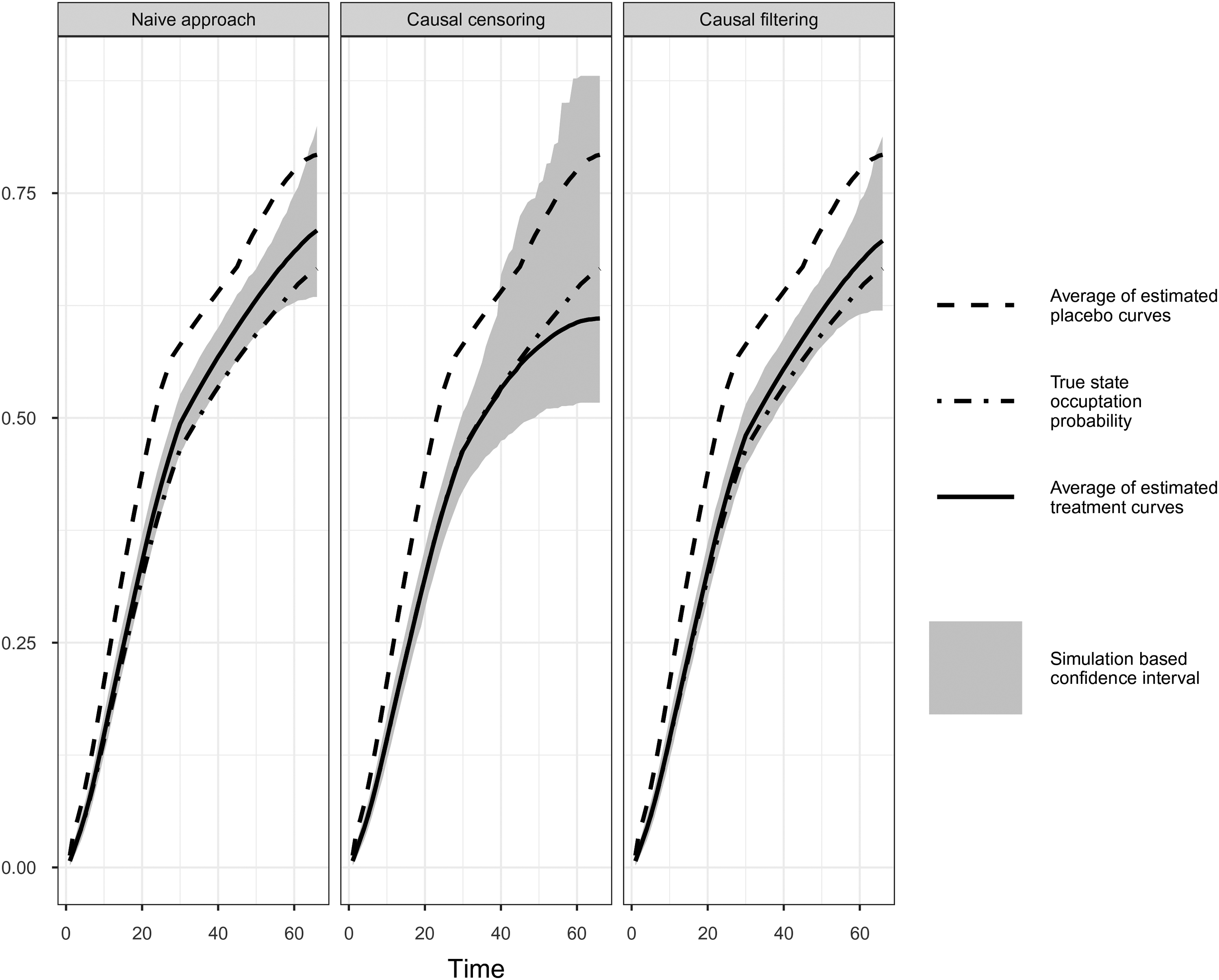
Comparison of simulation results of naïve, causal censoring and causal filtering approach. Simulation Scenario II:
Comparison of simulation results of naïve, causal censoring and causal filtering approach. Simulation Scenario IV:
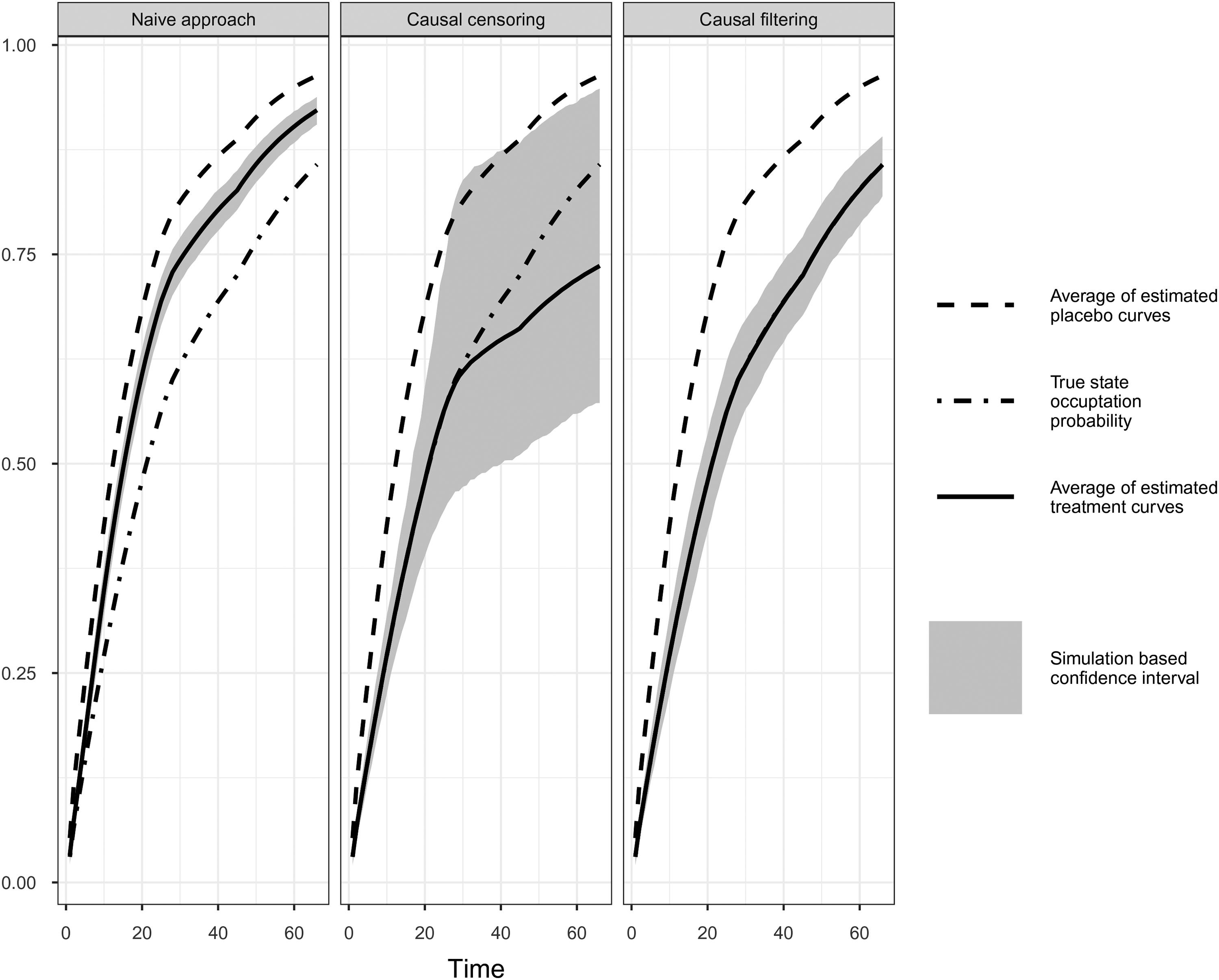
Comparison of simulation results of naïve, causal censoring and causal filtering approach. Simulation Scenario V.
Causal censoring and filtering approaches compared to naïve approach: Bias and root mean squared error (RMSE) of averaged Aalen-Johansen estimates of
Causal censoring and filtering approaches compared to naïve approach: Average of estimated time-varying relative risks including bias and root mean squared error (RMSE) at different and arbitrary time-points (in months from start of trial).

In the present article, we have pointed out that censoring or filtering the empirical transition matrix by treatment interruption induced by an external mechanism has a causal interpretation towards a treatment effect under do(no treatment interruption) using the example of the CH in the phase III START trial with the primary endpoint OS.
We suggested a censoring approach which censors all progression-free patients of the treatment group at the start of the CH and a filtering approach which restarts observation after the end of the CH. We showed that estimating the transition matrix after applying our censoring and filtering approaches can be seen as an implementation of the g-computation formula. We further discussed requirements on the censoring or filtering mechanism for drawing causal inference in the presence of a time-varying treatment. An important finding is that we do not necessarily need random censoring (or filtering), but rather the independent censoring (or filtering) assumption has to be fulfilled and, in addition, the state space of the multistate model has to be rich enough to justify a causal interpretation. In our example, if progression were not in the model, the treatment effect for OS would be subject to selection bias, as patients who are longer non-progressive are more likely to be censored. That means that all covariates that we need to produce conditional exchangeability, which is an essential assumption for the identification of causal effects, must be captured by the multistate model. Censoring by an external covariate ensures exchangeability. The crucial point here is the correct identification of the causal DAG and the specification of a suitable Markov model.
The two concepts independent censoring and exchangeability have in common that they claim that the individuals are representative in a certain way. Independent censoring implies that the observed individuals are “representative” of the incompletely observed individuals in the sense that the intensity of the counting process in the complete data world can be estimated. Exchangeability refers to the intervened individuals that are representative of the non-intervened individuals—had they been intervened—such that probabilities from a hypothetical world, where the intervention is active, can be estimated.
An example where independent censoring does not (generally) provide causal estimates is censoring by competing risks. Censoring by the competing event implies that censoring depends for each individual on the type of event that occurred. This kind of censoring is independent with regard to the identification of the hazard of the cause-specific event of interest. However, there will be (unmeasured/unknown) causal parents that affect both types of event. Consequently, we do not know whether the cause-specific hazards would alter in a world where one could only die from one cause of failure, if the competing risks are different causes of death. Moreover, we could (generally) not define a plausible and realistic intervention to remove the competing event. 25 Consequently, the effect of treatment on the event of interest in a world without competing event could not (generally) be identified from the observed data, as neither the consistency nor the exchangeability assumption is fulfilled. However, there might be situations where the competing event is nothing that inevitably has to happen, and, thus, a realistic intervention could be constructed. Transplantation as competing risk for dialysis patients is such an example. 26
In simulation studies, we compared the naïve approach, which simply ignores the CH, with a causal censoring and a filtering approach for different scenarios. We found that both approaches provide causal estimates of the treatment effect which would had been observed in the absence of the CH. Under the additional assumption of the treatment effect being restored after lifting the CH, the filtering approach is preferable as it incorporates the fact that most of the patients resume treatment after the CH. Thus, filtering leads to more observed event times and, especially at late time-points, the estimates of the transition probabilities using filtering are more accurate and the simulation-based CIs are smaller provided that the treatment effect is more or less restored after the end of the CH. This assumption can be checked, for instance, by comparing the Nelson-Aalen estimates before and after the treatment interruption due to the CH. In terms of statistical inference, the standard asymptotic results and mathematical arguments for counting processes 15 can be applied to our censoring and filtering approaches, under the assumption of censoring or filtering being independent. Moreover, bootstrap techniques are applicable and are a convenient approach for constructing confidence intervals.27,28However, the Aalen-Johansen estimates as well as the relative risks that we have considered in the simulations studies are determined at specified time-points. A line of future research would be to provide a single estimate for the contrast between control and treatment groups including confidence intervals and p-values. An option might be to use restricted mean survival time (RMST) analysis, Royston and Parmar,e.g. 29 which has the advantage that it can deal with non-proportional hazards. Estimation of the RMST is straightforward using the Aalen-Johansen estimator and allows the application of re-sampling methods like the wild bootstrap 30 that also applies in non i.i.d. scenarios like event-driven trials.31,32 Another possibility would be the multistate resampling method proposed in Bluhmki et al. 33 that uses Nelson-Aalen estimates to generate bootstrap data sets from which we could derive bootstrapped hazard ratios. The trick here is that the method of Bluhmki et al. 33 allows to generate synthetic bootstrap data sets after causal censoring or filtering.
In addition to the censoring and filtering approaches, we performed an analysis of a treatment effect in the absence of CH using the popular structural accelerated failure time model (SAFTM). Theoretical considerations and the simulation results are included in the Supplemental Materials. The SAFTM also makes a number of strong assumptions. Besides the assumptions of rank-preservation and “no unmeasured confounders,” an equal treatment effect for patients switching to treatment as for those who initially receive the treatment is assumed. In contrast to our non-parametric censoring approach, the SAFTM assumes a parametric and deterministic relationship between the counterfactual event times and the observed event times. Compared to the naïve approach, the SAFTM reduced the bias induced by the treatment interruption considerably in our analyses. As measured by the derived hazard ratios, the results of the SAFTM are comparable, but not better than the results of our proposed censoring and filtering approaches.
The considerations within this paper also considerably extend earlier investigations of Nießl et al., 2 who proposed a multistate model incorporating the CH, analyzed the impact of the CH, and suggested several methods to account for its impact, including a causal censoring approach that censors all patients at the start of the CH regardless of treatment group and progression status. However, Nießl et al. 2 did not provide a formal and general argumentation. One advantage of the censoring and filtering approaches considered in the present article is that the number of observed events included in the analysis is much higher confirming that the understanding of the causal relations might help to improve the analysis strategy. In the Supplemental Materials, the censoring approach that censors all patients (see “Censoring by CH” in Section 3.3.) and the mITT analysis, as applied to the START study and as described in Nießl et al., are applied to the simulated scenarios I to IV and compared with our censoring and filtering approaches. Overall, we can state that the mITT analysis leads to a small bias for all time points. The censoring method is unbiased for early time points, but shows a large bias for later time points (the bias is larger than for the causal censoring approach), which can be explained by the smaller number of observed events compared to the other methods.
We also applied our new methods to the original START trial (results not shown). Until month 30 we see hardly no differences between the Aalen-Johansen estimates of mITT, naïve and the causal method and only a moderate treatment effect. This is in line with previous analyses.1,2 After month 30, the causal censoring method approaches more clearly the placebo curve compared to the other methods, which is probably due to the small number of events, as also observed in the simulations.
As Nießl et al., 2 we assumed that our multistate model fulfills the Markov assumption common in causal reasoning, 18 which is a strong assumption. This implies that we assume that progressive patients have the same risk to die regardless of whether they have experienced the CH or not in the past. An alternative would be to consider a semi-Markov model, in which the post-progression hazard depends on the time since progression. However, censoring on the post-progression time scale will lead to dependent censoring in a non-Markov model and conditioning on an intercurrent event will not lead to a causal analysis. Another alternative is to model the post-progression hazards with time to progression as a covariate. Overall, it is a topic of future research to discuss the possibilities and implications of causal censoring also for non-Markov settings, the latter being an active field of research for ‘standard’ (not necessarily causal) multistate models. 31
Another interesting point for future research are causal censoring approaches in the presence of interval-censored data. Interval censoring implies that the occurrence of an event is only known to fall in some time interval, but the exact event time is not known. We refer to Chen et al. 34 for general methods for interval-censored data including an application for estimating a causal effect in the presence of interval-censored data. The connection to our motivating trial is that occurrence of progression is typically interval censored. Hence, our intermediate state has to be interpreted as progression diagnosis, which is not interval censored. It is progression diagnosis that informs treatment interruption or start of a second line treatment.
Our developments allow to apply causal censoring or filtering in general settings with externally induced non-adherence to the study protocol. For example, one possible application of the causal censoring would be to answer the question: What would be the treatment effect of a clinical trial in the absence of COVID-19? The pandemic has caused many direct and indirect effects affecting the planned conduct of a clinical trial. The time of censoring could be a defined anchor date indicating the start of indirect impact of the pandemic. 7
Supplemental Material
sj-pdf-1-smm-10.1177_09622802221133551 - Supplemental material for A connection between survival multistate models and causal inference for external treatment interruptions
Supplemental material, sj-pdf-1-smm-10.1177_09622802221133551 for A connection between survival multistate models and causal inference for external treatment interruptions by Alexandra Erdmann, Anja Loos and Jan Beyersmann in Statistical Methods in Medical Research
Supplemental Material
sj-r-2-smm-10.1177_09622802221133551 - Supplemental material for A connection between survival multistate models and causal inference for external treatment interruptions
Supplemental material, sj-r-2-smm-10.1177_09622802221133551 for A connection between survival multistate models and causal inference for external treatment interruptions by Alexandra Erdmann, Anja Loos and Jan Beyersmann in Statistical Methods in Medical Research
Footnotes
Declaration of conflicting interests
The author(s) declared no potential conflicts of interest with respect to the research, authorship and/or publication of this article.
Funding
The author(s) disclosed receipt of the following financial support for the research, authorship, and/or publication of this article: Jan Beyersmann was partially supported by German Research Foundation (DFG) grant BE 4500/4-1.
Supplemental material
Supplemental material for this article is available online.
References
Supplementary Material
Please find the following supplemental material available below.
For Open Access articles published under a Creative Commons License, all supplemental material carries the same license as the article it is associated with.
For non-Open Access articles published, all supplemental material carries a non-exclusive license, and permission requests for re-use of supplemental material or any part of supplemental material shall be sent directly to the copyright owner as specified in the copyright notice associated with the article.