
Abstract
We revisit several conditionally formulated Gaussian Markov random fields, known as the intrinsic conditional autoregressive model, the proper conditional autoregressive model, and the Leroux et al. conditional autoregressive model, as well as convolution models such as the well known Besag, York and Mollie model, its (adaptive) re-parameterization, and its scaled alternatives, for their roles of modelling underlying spatial risks in Bayesian disease mapping. Analytic and simulation studies, with graphic visualizations, and disease mapping case studies, present insights and critique on these models for their nature and capacities in characterizing spatial dependencies, local influences, and spatial covariance and correlation functions, and in facilitating stabilized and efficient posterior risk prediction and inference. It is illustrated that these models are Gaussian (Markov) random fields of different spatial dependence, local influence, and (covariance) correlation functions and can play different and complementary roles in Bayesian disease mapping applications.
Keywords
Introduction
In the Bayesian disease mapping literature, several conditionally formulated Gaussian Markov random fields (GMRF), also known as conditional autoregressive (CAR) models, have been proposed as spatial prior options for random effects in spatial generalized linear mixed effects (GLMM) models for spatially aggregated areal data. 1 For mapping disease risks in small geographic areas, Bayesian GLMM Poisson models are typically used, in which the random effects represent log relative risks for geographic areas under study, e.g., counties or local health areas of a province or state or country; see Lawson 2 and Martinez-Beneito and Botella-Rocamora. 3 The present paper concerns with mapping of a single disease, for which the main goals are typically to ascertain geographical risk distribution of the disease and identify geographic areas of elevated (and lowered) disease risks. To achieve these goals, hierarchically formulated Bayesian GLMM is commonly used to model disease incidence or mortality data and to facilitate stabilized and efficient posterior risk prediction and inference.
Without essential loss of generality, we consider a typical disease mapping model, a hierarchically formulated Bayesian GLMM of Poisson likelihood for areal data of observed disease incidence or mortality cases, denoted


In MacNab, 6 the three CARs, and the BYM and MBYM, were studied together as prior options in Bayesian disease mapping. The present study revisits and extends the topic by researching these models analytically, via graphic visualization, and with comprehensive simulation and case studies. The main objective, contribution, and message of the present paper is to shed light on the risk models discussed herein, not just as competing prior options for spatial smoothing but also as complementary risk models in disease mapping, spatial regression, and related studies. We do so by presenting important insights and critique on these models for their nature and capacities in modelling spatial dependencies, local influences, spatial correlations, and spatially structured heterogeneities, and in facilitating stabilized and efficient posterior risks prediction and inference based on data of extremely rare or rare or more common disease.
Another contribution of the present study is the illustration of a recent proposal of deviance information criterion (DIC12,9–11) and the widely applicable information criterion (WAIC13–15) for model evaluation and comparison via simulation and case studies. In addition, a new proposal of adaptive MBYM is put forward and illustrated in Bayesian disease mapping and spatial regression.
The rest of the paper is organized as follows. Section 2 reviews the above-mentioned risk models analytically and via graphical illustrations. Section 3 presents a comprehensive simulation study that further elucidates the risk models and associated Bayesian method for posterior estimation and inference. Section 4 presents the three case studies illustrating Bayesian disease mapping based on data of extremely small, small, modest, and large sample size, respectively. Section 5 concludes with a summary discussion.
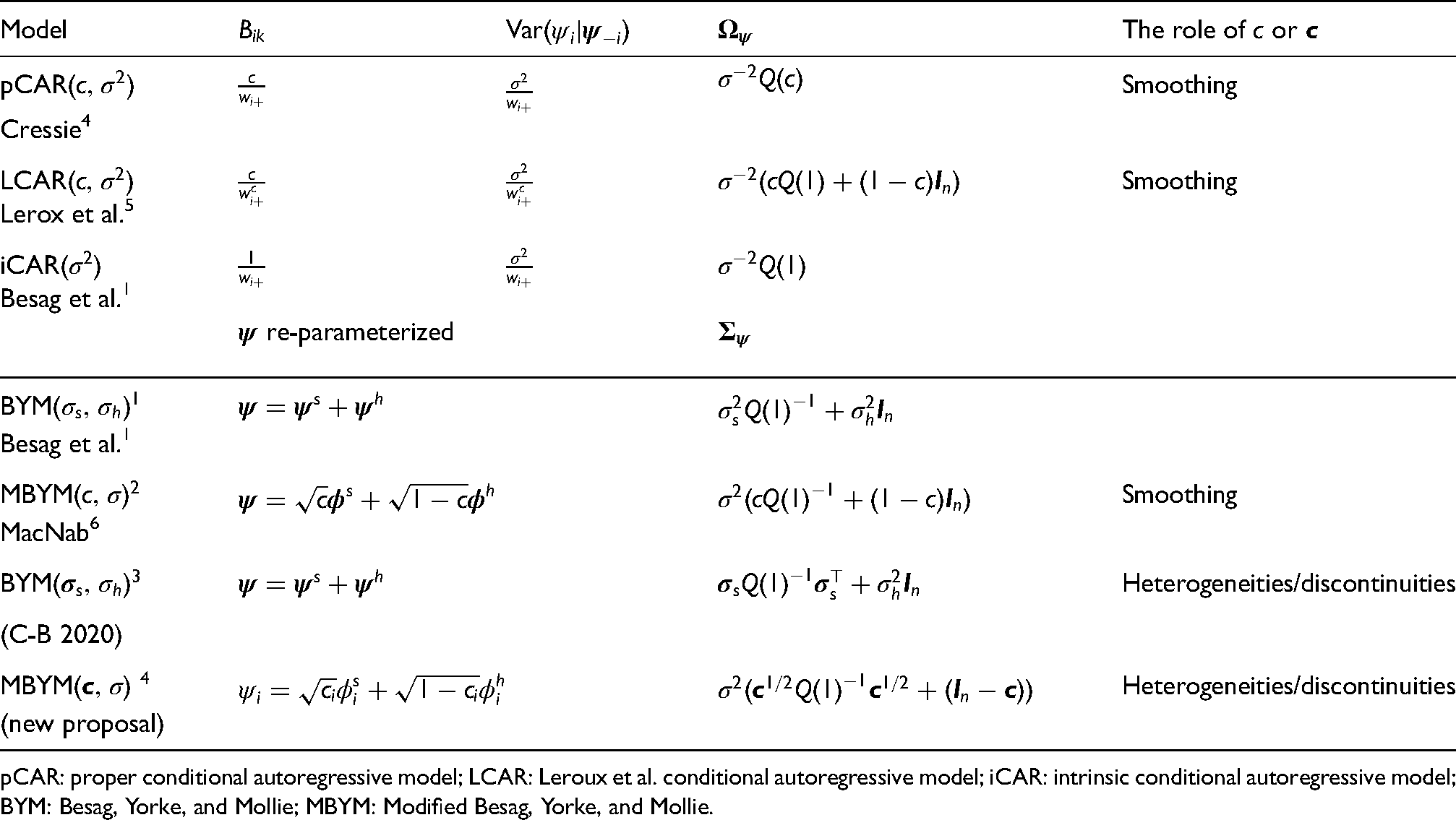
A CAR construction and its three options of parameterization
The following Gaussian conditional mean and variance functions define a general construction of CARs:


GMRFs are undirected graphical models that characterize probabilistic interactions of directly related variables.6,17 Of the GMRFs commonly used in disease mapping (see Table 1), the
Options of model parameterization.
pCAR: proper conditional autoregressive model; LCAR: Leroux et al. conditional autoregressive model; iCAR: intrinsic conditional autoregressive model; BYM: Besag, Yorke, and Mollie; MBYM: Modified Besag, Yorke, and Mollie.
The GMRF precision matrix (6) must be symmetric and non-negative definite. To fulfil the two requirements, functional characterizations and simplified parameterizations to the CAR conditionals have been proposed (mainly) in the disease mapping literature; and the previously mentioned iCAR, pCAR, and LCAR are the most commonly used GMRFs in disease mapping applications at the present time; see Table 1 for the CAR specifications, where key references are given. The three CAR formulations and parameterizations are commonly viewed as competing spatial risk priors; each has its strength and limitations, which we discuss and illustrate in this section.
The CARs were initially proposed to facilitate borrowing information and spatial smoothing.1,4,5 However, shown in MacNab, 18 and in the present paper, as we broaden the scope of Bayesian disease mapping to the studies of rare or more common diseases, and non-communicable or communicable diseases, CARs and GMRFs can offer tools not just for borrowing information and spatial smoothing, but for analysis of spatial risk dependencies, local risk influences, spatial risk correlations, and spatial risk heterogeneities.
The pCAR(
pCAR
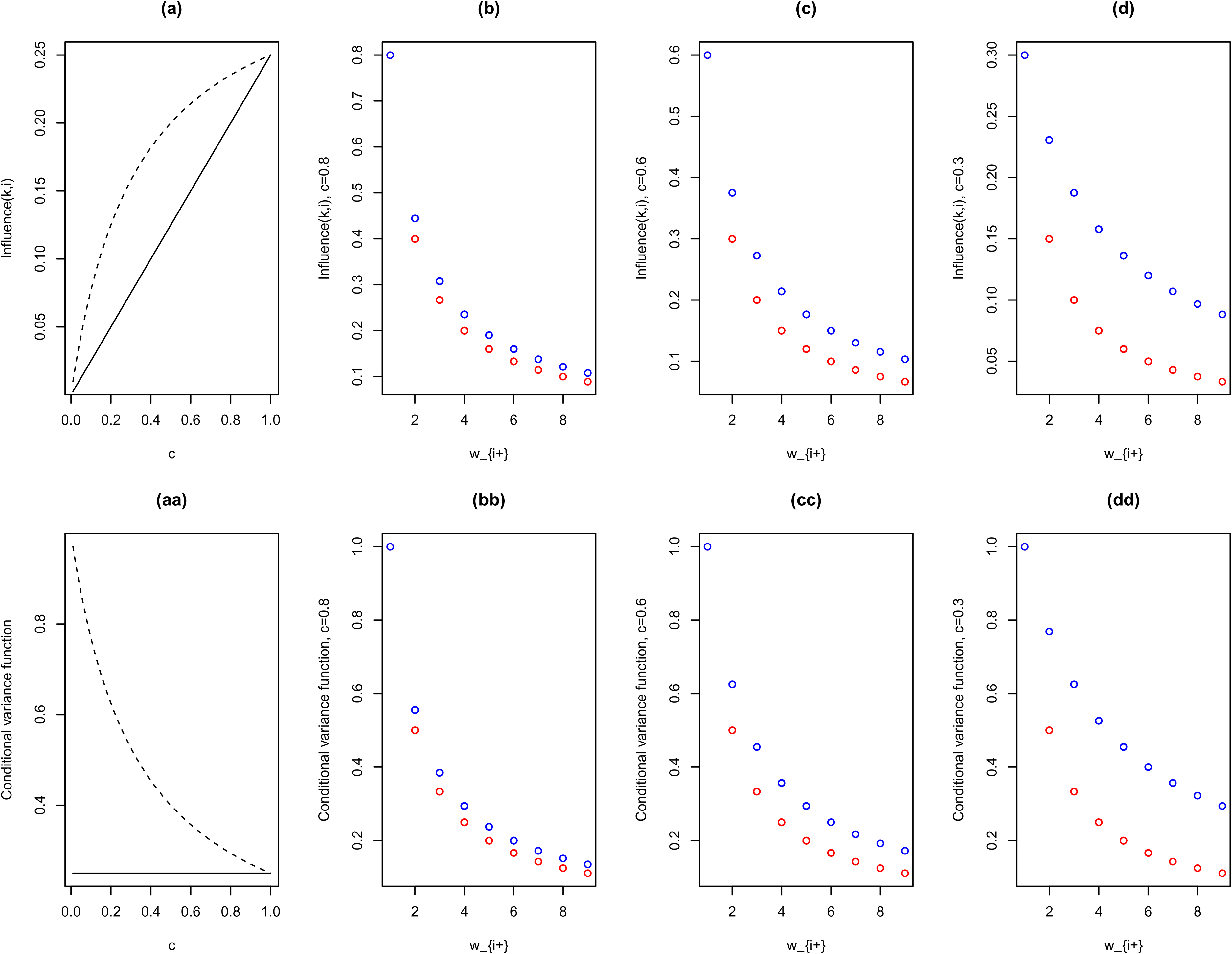
As Figure 1 illustrates, the pCAR influence function, Influence
In Bayesian disease mapping, the spatial parameter
In LCAR, the spatial dependence parameter
The LCAR is often favoured over the pCAR for the fact that, when
The scale parameter
The one-parameter iCAR(
In disease mapping, the iCAR (7) is commonly used when the
In the present paper, we illustrate that, to gain identification, posterior estimation and inference of BYM can be implemented by placing (weakly) informative priors on the BYM scale parameters or by a reparameterization of BYM, named modified BYM or MBYM in MacNab
6
:
While not discussed in the literature, in the present paper we also highlight and critique on the re-parameterization approach to identification by noting that it is equivalent to placing functional constraints on the BYM scale parameters
A scaled iCAR(
The CAR conditionals (5), and the resulting sparse precision matrix
However, some of the characteristics of the GMRF covariance matrices, as well as the (M)BYM covariance matrices, can be explored and understood by graphic visualization, such as plots of spatial correlation and covariance functions, as well as the marginal variance functions, for given model parameters. Here, we define spatial correlation or covariance functions as correlation
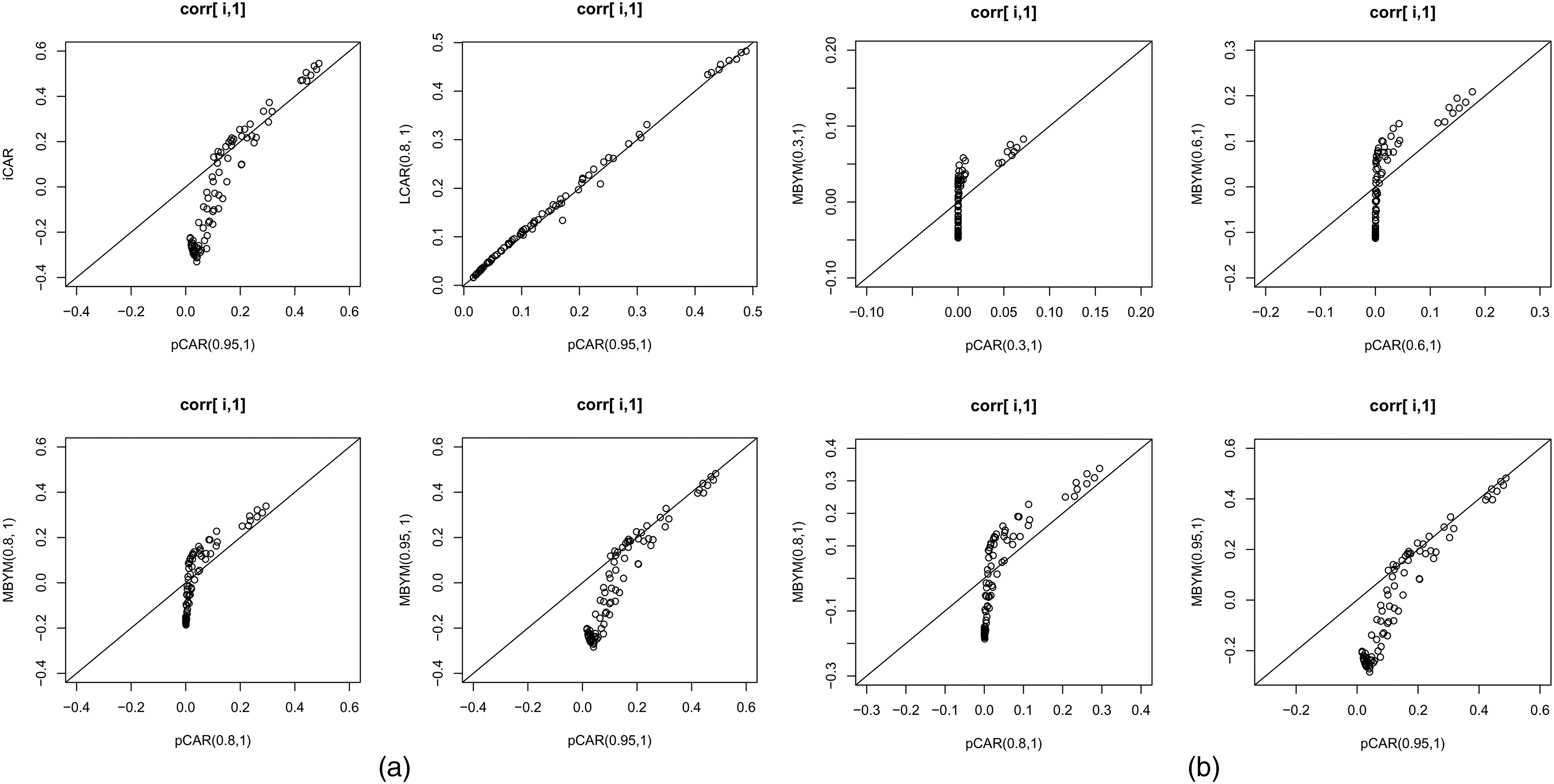
Illustrative spatial correlation functions for the pCAR, LCAR, iCAR and MBYM, respectively, with indicated parameter values. The spatial correlation functions display correlations between county 1 and county
Specifically, for iCAR, pCAR, LCAR and (M)BYM, Figure 2, and the supplement Figures S1 and S2 display spatial correlation functions between county 1 and county
Illustrated in the supplement Figure S1, even for small values of spatial parameters, the pCAR and LCAR model locally clustered spatial correlation functions. It also shows that the differences between pCAR and LCAR correlation functions are consistent with the differences in their influence functions (see Figure 1). For
In addition, the supplement Figures S1 and S2 illustrate that the iCAR and (M)BYM (of first-order adjacency-defined neighbourhood map) lead to positive and clustered spatial (correlation) covariances between an area and its first-order neighbours but negative (correlations) covariances between an area and its ‘distance’
Further more, the supplement Figure S2 offers new insight into the (M)BYM partial corrrelation functions: They are spatially varying functions that lead to locally clustered partial correlations when the spatially structure variation exceed the unstructured variation (e.g.
To allow for more flexible characterizations of spatial dependencies, local influences, and spatial heterogeneities/discontinuities, extensions of the CARs to adaptive spatial dependence parameterizations (
In the context of Bayesian disease mapping, an adaptive BYM, defined by iCAR(
Here, we propose and illustrate (via a case study) an adaptive MBYM(
The simulation study
We carried out a comprehensive simulation study in the context of hierarchical Bayesian estimation, learning, and inference of GLMM (1)–(4), for options of the non-adaptive CAR or convolution risk models as random effects prior. Posteriors of all unknowns were estimated via Markov chain Monte Carlo (MCMC) simulations implemented in
The simulation and computational details are presented in the Supplemental Material (SM) to the paper. Simulated data were generated to represent disease mapping scenarios of extremely small, small, modest, or large sample sizes (as of expected disease counts, see SM for details). Detailed results are also presented in the SM, including seven tables (named the supplement Tables S1 to S7) and 14 figures (named the supplement Figures S3 to S16). Here, the key results are summarized and highlighted. The overall performances of posterior estimation and inference of model parameters and relative risks (and
Overall, the pCAR, LCAR and (scaled) MBYM led to comparable performances in terms of posterior estimation of the spatial dependence or weight parameter: Under non-informative prior
For all simulation scenarios, the iCAR scale parameter was estimated with near-zero posterior bias and near-the-target coverage rate.
Consistent and comparable performances were observed from the posterior estimates of the (M)BYM and scaled (M)BYM model parameters. The (scaled) BYM was shown to perform slightly better than the (scaled) MBYM, observed from modestly lower posterior bias and rmse from the (scaled) BYM; this is particularly evident for data of extremely small sample size, likely as a result that the spatial weight parameter in MBYM is typically underestimated for a large
Overall, the CAR and (M)BYM models led to consistent and comparable performances in terms of posterior risk prediction and inference; minor or modest differences were only observed for data of extremely small sample size. For all simulation scenarios, the iCAR performed well in terms of posterior risk prediction and inference. For all models and simulation scenarios, and even for extremely small sample size, the 95% credible intervals for the county-specific relative risks led to near or above 90% coverage rates.
For pCAR, LCAR and MBYM, minor or modest posterior risk sensitivities to spatial parameter prior options were mostly observed from the posterior risk standard deviations (posterior risk uncertainties) and the resulting posterior risk coverage rates; posterior risk biases and root mean square errors remained robust; informative spatial parameter priors led to reduced posterior risk standard deviations and improved posterior risk coverage rates.
In terms of posterior prediction and inference for relative risks (RRs) and the components
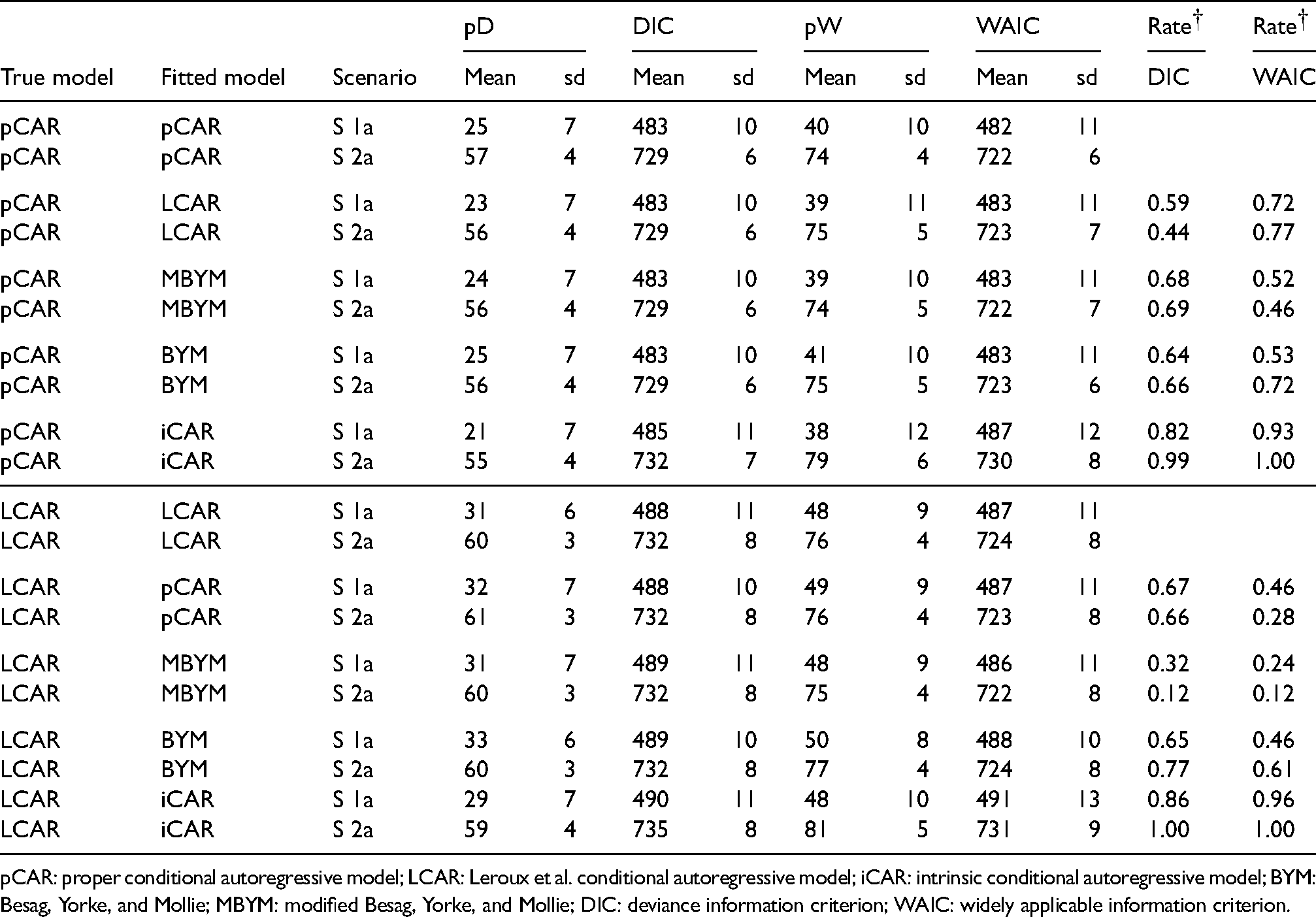
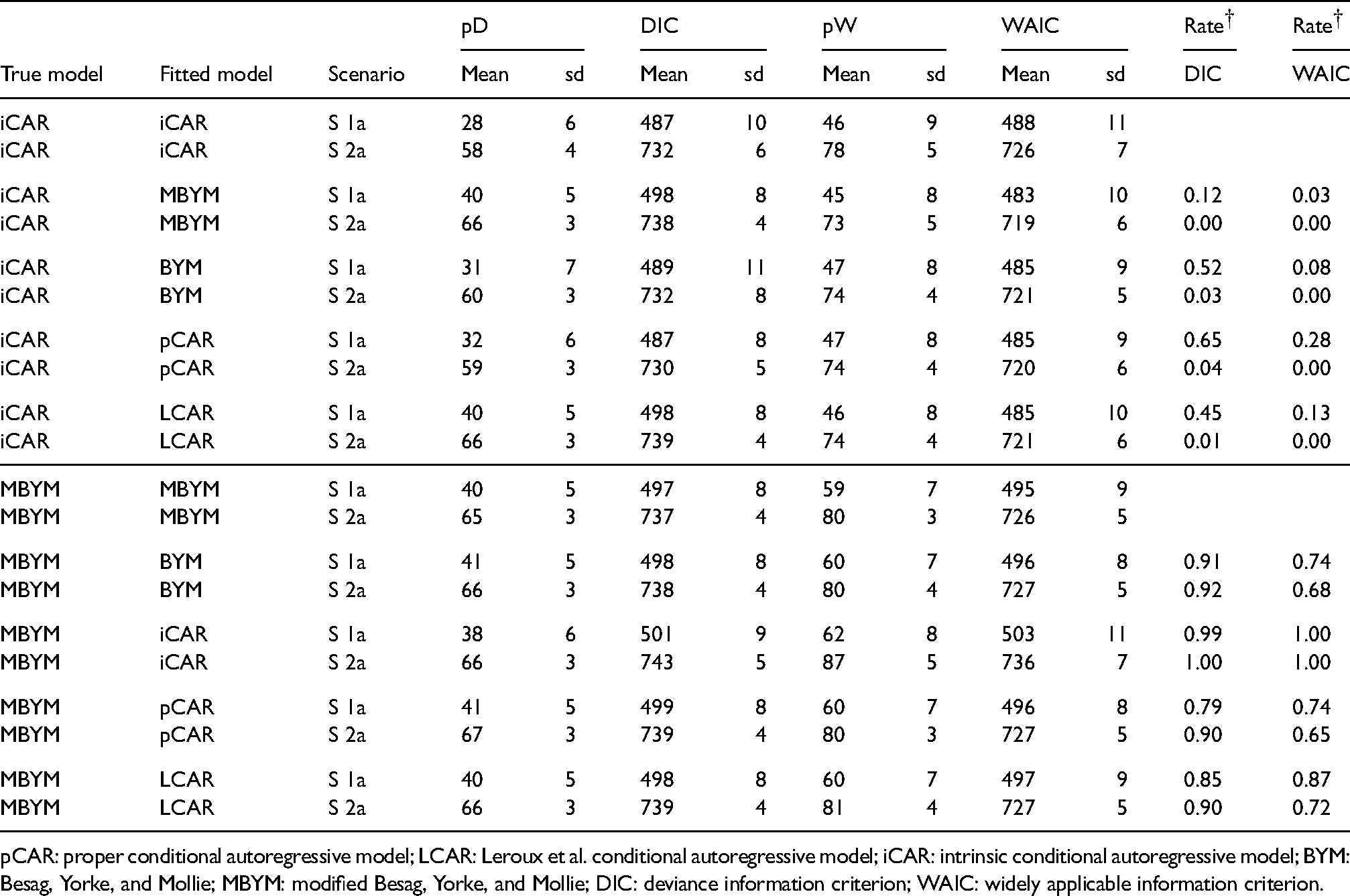
For the five risk models, we present here illustrative simulation results of deviance information criterion, the Dbar (deviance), pD, and DIC scores, where pD = pD1 and pD1 is the number of free parameters defined in MacNab,
10
in which the deviance, pD1 and DIC = Dbar+pD1 are invariant to re-parameterization and can facilitate model evaluation and comparison among (multivariate) CAR models, including those with non-identifiable or partially identifiable model parameter(s). Illustrative results of widely applicable information criterion (WAIC) were also presented, where WAIC = -2 lppd (predictive accuracy) +
The estimated DIC and WAIC statistics (e.g. mean scores and associated standard deviations) are overall comparable across the models, although the effective numbers of parameters in DIC (denoted pD) were consistently lower than those in WAIC (denoted pW); see Tables 2 and 3 and the supplement Figure S13 to S16 for illustrative results of simulation scenarios 1a and 2a. The two tables also present rates of true models preferred based on the estimated DIC and WAIC, respectively: The DIC-based rates may inform on model comparison in term of prediction accuracy of observed data (via deviance) and within-sample risk predictions, whereas the WAIC-based rates may inform on selection/comparison in term of out-of sample prediction accuracy (e.g. prediction accuracy of new counts and risks when new data is used).
Selected DIC and WAIC results of the simulation study (Part I),
for all models. Rate
: Rate of true model prefered based on the estimated DIC and WAIC, respectively.
Selected DIC and WAIC results of the simulation study (Part I),
pCAR: proper conditional autoregressive model; LCAR: Leroux et al. conditional autoregressive model; iCAR: intrinsic conditional autoregressive model; BYM: Besag, Yorke, and Mollie; MBYM: modified Besag, Yorke, and Mollie; DIC: deviance information criterion; WAIC: widely applicable information criterion.
Selected DIC and WAIC results of the simulation study (Part II),
pCAR: proper conditional autoregressive model; LCAR: Leroux et al. conditional autoregressive model; iCAR: intrinsic conditional autoregressive model; BYM: Besag, Yorke, and Mollie; MBYM: modified Besag, Yorke, and Mollie; DIC: deviance information criterion; WAIC: widely applicable information criterion.
Overall, when pCAR or LCAR or (M)BYM was the true risk model, the estimated DIC and WAIC scores led to consistent and high rates of favouring correct models when iCAR was the misspecified prior. When iCAR is the true risk models, the WAIC scores led to high rates of favouring pCAR, LCAR, and (M)BYM for both scenarios; this may suggest evidence that the iCAR is not a preferred out-of-sample predictive model among the five.
When the (M)BYM was the true data generating risk model, the DIC- and WAIC rates of true model preferred were consistent and comparably high (e.g. favouring the correct model), which suggested evidence that the (M)BYM may be a plausible risk model for both the within- and out-of-sample predictions.
The three case studies are presented herein to illustrate, via results of Bayesian GLMM (1)–(4), Bayesian risk mapping of extremely rare, rare, and more common diseases, represented by areal data of small, modest, or large (expected) counts (see Table 4 for summary statistics). The first case study was a re-analysis of the Jin et al.
28
cancer mortality data for 87 counties of Minnesota (USA). This data set contains county-level death counts (observed and expected) for cancer of oesophagus (
Data for the three illustrative case studies: Summary statistics of areal-level counts.
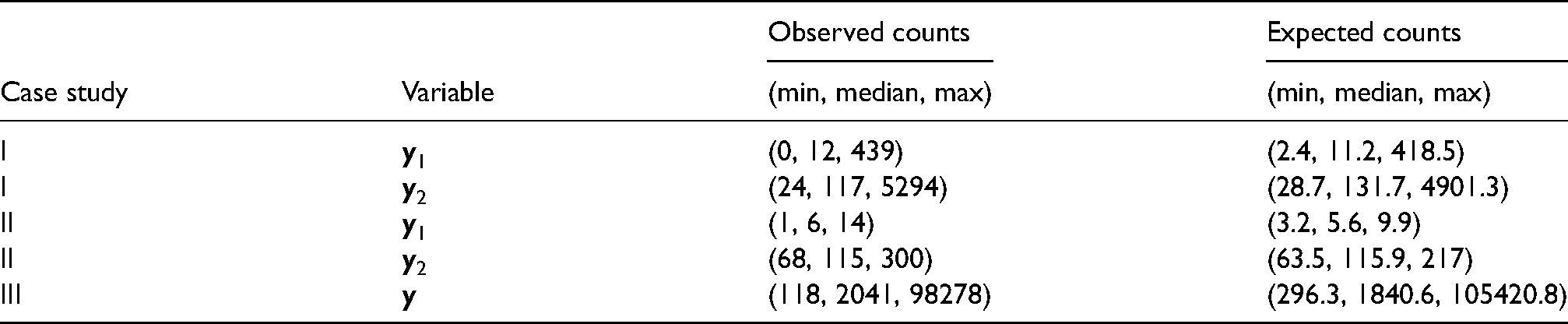
Data for the three illustrative case studies: Summary statistics of areal-level counts.
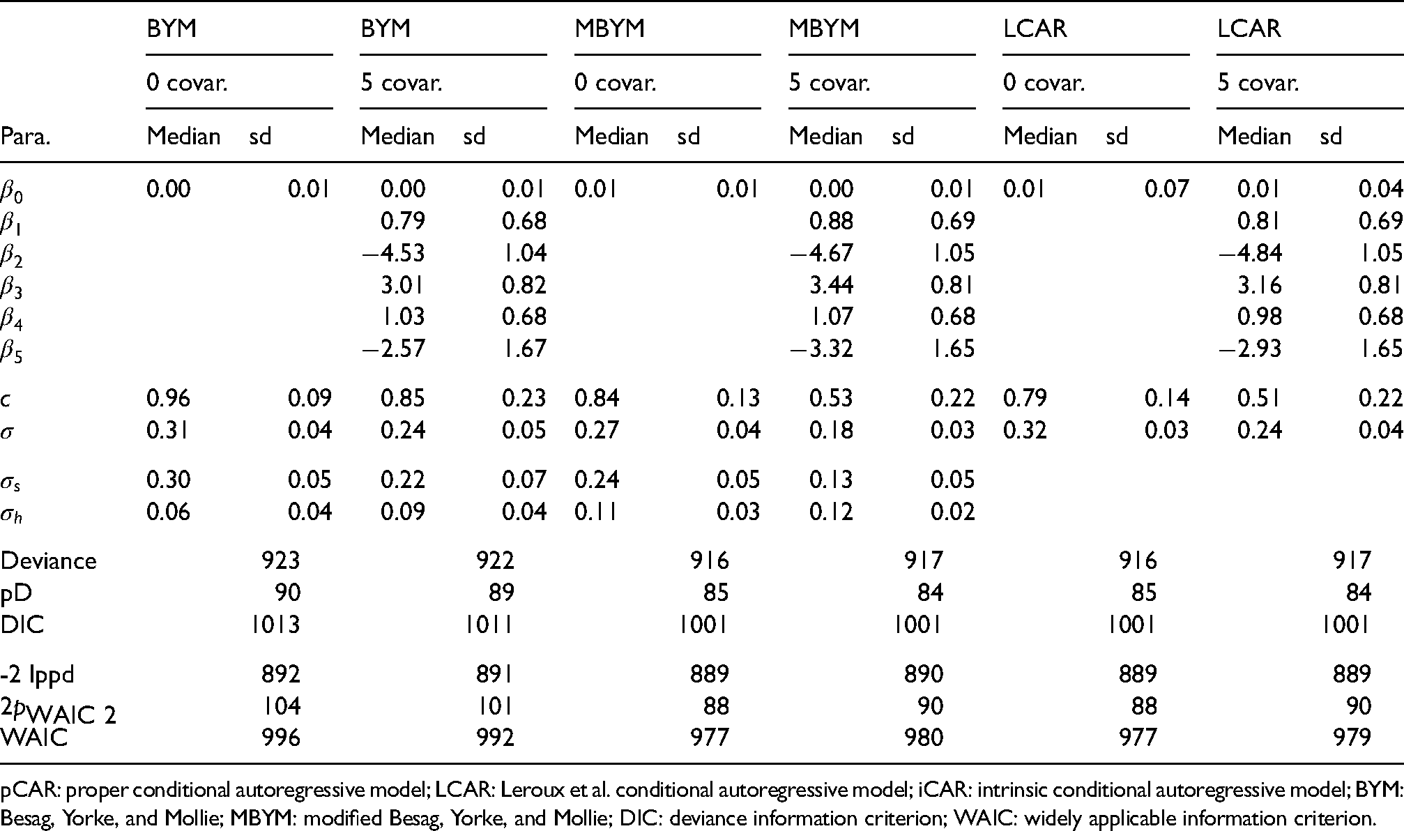
Posterior estimates (median and standard deviation) of the model parameters for all case studies are presented in the supplement Table S8, where modest to high spatial risk dependencies were suggested from the CAR models (indicated by modest to high posterior estimates of the spatial parameters). Consistent with the results of the simulation study, modest (although noteworthy) posterior sensitivities to spatial parameter prior specifications were observed from the first two case studies; Table 5 illustrates the results of pCAR. Modest posterior risk sensitivity was only observed from the case study II; Supplemental Figure S17 illustrates the results of pCAR.
Posterior estimates, median and standard deviation (sd), of model parameters under the indicated informative or non-informative hyperprior for
in pCAR(
).
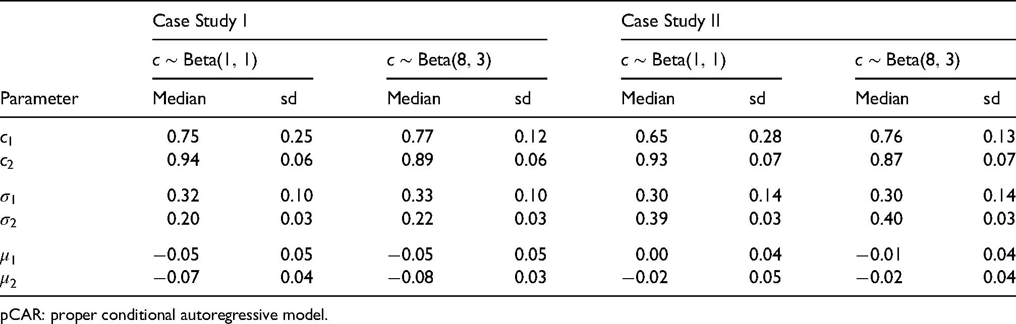
Posterior estimates, median and standard deviation (sd), of model parameters under the indicated informative or non-informative hyperprior for
pCAR: proper conditional autoregressive model.
Figure 3 illustrates comparable pCAR and LCAR posterior influence and predictive variance functions in the three case studies, calculated for the posterior medians of the spatial and scale parameters.
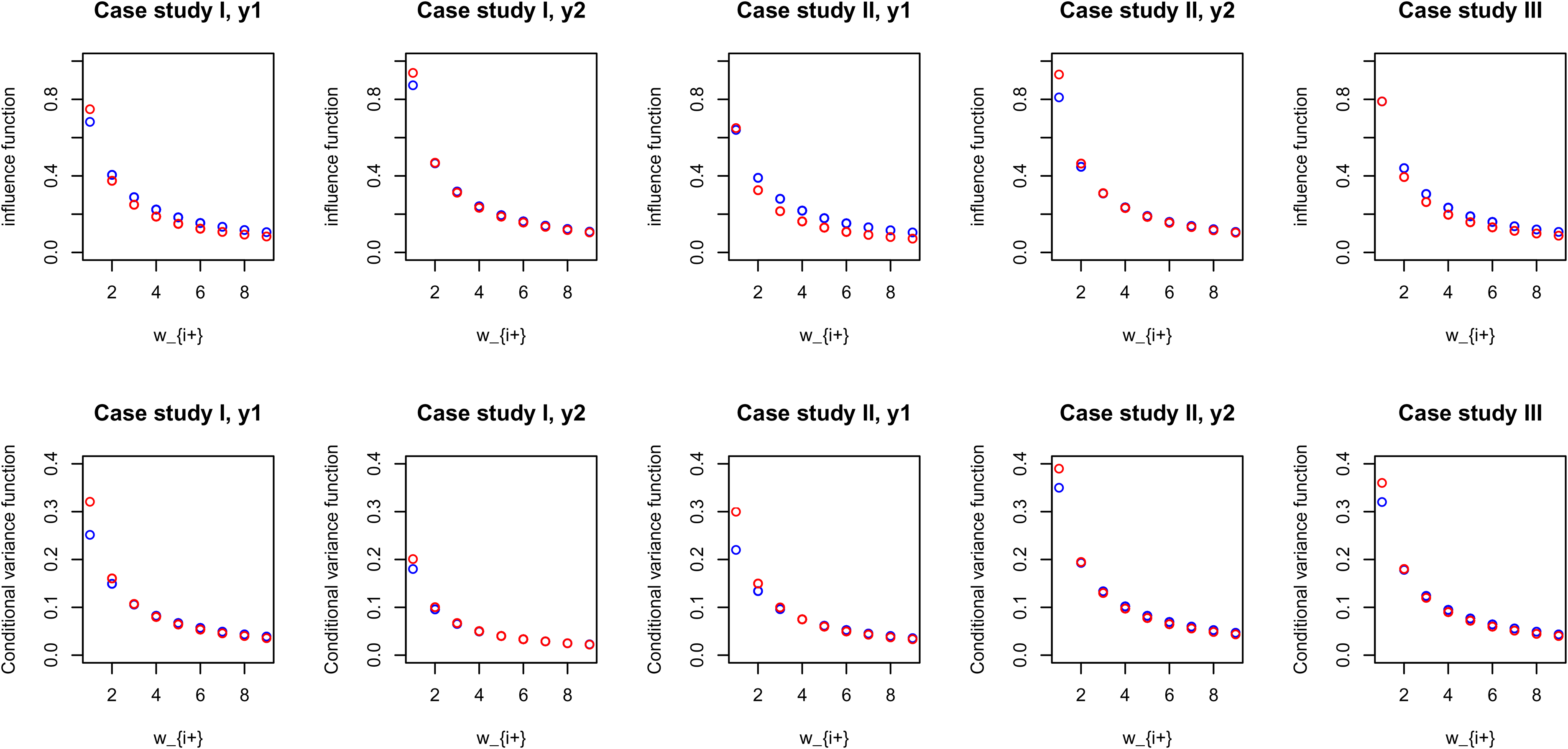
An illustrative comparison of estimated pCAR and LCAR posterior influence and conditional (predictive) variance functions for the three case studies, calculated for the posterior median of parameters
The DIC and WAIC results were overall consistent in each of the three case studies (see the supplement Tables S9 and S10). Of note is the DIC results for
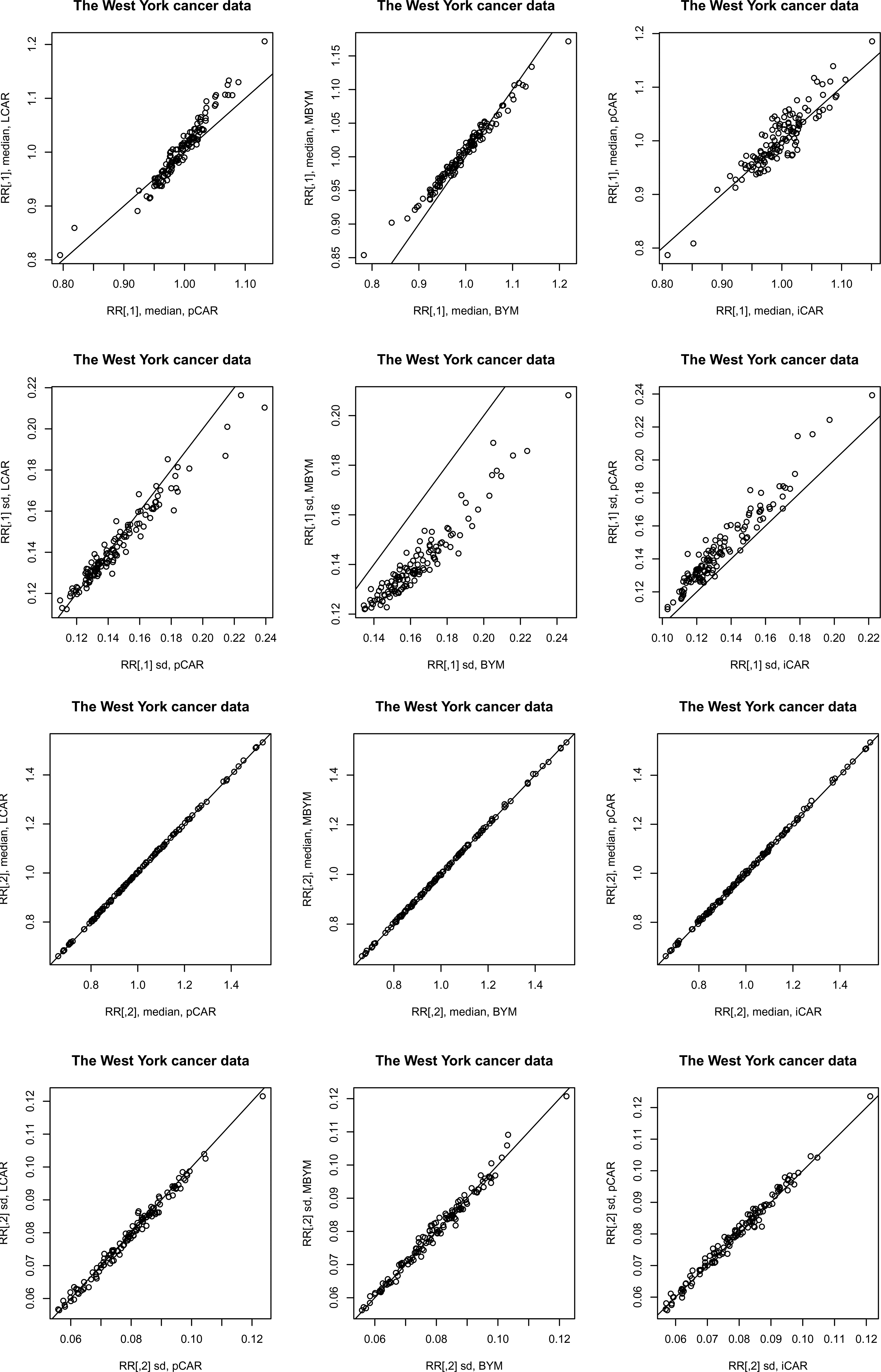
Posterior relative risk predictions for case study II: median – posterior median, sd – posterior standard deviation.
Results of the scaled iCAR and (M)BYM were also comparable to those of their unscaled counterparts. Figure 5 illustrates the results for (M)BYM of case study III; also see the supplement Tables S9 and S10 for DIC and WAIC results.
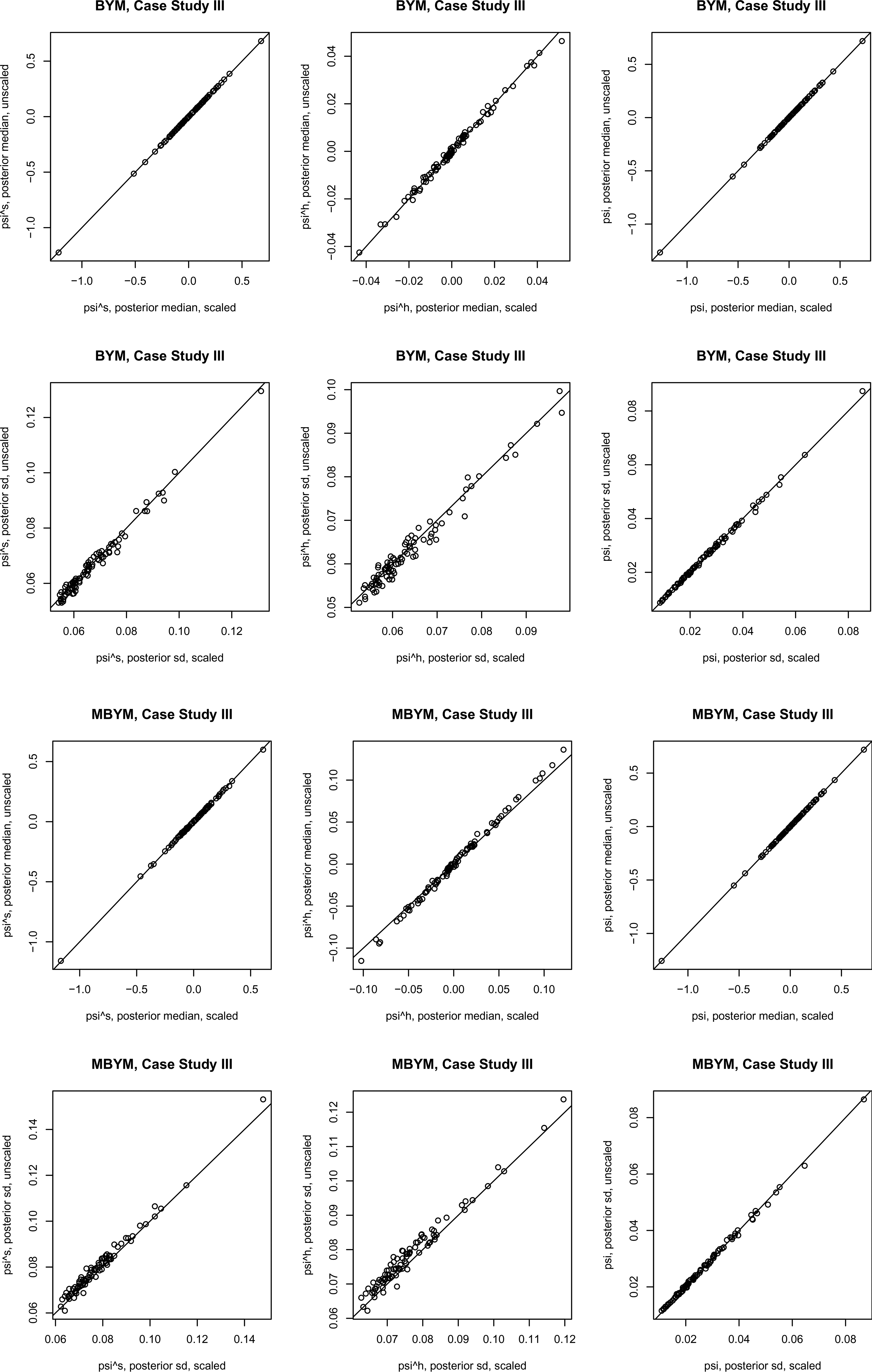
Posterior estimates, posterior median and standard deviation (sd), of the (M)BYM versus scaled (M)BYM
components
We present results of fitting the COVID-19 data to the spatial GLMM (1)–(4) without and with (five) covariates; see Table 6 for the names of the five covariates.
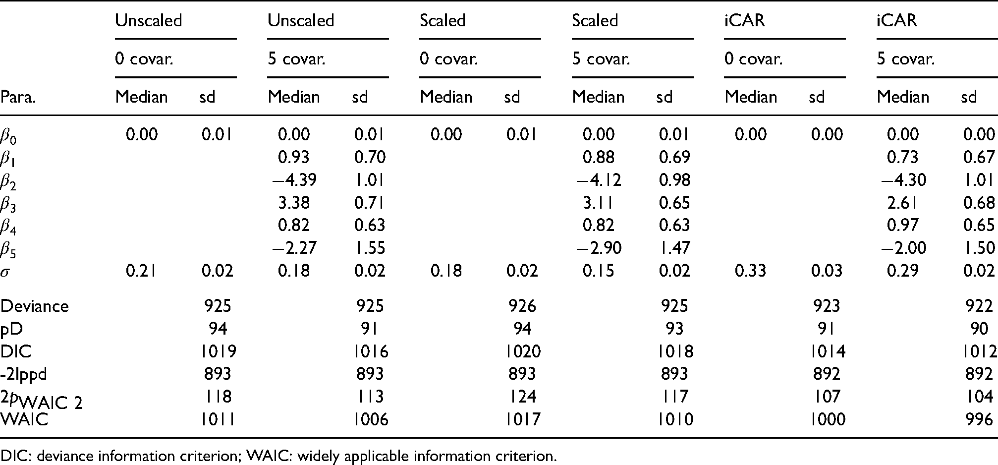
Posterior estimates, median and standard deviation (sd), of the model parameters without covariate (0 covar.) or with five covariates (5 covar.), for indicated priors. For BYM(
),
,
; for MBYM(
),
,
. The five covariates are scores of: Private transportation to work (
), Age 55–64 (
), Education less than high school (
), Colleage education (
), and Unemployment (
). The case study III.
Posterior estimates, median and standard deviation (sd), of the model parameters without covariate (0 covar.) or with five covariates (5 covar.), for indicated priors. For BYM(
pCAR: proper conditional autoregressive model; LCAR: Leroux et al. conditional autoregressive model; iCAR: intrinsic conditional autoregressive model; BYM: Besag, Yorke, and Mollie; MBYM: modified Besag, Yorke, and Mollie; DIC: deviance information criterion; WAIC: widely applicable information criterion.
Posterior estimates of the model parameters in spatial GLMM (1)–(4) without or with covariates are presented and compared in Table 6 and the supplement Table S11, where LCAR and pCAR outperformed the (scaled) (M)BYM with lower deviance (Dbar), pD and DIC scores. Consistent (but modest) reductions of the CAR spatial and scale parameter estimates from the GLMM without covariate to with covariates were observed (see Table 6 and Table S11), suggesting that the included covariates explained modest amounts of spatial risk dependence and risk variability (see the supplement Figure S20). The (scaled) MBYM, pCAR and LCAR risk models consistently suggested that the unexplained (residual) infection risks might be attributable to omitted covariates of spatially and randomly varying.
Figure 6 presents a comparison of posterior estimates of the (scaled) (M)BYM components of
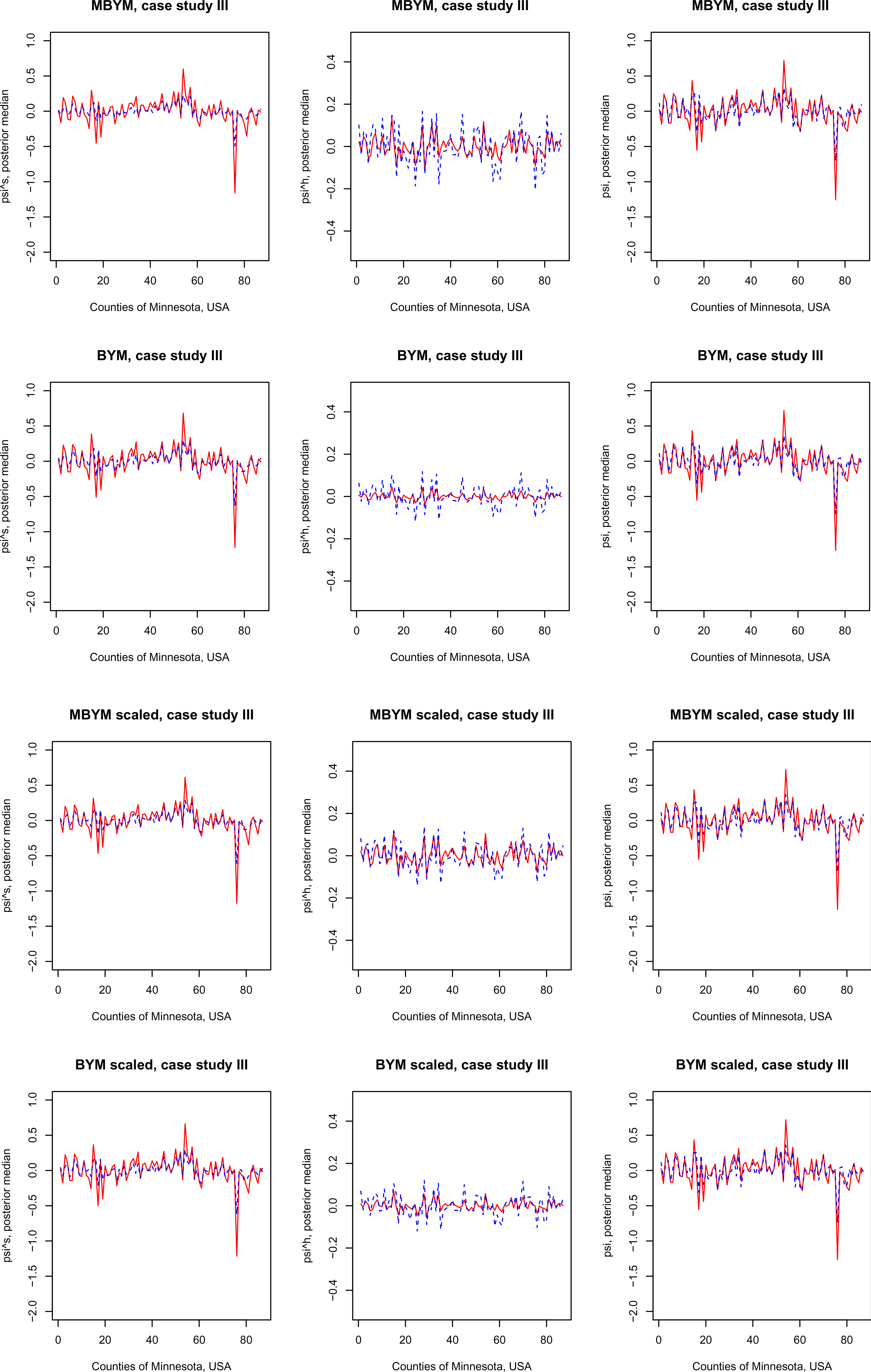
Posterior estimates, posterior median and standard deviation (sd), of the MBYM or BYM components
We illustrate the new proposal of adaptive MBYM(
Posterior estimates, median and standard deviation (sd), of the adaptive MBYM (unscaled or scaled) model parameters without covariate (0 covar.) or with five covariates (5 covar.). The five covariates are scores of: Private transportation to work (
), Age 55–64 (
), Education less than high school (
), Colleage education (
), and Unemployment (
). The case study III.
Posterior estimates, median and standard deviation (sd), of the adaptive MBYM (unscaled or scaled) model parameters without covariate (0 covar.) or with five covariates (5 covar.). The five covariates are scores of: Private transportation to work (
DIC: deviance information criterion; WAIC: widely applicable information criterion.
Table 7 presents posterior estimates of indicated model parameters, which also includes the results of the non-adaptive iCAR for comparison purpose. The fitted models of adaptive or non-adaptive MBYM consistently suggested that the included covariates explained modest amount of risk variability. The adaptive and non-adaptive MBYMs led to comparable posterior prediction and inference of infection risks.
Figure 7 illustrates the estimated adaptive spatial parameters, where the scaled and unscaled models led to modestly different but consistent results (e.g. suggesting varied
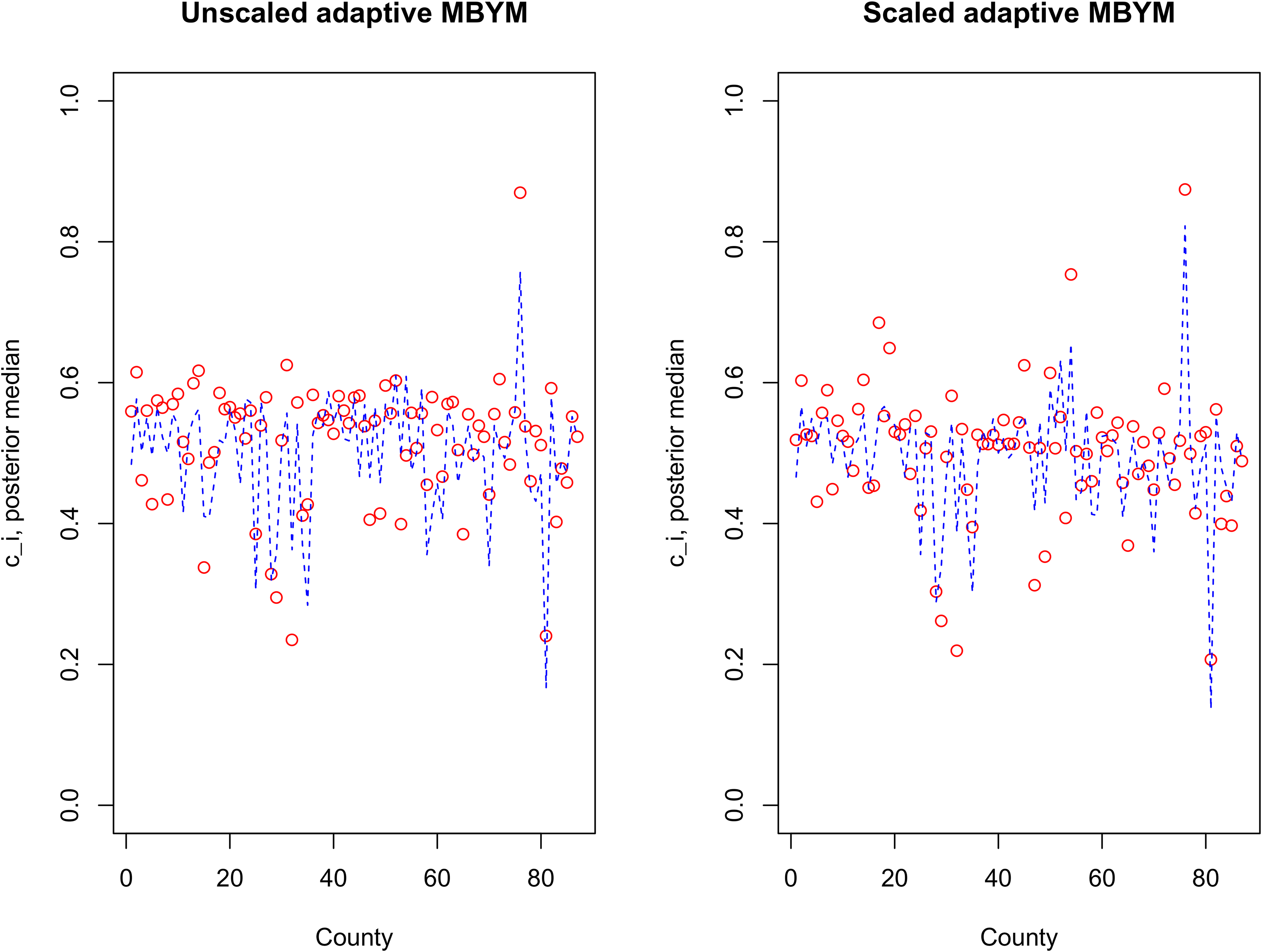
Posterior median of
Posterior estimates, median and standard deviation (sd), of adaptive spatial weight parameters for three illustrative counties, GLMM (adaptive MBYM) without covariate (0 covar.) or with five covariates (5 covar.).
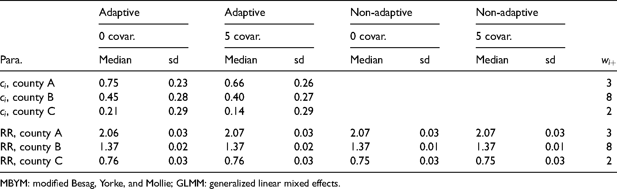
MBYM: modified Besag, Yorke, and Mollie; GLMM: generalized linear mixed effects.
This study adds to the Bayesian disease mapping literature in several respects. Analytically and via graphical visualization, we showed that these risk models are Gaussian (Markov) random fields with different spatial dependence (influence) and correlation (covariance) functions. Consequently, they and their multivariate and adaptive model extensions can play different roles in disease mapping applications of contemporary scope and complexity.
Our simulation and case studies, for their scope in illustrating and assessing the iCAR, pCAR, LCAR and (M)BYM risk models together using simulated and real data of extremely small, small, modest and large sample sizes, provided a wealth of important information on the Bayesian posterior estimation, learning, and inference of the model parameters and associated risk prediction and inference, and on the use of DIC and WAIC as tools for evaluations of estimation and out-of-sample predictive models.
In addition, a new proposal of adaptive MBYM is presented and illustrated; it illustrates how the existing spatial risk models can be broadened and extended. We discussed and illustrated the various roles the iCAR, pCAR, LCAR and (M)BYM may play in Bayesian disease mapping, for which we summarize here as takeaway messages.
The pCAR and LCAR are full rank GMRFs that can play nuanced roles of modelling spatial dependence and local influence functions regulated by their respective spatial parameters. The analytic and simulation results favoured LCAR over pCAR when mapping risks of weak or strong spatial correlations. However, pCAR as a spatial model has the advantage for its rich options of multivariate and adaptive generalizations with flexible (multidimensional) spatial dependence and local influence functions.18,23 For risk prediction and inference in the context of mapping spatially correlated disease risks, our analytic, simulation and case studies led to consistent results that the two CARs can approximate each other quite well.
The iCAR is a singular GMRF and has an unappealing covariance matrix assuming negative correlations between ‘distance areas’, which may be one reason that it was not favoured as an out-of-sample predictive model in the simulation study. Nevertheless, as an ‘a priori’ spatial smoother, it can be used as a spatial risk prior for modelling spatially structured risk heterogeneity in hierarchical Bayesian models. For the purpose of borrowing information for disease risk mapping, our simulation and case studies suggested that it can be the statistically efficient spatial risk smoother among the five when spatially correlated risks of rare diseases are under study.
The (M)BYMs have dense precision and covariance matrices that postulate practically unappealing but low negative risks dependencies and correlations between ‘distance’ areas. However, they are full rank Gaussian random fields with spatially clustered correlation and partial correlation functions postulating positive risks dependencies and correlations between neighbouring areas. While the utility of (M)BYM for modelling spatial risk dependencies remains a topic of future research, our study suggested evidence that they can be used as (1) estimation and prediction models and (2) as random effects priors for modelling additive components of spatially and randomly varying effects. Compared to fitting the MBYM(
Via simulation and case studies, we illustrated that, gaining identifiability via weakly informative prior Uniform(0, a) for the BYM scale parameters or via re-parameterization for MBYM, the BYM and MBYM can facilitate characterization of risk effects
The new adaptive MBYM is proposed and illustrated for more flexible posterior risk estimation and inference and for unveiling neighbourhood risks clusters and heterogeneities. In a recent study, MacNab 18 showed, analytically and via a case study, that adaptive extensions of the iCAR, pCAR and LCAR lead to CAR models of different local influence functions; they can be used to model different patterns of locally varying influence functions that characterize local dependencies and spatial discontinuities.
Consistent with the analytic results presented herein and in MacNab,6,27 our simulation and case studies also suggested that among the commonly used risk priors none was shown to significantly outperform the others in all disease mapping applications. Noted in MacNab,6,18 and suggested by the results of the current study, Bayesian sensitivity analysis with respect to posterior risks prediction and inference, with goodness-of-fit, predictive accuracy, and model complexity assessments such as the DIC and WAIC scores being evaluated and illustrated herein (or model assessment criterions not discussed herein), is still a viable approach for model evaluation, comparison and selection. More importantly, the risk models discussed herein for their nuanced roles in disease mapping can be used as competing or complementary methods for in-depth analysis of disease mapping data.
For data of small or modest sample size, informative hyper-priors for pCAR or LCAR or MBYM spatial parameters can significantly reduce its posterior bias and uncertainty, as illustrated in our simulation and case studies. The present study also showed that both the BYM and MBYM enable (nearly) unbiased posterior estimation of the spatial and non-spatial components
Supplemental Material
sj-pdf-1-smm-10.1177_09622802221129040 - Supplemental material for Revisiting Gaussian Markov random fields and Bayesian disease mapping
Supplemental material, sj-pdf-1-smm-10.1177_09622802221129040 for Revisiting Gaussian Markov random fields and Bayesian disease mapping by Ying C MacNab in Statistical Methods in Medical Research
Footnotes
Acknowledgements
This research was funded in part by a discovery grant (RGPIN 238660-13) from the Natural Sciences and Engineering Research Council of Canada.
Declaration of conflicting interests
The authors declared no potential conflicts of interest with respect to the research, authorship, and/or publication of this article.
Funding
The authors received no financial support for the research, authorship, and/or publication of this article.
Supplemental material
Supplemental material for this article is available online.
References
Supplementary Material
Please find the following supplemental material available below.
For Open Access articles published under a Creative Commons License, all supplemental material carries the same license as the article it is associated with.
For non-Open Access articles published, all supplemental material carries a non-exclusive license, and permission requests for re-use of supplemental material or any part of supplemental material shall be sent directly to the copyright owner as specified in the copyright notice associated with the article.