Inference on latent factor models for informative censoring

Abstract

This work discusses the problem of informative censoring in survival studies. A joint model for the time to event and the time to censoring is presented. Their hazard functions include a latent factor in order to identify this joint model without sacrificing the flexibility of the parametric specification. Furthermore, a fully Bayesian formulation with a semi-parametric proportional hazard function is provided. Similar latent variable models have been described in literature, but here the emphasis is on the performance of the inferential task of the resulting mixture model with unknown number of components. The posterior distribution of the parameters is estimated using Hamiltonian Monte Carlo methods implemented in Stan. Simulation studies are provided to study its performance and the methodology is implemented for the analysis of the ACTG175 clinical trial dataset yielding a better fit. The results are also compared to the non-informative censoring case to show that ignoring informative censoring may lead to serious biases.

Introduction

Right-censored survival times are very common in event time studies. Right-censoring is non-informative if the censoring times do not depend on the event of interest. For instance, units whose event of interest has not occurred by the end of the clinical study (type I censoring). Conversely, units may drop out from the study for reasons which depend on the event of interest. For example, in a clinical study on the efficacy of a new treatment, a patient may withdraw due to the worsening of their medical conditions.

In case of informative censoring, we need to consider a model for the joint distribution of the censoring time $C$ and the time to event $T$ . Not addressing this dependency between $T$ and $C$ may result in a biased estimation of the distribution of $T$ . However, this joint distribution is not identifiable given the data, since we only observe the minimum between $C$ and $T$ (see ¹ , ² and ³ for a more detailed account of this issue). Thus, we have to make untestable assumptions if we wish to study the joint distribution of $T$ and $C$ .

Some examples from the literature are the works of ⁴ , who proposed and analysed the use of a bivariate Weibull model for $(T,C)$ , and the work of ⁵ who analyse the consistency of the estimator of the marginal survival function of $T$ and $C$ based on a copula model with known dependence parameters. These parametric models are typically used to investigate sensitivity with respect to the dependency parameter.

Scharfstein and Robins ⁶ consider a hazard function specification for the censoring time which has a multiplicative relationship with a function of $T$ , while ⁷ specify a semi-parametric hazard function ( ⁸ ) for $T$ , which has a step-change associated with the censoring event. In this way, they avoid modeling the marginal distribution of $C$ . The limitation of these approaches is their need to fix the parameter which calibrates the degree of dependence between $T$ and $C$ , since it cannot be estimated on the basis of available data.

Huang and Wolfe ⁹ proposed the use of a latent variable to account for the dependency between $T$ and $C$ . Given this latent variable, then $T$ and $C$ are independently distributed. They assume that this latent variable is normally distributed with mean zero and unknown variance. This latent variable operates on a cluster level (e.g., clinics with patients) where each cluster has its own frailty, which is shared by all units in the cluster. The limitation of this approach is that the parametric class of distributions for the latent variable must be known.

Rowley et al. ¹⁰ extended the work of ⁹ by considering a latent factor with a finite but unknown number of possible outcomes. The resulting joint distribution of $T$ and $C$ turns out to be a mixture distribution with an unknown number of components. The authors suggested to estimate this joint distribution with the Maximum-a-Posteriori (MAP) estimator and they recommended to determine the number of levels with the Bayesian Information Criterion (BIC).

Among all options of modeling the joint distribution of T and C, the latent variable approach seems to be the most promising, since it has the least limitations compared to alternative parametric hazard function specifications.

However, statistical models including latent factors, such as those proposed in ¹⁰ , contain singularities in their parameter space, which means that there is not a one-to-one mapping from the parameter space to a probability distribution. As a consequence, the Fisher Information Matrix may not be invertible (see ¹¹ and ¹² ). Thus, estimators like maximum likelihood (ML) and MAP do not have asymptotic normal distributions and may yield divergent parameter estimates when applied to real datasets. The asymptotic distribution of the parameter estimators deviates from being Gaussian in ill-posed models, particularly when the estimator reaches the boundary of the parameter space ( ¹³ ). When dealing with mixture distributions this problem occurs when the mixture weight is close to zero, when two mixture components are very close to one another, or more generally when a mixture in $K$ components can be equivalently obtained as a mixture in $K^{\prime }$ components, with $K^{\prime }<K$ .

The problem of model selection between distributions with different number of mixture components turns out to be extremely critical in this context. Classical information criteria such as the AIC ( ¹⁴ ) and the BIC ( ¹⁵ ) cannot be used (see ¹⁶ for further details).

Another criticism towards the use of ML and MAP estimators is that for a mixture model with $K$ components the likelihood function is most likely multimodal. Fitting a $K$ -component mixture model on $n$ observations, results in a likelihood function of the form of a sum of $K^n$ terms, each corresponding to the likelihood function obtainable under the possible realizations of the latent factor. Thus, there may exist multiple roots, and the observed solution can be affected by the choice of the starting values. Finally, the numerical optimization can require high computational time, due to the large number of parameters and the complexity of the objective function, and there would not be any guarantee that all roots will be found.

This work focuses on a joint model for $T$ and $C$ , where they are independently distributed conditional on a latent class or factor $H$ , similar as in ¹⁰ . A point-identifying assumption for this distribution is specified, without sacrificing the flexibility of the parametric model.

We propose the use of a fully Bayesian analysis, where instead of focusing on a point estimate, we try to estimate the posterior distribution of the parameters. The contribution of this work is thus to address the inferential challenges posed by these mixture models for addressing informative censoring in survival models. We will discuss identifiability, the Bayesian inference for this model, including prior specification and parametrization of the mixture model, and the model selection problem for mixture distributions with unknown number of components.

Section 2 will discuss these model formulations, while Section 3 addresses the estimation problem within the Bayesian inferential paradigm. Section 4 contains a simulation study to assess the performance of the inferential strategy described in Section 3. As an illustrative example the ACTG175 clinical trial ( ¹⁷ ) is analysed, and the results are illustrated in Section 5. Extension of the use of joint models with latent factors are discussed in Section 6. Finally, Section 7 provides a summary and a discussion.

Modeling non-informative censoring with latent factors

In our model we assume that the event time $T$ and the censoring time $C$ are conditionally independent given latent factor $H$ . Thus the joint density of $(T,C)$ is given by:

$$f(t,c)={\int }_h{f}_{T\mid H}(t\mid h)f_{C\mid H}(c\mid h)d{F}_H\left(h\right)$$

(1)

where $f(\cdot )$ denotes the density function while $F(\cdot )$ denotes the distribution function. We refer to the latent factor $H$ as the frailty.

Furthermore, we allow that the distribution of $T$ and $C$ may depend on a vector of time varying covariates at time $u\in [0,\mathrm{\infty })$ , denoted by $x^T(u)=(x_1^T(u),\dots ,x_{P_T}^T(u))$ and $x^C(u)=(x_1^C(u),\dots ,x_{P_C}^C(u))$ respectively. In this work, we include covariates by means of the Cox proportional hazard model ( ⁸ ). We assume that the distribution of $H$ is independent of $x^T(\cdot )$ and $x^C(\cdot )$ .

Model

We assume that the latent factor $H$ is a discrete variable which takes $K+1$ possible values, denoted for simplicity by the set of integers $\{0,1,\dots ,K\}$ . $K$ is considered to be fixed but unknown. We set $H=0$ as the baseline level, and write $h=(h_1,\dots ,h_K)$ , such that $h_k={\mathbb{1}}_{[H=k]}$ .

The following models for the hazard function of $T$ and $C$ are considered:

$${\mu }^T(u\mid x^T(u),h;{\beta }^T,{\gamma }^T)={\mu }_0^T\left(u\right)\exp ({\beta }^{T^{\prime }}{x}^T(u)+{\gamma }^{T^{\prime }}h)$$

(2)

$${\mu }^C(u\mid x^C(u),h;{\beta }^C,{\gamma }^C)={\mu }_0^C\left(u\right)\exp ({\beta }^{C^{\prime }}{x}^C(u)+{\gamma }^{C^{\prime }}h)$$

(3)

where ${\beta }^{\ell }$ is the vector of regression coefficients capturing the effect of the covariates $x^{\ell }(\cdot )$ , and ${\mu }_0^{\ell }(\cdot )$ is the baseline hazard function. The unknown parameters ${\gamma }^{\ell }=({\gamma }_0^{\ell },\dots ,{\gamma }_K^{\ell })$ capture the proportional effect of each outcome of $H$ on the the hazard ( $\ell \in \{T,C\}$ ). We assume that ${\gamma }_0^{\ell }=0$ .

As result, now the frailty component has a discrete distribution with sample space $(1,\exp ({\gamma }_1^{\ell }),\dots ,\exp ({\gamma }_K^{\ell }))$ , for $\ell \in \{T,C\}$ .

¹⁰ also allow for the possibility of regression parameters $\beta$ which depend on $H$ , and the distribution of $H$ may depend on $X$ . An even more structured model, would allow $H$ to be time-varying.

The latent factor $H$ can be interpreted as an underlying health state or situation of a (group of) patient(s). For example, whether a patient used zidovudine for HIV Type I infection. In this case, the number of levels $K$ for latent factor $H$ is known and equal to two.

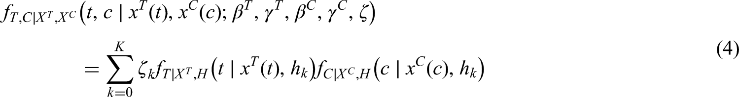
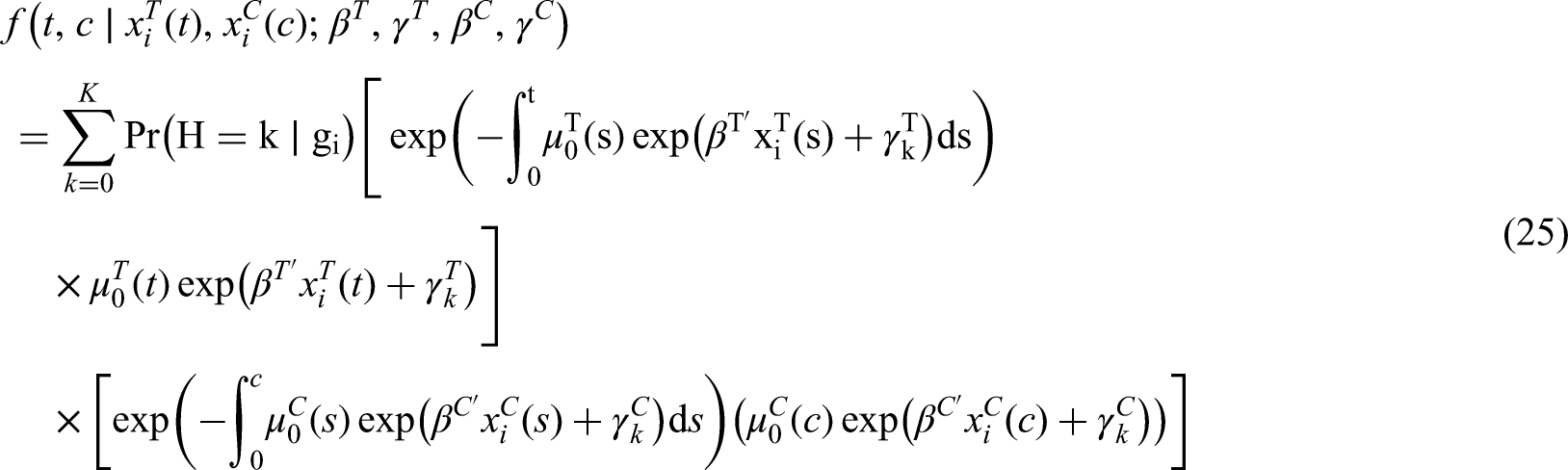
The resulting joint distribution of $T$ and $C$ still corresponds to the integral of equation (1), where the frailty component is dominated by the counting measure, hence the density can be rewritten as follows:

$$\begin{array}{rl}{f}_{T,C\mid X^T,X^C}& (t,c\mid x^T(t),x^C(c);{\beta }^T,{\gamma }^T,{\beta }^C,{\gamma }^C,\zeta )\\ & ={\displaystyle \sum _{k=0}^K{\zeta }_k{f}_{T\mid X^T,H}(t\mid x^T(t),h_k)f_{C\mid X^C,H}(c\mid x^C(c),h_k)}\end{array}$$

(4)

where $\zeta =({\zeta }_0,\dots ,{\zeta }_K)$ and ${\zeta }_k=\text{Pr}(H=k)$ . Equation (4) is in fact a mixture distribution with $K+1$ components induced by the presence of a latent factor $H$ . $\zeta$ can be considered as the non-parametric distribution of $H$ (see^{18,19, 20} ).

The mixture formulation also accounts for non-informative censoring, which occurs when either one or both conditions hold:

• i) ${\gamma }_0^T=\dots ={\gamma }_K^T=0$ ;

• ii) ${\gamma }_0^C=\dots ={\gamma }_K^C=0$ ;

In particular, in situation i) we obtain the Cox proportional hazards model without heterogeneity between patients in hazard for the time to event $T$ , while in ii) the hazard function for $T$ is still characterized by sources of heterogeneity which are not explained by the censoring mechanism.

Identifiability

General conditions for the identifiability of this modelling approach have been analysed in ²¹ , ²² and ²³ .

Nevertheless, given the finite mixture nature of our approach, two additional conditions are needed to ensure its global identifiability ¹ (see also ²⁵ and ²⁶ ):

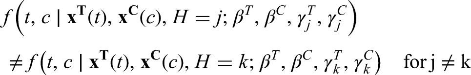
For every value of $(t,c,{\mathbf{x}}^{\mathbf{T}}(t),{\mathbf{x}}^{\mathbf{C}}(c))$ , different values of $H$ should result into different p.d.f.s:

$$\begin{array}{rll}& f(t,c\mid {\mathbf{x}}^{\mathbf{T}}\left(t\right),{\mathbf{x}}^{\mathbf{C}}\left(c\right),H=j;{\beta }^T,{\beta }^C,{\gamma }_j^T,{\gamma }_j^C)& \\ & \ne f(t,c\mid {\mathbf{x}}^{\mathbf{T}}\left(t\right),{\mathbf{x}}^{\mathbf{C}}\left(c\right),H=k;{\beta }^T,{\beta }^C,{\gamma }_k^T,{\gamma }_k^C)\text{ for }j\ne k\end{array}$$

and thus two different hazard functions for $T$ or two different hazard function for $C$ given their conditional independence;

$0<{\zeta }_k<1$ for $k=0,\dots ,K$ . This condition is needed because if for any $k$ we have ${\zeta }_k=0$ , then ${\gamma }_k^T$ and ${\gamma }_k^C$ can take any value without affecting the mixture distribution.

However, the joint probability distribution of $(T,C)$ outlined so far is not locally identifiable: by permuting the labels of $H$ , we obtain exactly the same joint p.d.f.:

$$\begin{array}{rl}& {\displaystyle \sum _{k=0}^K{\zeta }_k\left[\exp (-{\int }_0^t{\mu }^T(s\mid x^T(s),h;{\beta }^T,{\gamma }_k^T)\mathrm{d}s){\mu }^T(t\mid x^T(t),h;{\beta }^T,{\gamma }_k^T)\right]}\\ & \times \left[\exp (-{\int }_0^c{\mu }^C(s\mid x^C(s),h;{\beta }^C,{\gamma }_k^C)\mathrm{d}s){\mu }^C(c\mid x^C(c),h;{\beta }^C,{\gamma }_k^C)\right]\\ & ={\displaystyle \sum _{k=0}^K{\zeta }_{\rho \left(k\right)}\left[\exp (-{\int }_0^t{\mu }^T(s\mid x^T(s),h;{\beta }^T,{\gamma }_{\rho \left(k\right)}^T)\mathrm{d}s){\mu }^T(t\mid x^T(t),h;{\beta }^T,{\gamma }_{\rho \left(k\right)}^T)\right]}\\ & \times \left[\exp (-{\int }_0^c{\mu }^C(s\mid x^C(s),h;{\beta }^C,{\gamma }_{\rho \left(k\right)}^C)\mathrm{d}s){\mu }^C(c\mid x^C(c),h;{\beta }^C,{\gamma }_{\rho \left(k\right)}^C)\right]\end{array}$$

where $\rho (k)$ represents any permutation of the indexing given by $k$ , and $\sum _{k=0}^K{\zeta }_k=1$ .

This problem can be easily overcome by restricting the parameter space of the hazard function. In Section 3.2 we address this issue in the perspective of improving the efficiency of the Hamiltonian Monte Carlo sampler.

Inference

For the reasons described in Section 1, in this work we carry out our inferential exercise using Bayesian techniques. Let $p({\beta }^T,{\gamma }^T,{\beta }^C,{\gamma }^C,\zeta \mid K)$ denote the $K$ -dependent prior distribution of the parameter vector $({\beta }^T,{\gamma }^T,{\beta }^C,{\gamma }^C,\zeta )$ . The learning object is thus given by the following posterior distribution of the vector $({\beta }^T,{\gamma }^T,{\beta }^C,{\gamma }^C,\zeta )$ :

$$\begin{array}{rl}& p({\beta }^T,{\gamma }^T,{\beta }^C,{\gamma }^C,\zeta \mid \text{data},K)\propto p({\beta }^T,{\gamma }^T,{\beta }^C,{\gamma }^C,\zeta \mid K)L({\beta }^T,{\gamma }^T,{\beta }^C,{\gamma }^C,\zeta \mid \text{data},K)\\ & =p({\gamma }^T,{\gamma }^C,\zeta \mid K,{\beta }^T,{\beta }^C)p({\beta }^T,{\beta }^C)L({\beta }^T,{\gamma }^T,{\beta }^C,{\gamma }^C,\zeta \mid \text{data},K)\end{array}$$

(5)

where $L({\beta }^T,{\gamma }^T,{\beta }^C,{\gamma }^C,\zeta \mid \text{data},K)$ denotes the likelihood as a function of the parameters, given the data and $K$ . In order to avoid the use of a cumbersome notation $p$ will denote the density function of the parameters.

In equation (5) we remarked the dependence of the posterior distribution on $K$ , since it determines the dimension of the parameter space, particularly for ${\gamma }^T$ , ${\gamma }^C$ and $\zeta$ .

Likelihood function

Let us first distinguish $C$ from $C^{*}$ , where the former denotes the time to informative censoring, and the latter denotes the time to non-informative censoring (e.g. administrative censoring). Let $T^{\prime }=\text{min}(T,C,C^{*})$ , $d_i={\mathbb{1}}_{[t_i^{\prime }=t_i]}$ and $d_i^{*}={\mathbb{1}}_{[t_i^{\prime }=c_i]}$ . Thus, if a time to event is subject to non-informative censoring, then $d_i=d_i^{*}=0$ .

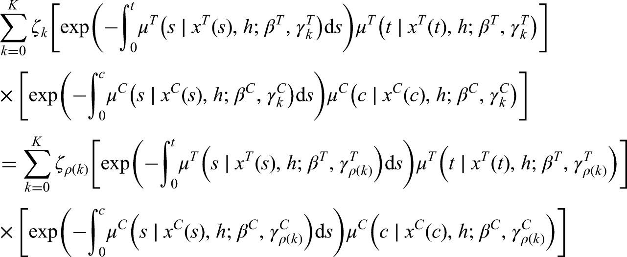
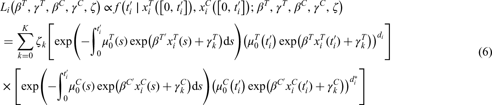
The latent factor $H$ is never observed, hence the $i$ th individual likelihood contribution must be marginalized with respect to $H$ :

$$\begin{array}{rl}& L_i({\beta }^T,{\gamma }^T,{\beta }^C,{\gamma }^C,\zeta )\propto f(t_i^{\prime }\mid x_i^T\left([0,t_i^{\prime }]\right),x_i^C\left([0,t_i^{\prime }]\right);{\beta }^T,{\gamma }^T,{\beta }^C,{\gamma }^C,\zeta )\\ & ={\displaystyle \sum _{k=0}^K{\zeta }_k\left[\exp (-{\int }_0^{t_i^{\prime }}{\mu }_0^T\left(s\right)\exp ({\beta }^{T^{\prime }}{x}_i^T(s)+{\gamma }_k^T)\mathrm{d}s){\left({\mu }_0^T\left(t_i^{\prime }\right)\exp ({\beta }^T{x}_i^T(t_i^{\prime })+{\gamma }_k^T)\right)}^{d_i}\right]}\\ & \times \left[\exp (-{\int }_0^{t_i^{\prime }}{\mu }_0^C\left(s\right)\exp ({\beta }^{C^{\prime }}{x}_i^C(s)+{\gamma }_k^C)\mathrm{d}s){\left({\mu }_0^C\left(t_i^{\prime }\right)\exp ({\beta }^{C^{\prime }}{x}_i^C(t_i^{\prime })+{\gamma }_k^C)\right)}^{d_i^{*}}\right]\end{array}$$

(6)

where ${\gamma }_0^{\ell }=0$ and $x_i^{\ell }(s)$ for $\ell \in \{T,C\}$ is the set of covariates value at time $s\in [0,t_i^{\prime }]$ .

In equation (6) the covariates are assumed as continuously observed throughout the whole time span $[0,t_i^{\prime }]$ . In practice, covariates are observed at discrete time points, and several assumptions can be made for their value at intermediate time points. For example, in the simulation study (Section 4) and in the empirical analysis (Section 5) the covariates are assumed constant between two observation times, and equal to the previously observed value.

The resulting likelihood function of the parameters, given the data $L({\beta }^T,{\gamma }^T,{\beta }^C,{\gamma }^C,\zeta \mid \text{data})=\prod _i{L}_i({\beta }^T,{\gamma }^T,{\beta }^C,{\gamma }^C,\zeta )$ is the sum of $(K+1{)}^n$ terms, each corresponding to a realization of the latent factor for each unit in the sample.

Prior specification and model reparametrization

In general, the Bayesian analysis of a mixture model is particularly challenging. For this reason, the prior should be chosen accurately, and the model needs to be parametrized in a way that makes the sampling process efficient.

First of all, we assume for convenience that the vectors ${\beta }^T$ , ${\beta }^C$ , ${\gamma }^T$ , ${\gamma }^C$ and $\zeta$ are pairwise independently distributed, that is:

$$p({\beta }^T,{\gamma }^T,{\beta }^C,{\gamma }^C,\zeta \mid K)=p\left({\beta }^T\right)p\left({\beta }^C\right)p({\gamma }^T\mid K)p({\gamma }^C\mid K)p(\zeta \mid K)$$

(7)

where each density depends on some hyperparameters.

The specification of the prior distribution for the regression coefficient parameters ${\beta }^T$ and ${\beta }^C$ does not represent a problem, hence it is possible to specify a non-informative prior in order to reduce the extent of subjective assumptions on the inference.

The prior distribution of ${\gamma }^T$ , ${\gamma }^C$ and $\zeta$ must be specified with more care. The use of prior distributions which are at least weakly informative is appropriate, in order to enhance the efficiency of the sampler.

For example, with the use of an exchangeable prior on $({\gamma }_1^T,\dots ,{\gamma }_K^T)$ , $({\gamma }_1^C,\dots ,{\gamma }_K^C)$ and of a uniform prior on $\zeta$ ² , then their posterior distribution will maintain the permutation invariance induced by the mixture likelihood ( ²⁷ and ²⁸ ).

This multimodality hinders the efficiency of the sampler, because it would take a large number of iterations to fully explore the posterior distribution. Indeed, the sampler is likely to get stuck in an area of the parameter space corresponding to one mode of the posterior distribution (see ²⁹ ).

In Bayesian inference the identifiability of a mixture distribution turns out to be more crucial. In Section 2.2 we mentioned how a constraint allows for a model to be identifiable. In our case we also need to follow a strategy which allows for an efficient sampling for the posterior distribution.

For the joint distribution of equation (4), we need to place an ordering constraint on the set $[({\gamma }_1^T,{\gamma }_1^C),\dots ,({\gamma }_K^T,{\gamma }_K^C)]$ , which can be done by ordering either $({\gamma }_1^T,\dots ,{\gamma }_K^T)$ or $({\gamma }_1^C,\dots ,{\gamma }_K^C)$ . For example, we can set:

$$0<{\gamma }_1^T<{\gamma }_2^T<\dots <{\gamma }_K^T$$

(8)

where we take into account also the component corresponding to ${\gamma }_0^T=0$ . An account of the geometric interpretation of this constraint can be found in ²⁸ . This constraint also turns exchangeable priors into nonexchangeable ones due to the restriction of the parameter space into its subset, singling out one mode of the posterior distribution, as induced by the label permutation. Conversely, the exchangeability in the prior distribution will be inherited also by the posterior distribution.

However, when the mixture components are not well separated (i.e. these are very close to one another in value), then also the posterior distribution will be affected by the imposed constraint. For example, suppose we set an ordering as in equation (8), and there is a nonnegative probability that ${\gamma }_1^T>{\gamma }_2^T$ (all else being equal, which is more likely if ${\gamma }_1^T$ is very close to ${\gamma }_2^T$ ), then the true posterior distribution cannot be captured by the posterior distribution satisfying such constraint.

In the extreme case where the mixture components overlap, then the posterior distribution will be more difficult to explore ( ²⁸ ), as may occur when the value of $K$ is larger than actually needed to explain the heterogeneity among the units. In this case the components in excess will collapse into those which are necessary and have been already included in the model.

This justifies our inferential strategy of analyzing increasingly complex models in terms of needed mixture components, as we describe in Section 3.3.

Choice of the number of mixture components

The value of $K$ is inferred by solving a model selection problem, where models with different values of $K$ are separately fitted and then compared to one another using appropriate information criteria. Algebraic geometry tools have been proven useful in order to understand the asymptotic behavior of the posterior distribution of the parameters when dealing with singular statistical models. For example, ¹¹ proposes the Widely Applicable Information Criterion (WAIC), which generalizes the AIC to the analysis of singular models.

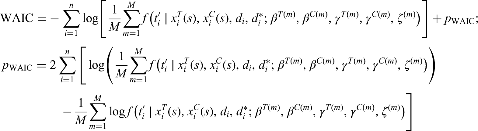
The WAIC is computed as follows (notation simplified for ease of exposition):

$$\begin{array}{rl}\text{WAIC}=& -{\displaystyle \sum _{i=1}^n\log \left[\frac{1}{M}{\displaystyle \sum _{m=1}^{M}f(t_i^{\prime }\mid x_i^T\left(s\right),x_i^C\left(s\right),d_i,d_i^{*};{\beta }^{T(m)},{\beta }^{C(m)},{\gamma }^{T(m)},{\gamma }^{C(m)},{\zeta }^{(m)})}\right]+p_{\text{WAIC}};}\\ & p_{\text{WAIC}}=2{\displaystyle \sum _{i=1}^n[\log \left(\frac{1}{M}{\displaystyle \sum _{m=1}^{M}f(t_i^{\prime }\mid x_i^T\left(s\right),x_i^C\left(s\right),d_i,d_i^{*};{\beta }^{T(m)},{\beta }^{C(m)},{\gamma }^{T(m)},{\gamma }^{C(m)},{\zeta }^{(m)})}\right)}\\ & -\frac{1}{M}{\displaystyle \sum _{m=1}^M\log f(t_i^{\prime }\mid x_i^T\left(s\right),x_i^C\left(s\right),d_i,d_i^{*};{\beta }^{T(m)},{\beta }^{C(m)},{\gamma }^{T(m)},{\gamma }^{C(m)},{\zeta }^{(m)})]}\end{array}$$

where $M$ is the number of sampled values from the posterior distribution of the parameters, and $p_{\text{WAIC}}$ is a penalization term which can be interpreted as the effective number of parameters, and measures the fluctuation of the posterior distribution (see ¹⁶ ).

Our strategy is to first analyze the model with $K=0$ ( $T$ and $C$ independently distributed given $x^T(\cdot )$ and $x^C(\cdot )$ ) and then we fit models with increasing $K$ until the WAIC does not decrease, as we aim at its minimization.

Similar information criterion have been proposed to generalize the BIC, such as the singular BIC of ¹² and the Widely Applicable Bayesian Information Criterion (WBIC) of ³⁰ . The former is of harder implementation in practice, while we found in a simulation study (not discussed here) that the WBIC shows a slightly better performance than the WAIC in selecting the true model, particularly when the mixture components are well separated. The WAIC is hereby preferred over the BIC generalization for two practical reasons: i) it provides a measure of model dimension through $p_{\text{WAIC}}$ ; ii) it turns out to be more practical since it allows to use the same output from the posterior sampling process.

Estimation

For the estimation of the posterior distribution of equation (5) we use the Hamiltonian Monte Carlo (HMC) sampler (see ³¹ ). This algorithm belongs to the general Metropolis-Hastings family. HMC uses Hamiltonian dynamics which allow for a faster exploration of the parameter space. It turns out to be more efficient than more traditional Gibbs and random-walk Metropolis samplers for posterior distributions showing high correlations among the parameters, as it occurs for mixture distributions.

The HMC sampler is implemented by using the Stan software package ( ³² ) and its R interface ( ³³ ), by means of the package rstan. In its default implementation Stan uses the No-U-Turn sampler of ³⁴ which allows for an automatic tuning of the sampler. Furthermore, the rstan can automatically initialize the sampling process.

Simulation study

Set up

Simulation studies are carried out to assess the performance of the methodology outlined in this work. We focus on the posterior distribution of the parameters ${\beta }^T$ , ${\beta }^C$ , ${\gamma }^T$ and ${\gamma }^C$ , and thus on whether the WAIC allows to chose the true model. We look at whether the 95% credible intervals of the posterior distribution include the true value of the parameters, and we analyse whether the posterior mean can be considered as an unbiased point estimate of the parameters.

We compare these results with the parameter estimates and the 95% coverage intervals obtainable from the Cox proportional hazards model. This gives us the opportunity to quantify the need for our method in certain settings.

For each simulation run, we generate samples of 500 potentially censored lifetimes.

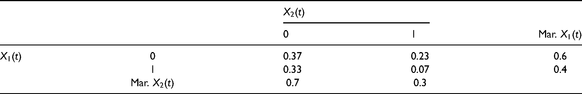
For each patient we assume the vector of time-varying binary covariates $X(t)=X^T(t)=X^C(t)=(X_1(t),X_2(t))$ (for example treatment and disease) with the probability distribution shown in Table 1.

Table 1.

Joint probability distribution of $(X_1(t),X_2(t))$ .

		$X_2(t)$
		0	1	Mar. $X_1(t)$
$X_1(t)$	0	0.37	0.23	0.6
	1	0.33	0.07	0.4
	Mar. $X_2(t)$	0.7	0.3

The binary covariate variables $(X_1(t),X_2(t))$ are independent throughout time.

We consider an observational period of 8 years, and a follow up period of 4 years for simplicity such that the researcher observes $X(t)$ for $t=0,4,8$ . In medical practice, these values can change at very high frequency over time, for example whether a patient has a high or low blood pressure, or the time-dependent treatment, although applied statistical analyses contain simplifications to overcome the issue. In this simulation study we assume that $X(t)$ is constant between one observation and the other.

For each unit, $H$ is generated from a $\text{Mult}(1,\zeta )$ distribution.

For $K=1$ we consider two scenarios: the case of well separated mixture components (WS), and the case of poorly separated mixture components (PS).

In the WS scenario $T$ and $C$ are generated under the following hazard functions:

$${\mu }^T(u\mid x^T(u),h;{\beta }^T,{\gamma }^T)=\exp (-1.2-0.9x_1(u)+0.8x_2(u)+2h_1)$$

(9)

$${\mu }^C(u\mid x^C(u),h;{\beta }^C,{\gamma }^C)=\exp (-2-x_1(u)+0.5x_2(u)+3.5h_1)$$

(10)

Conversely, in case of poorly separated mixture components, we specify:

$${\mu }^T(u\mid x^T(u),h;{\beta }^T,{\gamma }^T)=\exp (-0.2-0.9x_1(u)+0.8x_2(u)+0.5h_1)$$

(11)

$${\mu }^C(u\mid x^C(u),h;{\beta }^C,{\gamma }^C)=\exp (-0.5-x_1(u)+0.5x_2(u)+h_1)$$

(12)

For the case of two mixture components we set $\zeta =(0.65,0.35)$ and ${\gamma }^C$ is chosen in order to keep a stochastic ordering in the hazard function of the censoring time due to higher values of $H$ .

When $K=2$ , then $T$ and $C$ are generated according to the following hazard functions:

$${\mu }^T(u\mid x^T(u),h;{\beta }^T,{\gamma }^T)=\exp (-1+0.3x_1(u)-x_2(u)+3h_1+2h_2)$$

(13)

$${\mu }^C(u\mid x^C(u),h;{\beta }^C,{\gamma }^C)=\exp (-1.6-0.7x_1(u)+0.5x_2(u)+2.5h_1+4h_2)$$

(14)

and $\zeta =(0.48,0.32,0.2)$ . In this case, we consider only the case of well separated mixture components due to the smaller sample size.

The analysis of models with more than three mixture components requires ideally larger samples than those analysed in this work, while the case $K=0$ can be more efficiently fitted with a Cox proportional hazard model. For each value of $K$ we generate 100 datasets. In all cases we ensure that the datasets have around 40% censored units and a negligible percentage of type I censoring cases.

Drawing a value for (T,U)

A general property of survival models is that the integrated hazard function ${\int }_0^t\mu (s)\mathrm{d}s$ is a random variable with $\text{Exponential}(1)$ distribution.

Therefore, conditional on a standard uniform random variable $Z\sim \text{Unif}(0,1)$ , a set of covariates $X(t)$ and a factor $H$ , a sampled value of $T$ , denoted by $t$ , is given by the solution of the following equation:

$$-\log z={\int }_0^t{\mu }^T(s\mid x\left(s\right),h;{\beta }^T,{\gamma }^T)\mathrm{d}s$$

(15)

Given the set-up described in Section 4.1 and the hazard function specification of equations (9)-(14), then equation (15) has a closed form solution. In the same way we can sample a value for the censoring time $C$ .

Then, once $t$ and $c$ are obtained, a value for the triplet $(t^{\prime },d,d^{*})$ is calculated as follows:

$$t^{\prime }=\text{min}(t,c)$$

(16)

$$d={\mathbb{1}}_{[t\le c\le 8]}$$

(17)

$$d^{*}={\mathbb{1}}_{[c<t\le 8]}$$

(18)

Implementation

We use weakly informative prior distributions for each parameter, instead of fully non-informative ones in order to foster the convergence of the sampler. In this way, the posterior distribution will not be strongly affected by prior assumptions. Indeed, with enough observations, the effect of the prior should be negligible ( ¹⁶ ).

Furthermore, we assume that parameters are a priori independently distributed.

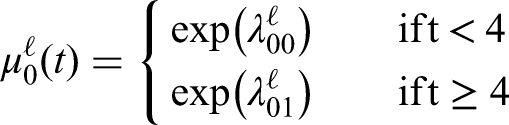
We model the baseline hazard function of $T$ and $C$ using a piecewise constant hazard function as follows:

$${\mu }_0^{\ell }(t)=\{\begin{array}{cc}\exp \left({\lambda }_{00}^{\ell }\right)& \text{if }t<4\\ \exp \left({\lambda }_{01}^{\ell }\right)& \text{if }t\ge 4\end{array}$$

where $\ell \in \{T,C\}$ , in order to ease the representation, considering a time span divided into two sub-periods of 4 years.

The posterior modeling involves ${\lambda }_0^{\ell }=({\lambda }_{00}^{\ell },{\lambda }_{01}^{\ell })$ , since in this way we do not need to constrain the parameter space, and the sampler works more efficiently.

The piecewise constant baseline hazard function represents a useful yet flexible specification, mainly if the number of knots (or intervals) increases. Alternative models can be given for example by a Gamma Process for the integrated baseline hazard function (see ³⁵ ), or the use of splines ( ³⁶ ). Further alternatives are discussed in the book of ³⁷ .

For the prior distribution we assume that ${\lambda }_0^T$ , ${\lambda }_0^C$ , ${\beta }^T$ and ${\beta }^C$ are vectors of pairwise independent and normally distributed variables with mean 0 and variance equal to 10. When fitting a model with $K=1$ we assume that ${\gamma }_1^T\sim N(0.5,100)$ , ${\gamma }_1^C\sim N(1,100)$ truncated at the lower bound of 0 and $\zeta \sim \text{Dirichlet}(30,20)$ . When $K=2$ , the prior of ${\gamma }_1^T$ and ${\gamma }_1^C$ are as before, while ${\gamma }_2^T\sim N(1,100)$ , ${\gamma }_2^C\sim N(2,100)$ truncated at the lower bound of ${\gamma }_1^C$ and $\zeta \sim \text{Dirichlet}(21,17,12)$ . In a similar fashion, when fitting a model with $K=3$ we assume ${\gamma }_3^T\sim N(2,100)$ , ${\gamma }_3^C\sim N(3,100)$ truncated at the lower bound of ${\gamma }_2^C$ and $\zeta \sim \text{Dirichlet}(20,15,10,5)$ . In all cases, when choosing the Dirichlet distribution parameters, we kept a prior sample size (the sum of the Dirichlet distribution parameters) of 50.

The HMC sampler is run for 5,000 iterations and the first half draws are discarded in order to allow for burn-in and fine-tune the No-U-Turn sampler. Indeed, given our simulation settings, 5,000 iterations are sufficient to allow for the chains to mix and obtain a stationary posterior distribution, which ensures convergence of the sampler.

Results

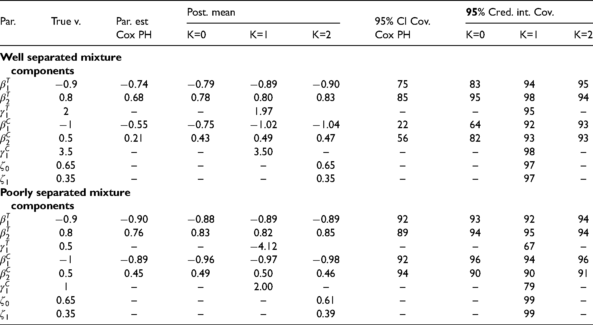
The results in Table 2 for $K=1$ show that the 95% credible intervals from the posterior distribution of the parameters include their true value with a coverage close to normal when fitting the true model $K=1$ and the mixture components are well separated. In case of lesser separated mixture components, the 95% credible intervals still show a coverage larger than 90% for ${\beta }^T$ , ${\beta }^C$ and $\zeta$ . However, the coverage sensibly decreases for ${\gamma }^T$ and ${\gamma }^C$ , whose posterior mean turns out to be divergent from their true values.

Table 2.

Parameter estimates with the Cox proportional hazard model (Cox PH), posterior mean estimate for the models with $K=0,1,2$ , coverage of the 95% confidence interval (for the Cox model) and coverage of the 95% credible intervals.

Par.	True v.	Par. est	Post. mean			95% CI Cov.	$\mathbf{95}\mathbf{\text{\%}}$ Cred. int. Cov.
		Cox PH	K=0	K=1	K=2	Cox PH	K=0	K=1	K=2
Well separated mixture components
${\beta }_1^T$	$-0.9$	$-0.74$	$-$ 0.79	$-$ 0.89	$-$ 0.90	75	83	94	95
${\beta }_2^T$	0.8	$0.68$	0.78	0.80	0.83	85	95	98	94
${\gamma }_1^T$	$2$	–	–	1.97		–	–	95	–
${\beta }_1^C$	$-1$	$-0.55$	$-$ 0.75	$-$ 1.02	$-$ 1.04	22	64	92	93
${\beta }_2^C$	$0.5$	$0.21$	0.43	0.49	0.47	56	82	93	93
${\gamma }_1^C$	$3.5$	–	–	3.50	–	–	–	98	–
${\zeta }_0$	$0.65$	–	–	–	0.65	–	–	97	–
${\zeta }_1$	$0.35$	–	–	–	0.35	–	–	97	–
Poorly separated mixture components
${\beta }_1^T$	$-0.9$	$-0.90$	$-$ 0.88	$-$ 0.89	$-$ 0.89	92	93	92	94
${\beta }_2^T$	0.8	$0.76$	0.83	0.82	0.85	89	94	95	94
${\gamma }_1^T$	0.5	–	–	$-$ 4.12		–	–	67	–
${\beta }_1^C$	$-1$	$-0.89$	$-$ 0.96	$-$ 0.97	$-$ 0.98	92	96	94	96
${\beta }_2^C$	$0.5$	$0.45$	0.49	0.50	0.46	94	90	90	91
${\gamma }_1^C$	1	–	–	2.00	–	–	–	79	–
${\zeta }_0$	$0.65$	–	–	–	0.61	–	–	99	–
${\zeta }_1$	$0.35$	–	–	–	0.39	–	–	99	–

When the mixture components are well separated, the 95% credible intervals have a coverage below nominal for almost all parameters when fitting the model assuming that $T$ and $C$ are independently distributed (K=0): ${\beta }_1^T$ and ${\beta }_2^T$ have a coverage of 83% and 95% respectively, and ${\beta }_1^C$ and ${\beta }_2^C$ are included in the credible intervals with 64% and 82% probability respectively. As expected, in case of poorly separated mixture components, without a very large sample size, the model with $K=0$ tends to show a coverage close to nominal for the parameters ${\beta }^T$ and ${\beta }^C$ . Indeed, the true model tends to be closer to the model with $K=0$ .

The results for the posterior mean follow from those of the credible intervals. We see that the regression parameters ${\beta }^T$ and ${\beta }^C$ are in line with respect to their true value when $K=1,2$ and the mixture components are well separated. Same applies for the baseline hazard (not shown) when fitting the true model with $K=1$ , as well as for ${\gamma }^T$ , ${\gamma }^C$ and $\zeta$ .

Analogous results are obtained for the model with $K=2$ as shown in Table A1 in Appendix A.1. For this particular case, with a sample of 500 units we note that the posterior mean of ${\gamma }_2^T$ is different compared to its true value, despite the credible intervals show a coverage of 92%. A closer inspection of this result showed that this is the consequence of the small number of events for those units with $H=2$ (around 5% of the observations), which causes ${\gamma }_2^T$ to be estimated with larger uncertainty.

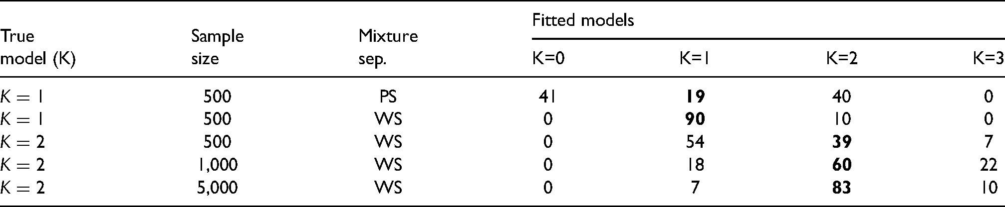
Table 3 shows that when the mixture components are well separated in all cases the WAIC excludes the lack of heterogeneity, ruling out the model with $K=0$ . In 90 cases out of 100 it selects the model with K=1, while in 10 cases it selects the model with $K=2$ . In this latter case, the WAIC for the model $K=2$ is never higher than 2 compared to the model with $K=1$ . This means that if we chose the more parsimonious model with $K=1$ , we do not lose much information. Clearly, these results depend on the values of ${\gamma }^T$ and ${\gamma }^C$ , which we purposely chose in order to ensure that the mixture components are well separated. Conversely, when the mixture components are poorly separated, in case of smaller sample sizes the models with $K=0,1,2$ tend to behave similarly. Indeed, when the WAIC picks the model with $K=0$ , then it is never larger than 1, compared to the true model with $K=1$ . Similarly, when the WAIC picks the model with $K=2$ , the difference with the WAIC for the true model is never larger than 3.2.

Table 3.

Number of times out of 100 the WAIC selects the true model based on $K$ .

True	Sample	Mixture	Fitted models
model (K)	size	sep.	K=0	K=1	K=2	K=3
$K=1$	500	PS	41	$\mathbf{19}$	40	0
$K=1$	500	WS	0	$\mathbf{90}$	10	0
$K=2$	500	WS	0	54	$\mathbf{39}$	7
$K=2$	1,000	WS	0	18	$\mathbf{60}$	22
$K=2$	5,000	WS	0	7	$\mathbf{83}$	10

Given our choice of the parameters in equations (13)–(14) related to the case $K=2$ we could see that the WAIC chooses the true model in 39 cases, while in 54 cases it chose the model with $K=1$ and in 7 cases the model with $K=3$ . The model with $K=0$ is always ruled out. When the model with $K=3$ is chosen the difference in WAIC is never higher than 1.79, and thus we reach the same conclusions as the previous cases.

These results do not necessarily mean that our approach to model selection has a poor performance as the true $K$ increases: the more complex the model, the larger the sample size should be in order to capture the heterogeneity in the units. Indeed when using a sample size of 1,000 and of 5,000 units, then the true model is selected in 60 and 83 cases out of 100 respectively. In addition, as aforementioned, also the true values of the parameter ${\gamma }^T$ and ${\gamma }^C$ play a fundamental role to capture heterogeneity among the units.

This simulation study showed how the model is always capable to spot the heterogeneity in the distribution of $T$ induced by informative censoring. Another key point is that failing to account for this heterogeneity yields a bias in the estimation of the regression coefficients, as shown by their smaller coverage. The probability of selecting the true model increases with sample size, as we can expect in highly parametrized models as analysed in this work. Parsimony is also preserved, since even when fitting a larger model which shows a better performance in terms of WAIC, then selecting a smaller model does not result in a great loss of information. Compared to the use of the Cox proportional hazard model, the results of this work are even more robust if we consider that in our model we needed to specify a baseline hazard function.

Analysis of ACTG 175 dataset

The AIDS Clinical Trial Group (ACTG) 175 study ( ¹⁷ ) is a double-blind randomised clinical trial where a total of 2,467 adults infected with HIV type I and CD4 cell counts between 200 and 500/mm ${}^3$ are randomly assigned to four different treatments: i) zidovudine, ii) didandosine, iii) zidovudine plus didandosine and iv) zidovudine plus zalcitabine.

Enrolment run from December 1991 until October 1992, while patients were scheduled to stay under analysis until November 1994. In particular, they are examined at weeks 2, 4, 8 and every 12 weeks afterwards.

For each patient we could observe baseline covariates, such as age, gender, ethnicity, CD4 count, Karnofsky score, prior use of antiretroviral therapy, haemophilia and whether the HIV was symptomatic or not; as well as some other information like the primary endpoint, and the reason for drop out from the study ³ . CD4 cell counts are checked at the initial visit and then from week 8 onwards.

The primary endpoints (the time to the event of interest we want to model in this work) of the study were a 50% decrease in CD4 cell counts with respect to the baseline, AIDS or death. At the end date of the observational study there are some patients whose primary end point did not occur, hence these can be considered as non-informatively type 1 censored.

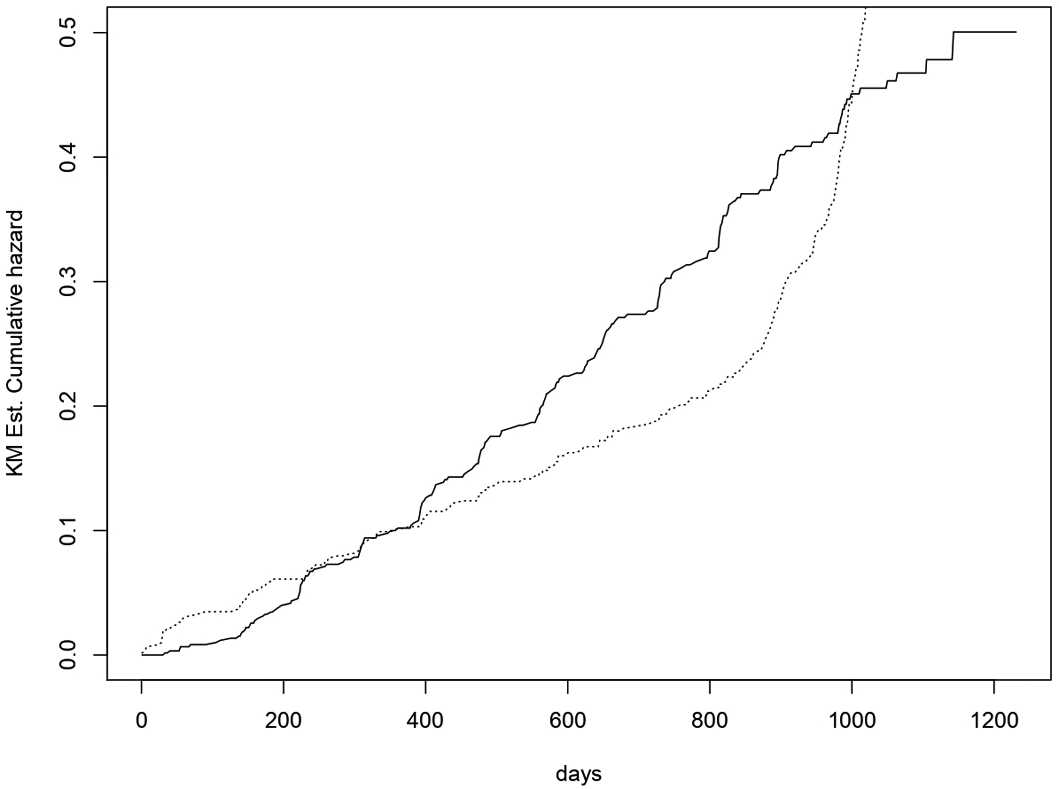
However, some other patients can drop out from the study earlier than the end date without reaching the primary endpoint for some reasons, such as toxicity of the therapy, request of the patients themselves or of the investigator, while some others just do not show up at the next planned visit (loss to follow up). In these cases it is reasonable to assume that these drop out causes are related to the primary endpoint, since for example a patient may ask to discontinue a therapy because she feels better, therefore the death event is less likely to occur (other things being equal). In this case, the Kaplan-Meier estimate of the survival function (which considers censoring as non informative) is likely to be pessimistic about patient survival.

Similar to the work of ⁶ and ³⁹ we focus on the analysis of those patients treated with zidovudine only. We thus have 614 patients of which 195 experienced the primary endpoint (151 had 50% CD4 reduction, 14 died and 30 developed AIDS).

Hence, of the remaining 419 patients, 183 are Type I censored and 236 are considered as subject to informative censoring.

Furthermore, ¹⁷ observed that throughout the study ”younger patients, those reporting injection-drug use and those with lower CD4 cell counts, lower Karnofsky score and symptoms of HIV infection at enrollment are more likely to discontinue the treatment before the study ends”.

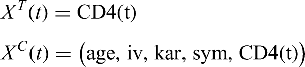
For illustration we consider the following covariates vector for $T$ and $C$ :

$$\begin{array}{rl}& X^T\left(t\right)=\text{CD4}\left(t\right)\\ & X^C\left(t\right)=(\text{age},\text{iv},\text{kar},\text{sym},\text{CD4}\left(t\right))\end{array}$$

We chose $X^T(t)$ based on the WAIC, while $X^C(t)$ is chosen on the basis of the aforementioned considerations of ¹⁷ . $X^C(t)$ is the same vector of covariates chosen in ⁶ and ³⁹ .

In particular, age denotes the age of the patient at time of randomization, iv is an indicator of intravenous drug use, kar indicates the Karnofsky score, sym is a binary variable indicating the presence of symptoms of HIV infection and CD4 $(t)$ indicates the CD4 cells count at each visit $(t)$ . We assume for simplicity that the CD4 cell count is constant between one visit and the other.

From a look at the Kaplan-Meier curve of the integrated hazard function, shown in Figure 1 we could have a rough idea about the shape of the baseline hazard function which seems approximately piecewise linear for both $T$ and $C$ . For this reason we specify a piecewise constant baseline hazard function for ${\mu }_T(\cdot )$ and ${\mu }_C(\cdot )$ with two breakpoints. As stated in Section 4.3 other specifications for the non-parametric baseline hazard function can be possible. For this dataset we noted that the use of a Gamma process would rather slower the HMC sampler without returning better results.

Figure 1.

Kaplan Meier estimate of the cumulative hazard function for T (solid line) and for the censoring (dotted line).

The breakpoints have been chosen by fitting a piecewise linear function with two breakpoints where the cumulative hazard function obtained from the Kaplan-Meier estimator is regressed against the time to event using the package segmented ( ⁴⁰ ). The breakpoint vector for ${\mu }_0^T$ is $(368.5,1006.2)$ , while the vector for ${\mu }_0^C$ is $(841,958.2)$ .

In a similar fashion with respect to the simulation study we chose weakly informative prior distributions. Hence, we assume that ${\lambda }_0^T$ , ${\lambda }_0^U$ , ${\beta }^T$ and ${\beta }^C$ are vectors of independent and normal random variables with mean 0 and standatd deviation equal to 10. ${\gamma }^T$ and ${\gamma }^C$ are chosen in the same way as in the simulation study, while assuming a prior sample size for $\zeta$ equal to 25 for all fitted models. For $K=1,2,3$ different prior distribution have been specified for $\zeta$ . This does not exclude the possibility for the researcher to use expert judgement when specifying the prior distribution. The choice of the best model is again based on the WAIC.

For each value of $K$ we run 4 parallel chains, each for 20,000 iterations (10,000 used as warm-up).

In addition, we compare these results with those obtainable from fitting a Cox proportional hazard model, which assumes independence between $T$ and $C$ .

Results

We observe that for the analysed models the HMC sampler converged towards the posterior distribution, as we can see for example from the traceplots of Figure A1, where we showed only the first two chains in Section A.2.1, and the $\hat{R}$ statistic of ⁴¹ for all parameters which is always equal to 1. The marginal posterior density of each parameter is nearly symmetric, except for ${\gamma }_1^C$ due to the chosen local identifiability constraint (Figure A2).

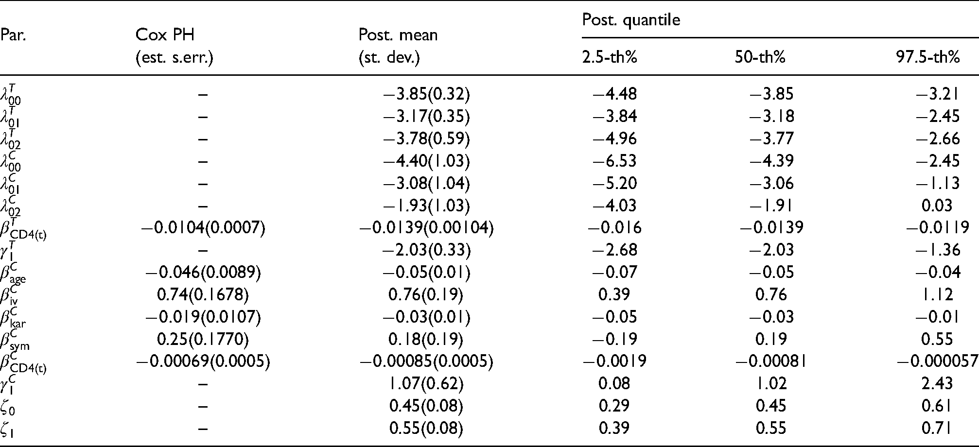
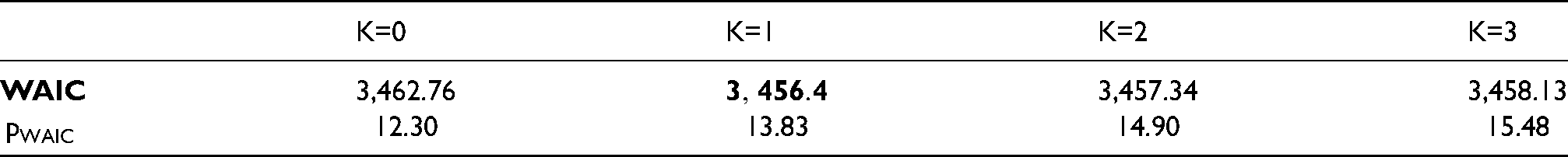
The WAIC leads to the choice of the model with $K=1$ (Table 5), whose results are shown in Table 4. As emphasized in the simulation study of Section 4 the true value of $K$ may be higher than 1 due to the relatively small sample size, although we did not have a great loss of information. As we can see, the WAIC progressively increase with $K$ after hitting its lowest point at the value of 1.

Table 4.

Cox proportional hazard model estimate of the parameters (Cox PH) and summary of the posterior distribution of the parameters for the model with $K=1$ .

Par.	Cox PH	Post. mean	Post. quantile
	(est. s.err.)	(st. dev.)	2.5-th%	50-th%	97.5-th%
${\lambda }_{00}^T$	–	$-$ 3.85(0.32)	$-$ 4.48	$-$ 3.85	$-$ 3.21
${\lambda }_{01}^T$	–	$-$ 3.17(0.35)	$-$ 3.84	$-3.18$	$-$ 2.45
${\lambda }_{02}^T$	–	$-$ 3.78(0.59)	$-$ 4.96	$-$ 3.77	$-$ 2.66
${\lambda }_{00}^C$	–	$-$ 4.40(1.03)	$-$ 6.53	$-$ 4.39	$-$ 2.45
${\lambda }_{01}^C$	–	$-$ 3.08(1.04)	$-$ 5.20	$-$ 3.06	$-$ 1.13
${\lambda }_{02}^C$	–	$-$ 1.93(1.03)	$-$ 4.03	$-$ 1.91	0.03
${\beta }_{\text{CD4( t) }}^T$	$-0.0104$ (0.0007)	$-0.0139(0.00104)$	$-0.016$	$-0.0139$	$-0.0119$
${\gamma }_1^T$	–	$-2.03(0.33)$	$-2.68$	$-2.03$	$-1.36$
${\beta }_{\text{age}}^C$	$-0.046$ (0.0089)	$-0.05$ (0.01)	$-0.07$	$-0.05$	$-0.04$
${\beta }_{\text{iv}}^C$	0.74(0.1678)	$0.76$ (0.19)	$0.39$	$0.76$	$1.12$
${\beta }_{\text{kar}}^C$	$-0.019$ (0.0107)	$-0.03$ (0.01)	$-0.05$	$-0.03$	$-0.01$
${\beta }_{\text{sym}}^C$	0.25(0.1770)	$0.18$ (0.19)	$-0.19$	$0.19$	$0.55$
${\beta }_{\text{CD4( t) }}^C$	$-0.00069$ (0.0005)	$-0.00085$ (0.0005)	$-0.0019$	$-0.00081$	$-0.000057$
${\gamma }_1^C$	–	$1.07(0.62)$	$0.08$	$1.02$	$2.43$
${\zeta }_0$	–	0.45(0.08)	0.29	0.45	0.61
${\zeta }_1$	–	0.55(0.08)	0.39	0.55	0.71

Table 5.

WAIC and effective number of parameters ( ${\mathbf{\text{,p}}}_{\mathbf{\text{WAIC}}}$ ) for the models with $K=0,1,2,3$ .

	K=0	K=1	K=2	K=3
WAIC	3,462.76	$\mathbf{3}\mathbf{,}\mathbf{456.4}$	3,457.34	3,458.13
${\mathbf{\text{,p}}}_{\mathbf{\text{WAIC}}}$	12.30	13.83	14.90	15.48

For all values of $K$ we see that lower time to primary endpoints are associated with lower CD4 cell counts, coherently to our expectations. This is because it is an indicator of progression of the HIV and of immunologic health.

Again, when analysing the time to censoring, we can see that our results are consistent with the observations of ¹⁷ mentioned in the previous section, hence with the evidences obtained by ⁶ .

The standard errors of the parameter estimates obtained with the Cox PH model are smaller than the standard deviations of the posterior distribution of the parameters from our Bayesian modelling approach. This is presumably due to the fact that the Cox model tends to yield lower uncertainty about parameter estimates than the joint model developed in this work since the latter has more parameters, as we specify a baseline hazard and include a latent factor.

The covariates intravenous drug use and the presence of symptoms do not show statistical significance, which may be explained by the role of CD4 cell counts. For example, ⁴² in the analysis of the progression of the HIV between hard drug users and other subjects in the Women’s Interagency HIV Study, noted that hard drug users tend to drop out from the study earlier, and that those subjects have lower mean of CD4 cell counts. Thus the effect of intravenous drug use may be mediated by CD4 cell count. Additionally, the CD4 count may be a confounder for the effect of symptoms and the direct effect of symptoms is relatively small when corrected for CD4 cell count.

For this particular dataset the summaries of the posterior distribution of ${\beta }^T$ and ${\beta }^C$ from the model with $K=1$ are very close to those for the models with $K=0,2,3$ , as we can see in Tables A2–A4 in Appendix A.2.2, although we can see some major differences with reference to the baseline hazard functions (from 16 to 40% in absolute value), ${\beta }_{CD4(t)}^T$ (25% higher than the same parameter for the model with $K=0$ ) and ${\beta }_{CD4(t)}^C$ (34% lower). As we could see also from the simulation study, the assumption of independence may lead to considerable risk of wrong parameter estimates following model misspecification. When comparing the results of the latent factor model with $K=1$ with the Cox proportional hazard model which leaves the baseline hazard function unspecified (Table 4), once again we see that the heterogeneity may have a considerable effect on the value of parameter estimates which may be biased if this further heterogeneity is not taken into account. For example, the Cox model underestimates the effect of the CD4 cell counts.

The parameter ${\gamma }_1^T$ , has a marginal posterior distribution such that values around zero are very unlikely. This means that there is further heterogeneity in $T$ which may be captured from other factors. When coupled with the distribution of ${\gamma }_1^C$ (Figure A2) we can see that this heterogeneity may be due to the presence of informative censoring (posterior mean equal to 1.07). A further sign of convergence is that large probability mass lies far from the boundary of the sample space, as determined by the constraint.

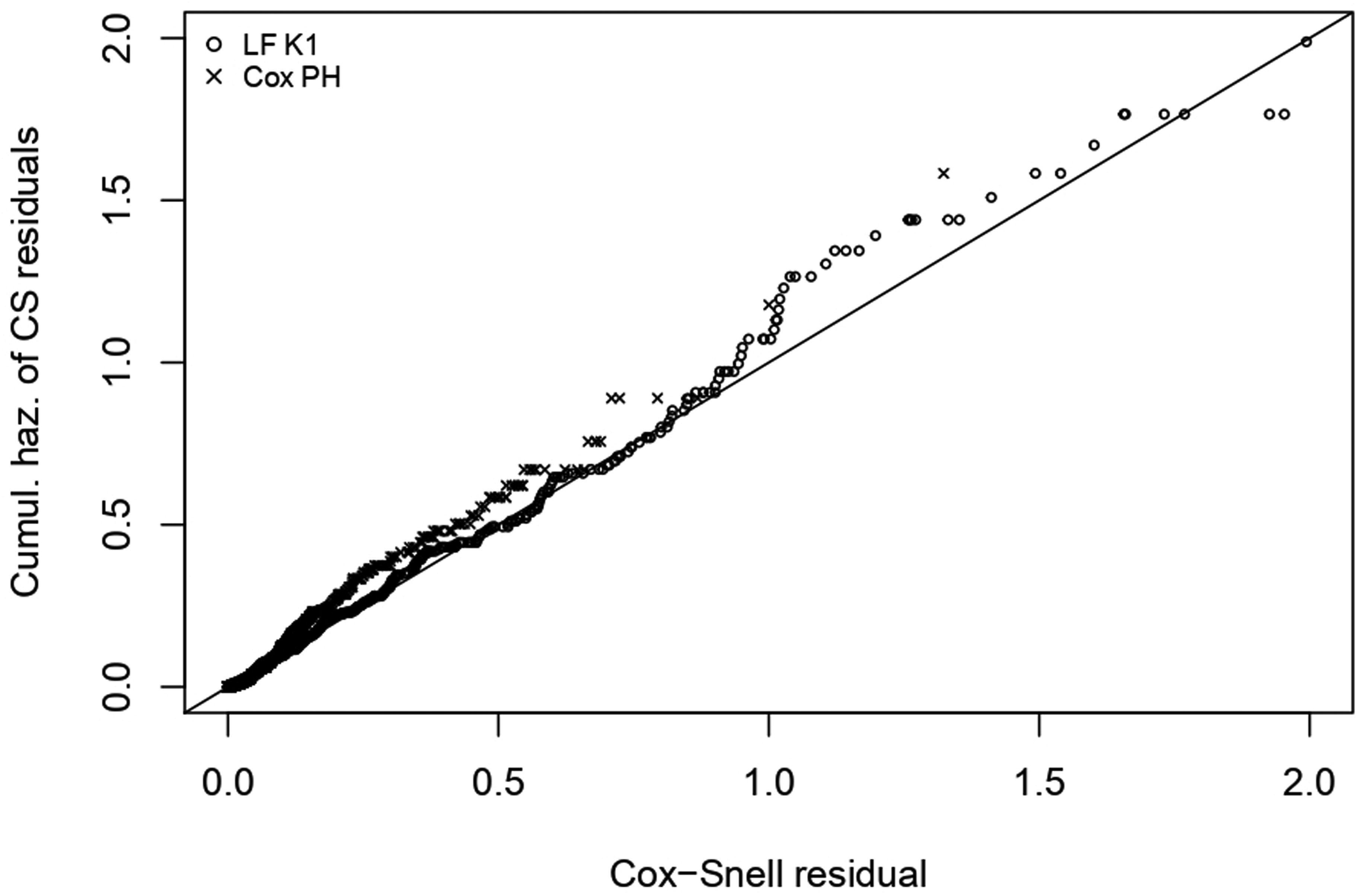
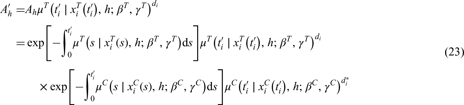
In addition, we compare these two models in terms of goodness of fit, which can help in the choice between these two models. At this purpose we look at the Cox-Snell residuals, $r_i^{CS}$ ( ⁴³ ), defined as the integrated hazard function. A well known result in mathematical statistics states that these residuals have an Exp(1) distribution if the model has been properly specified.

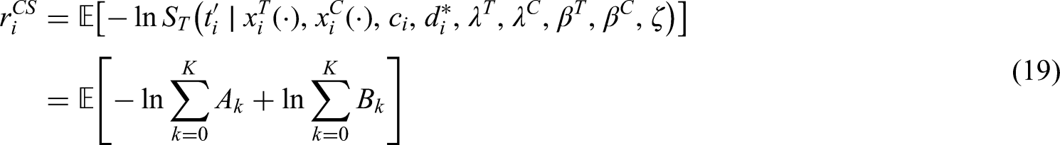
For the Cox PH model, these can be derived as a by product of the estimation process by using the package survival ( ⁴⁴ ), while for the latent factor model of this work, $r_i^{CS}$ is calculated as follows:

$$\begin{array}{rl}{r}_i^{CS}& =\mathbb{E}[-\ln S_T(t_i^{\prime }\mid x_i^T(\cdot ),x_i^C(\cdot ),c_i,d_i^{*},{\lambda }^T,{\lambda }^C,{\beta }^T,{\beta }^C,\zeta )]\\ & =\mathbb{E}[-\ln {\displaystyle \sum _{k=0}^K{A}_k+\ln {\displaystyle \sum _{k=0}^K{B}_k}}]\end{array}$$

(19)

where

$$A_k=\exp [-{\int }_0^{t_i^{\prime }}{\mu }^T(s\mid x_i^T\left(s\right),h;{\beta }^T,{\gamma }^T)\mathrm{d}s]B_k$$

(20)

$$B_k=\exp [-{\int }_0^{t_i^{\prime }}{\mu }^C(s\mid x_i^C\left(s\right),h;{\beta }^C,{\gamma }^C)\mathrm{d}s]{\mu }^C{(t_i^{\prime }\mid x_i^C\left(t_i^{\prime }\right),h;{\beta }^C,{\gamma }^C)}^{d_i^{*}}$$

(21)

In other words, unlike the Cox PH model where we have a point estimate for the integrated hazard function, we average the integrated hazard function for the latent factor model over the draws from the posterior distribution. In addition, since we jointly model the time to event and the censoring time, we need to consider the probability distribution of $T$ conditional on the censoring time (other than the covariates).

In order to check whether $r_i^{CS}$ has Exp(1) distribution, we then calculate the Kaplan-Meier estimate of such residuals, and we plot $r_i^{CS}$ against their Kaplan-Meier estimate of the integrated hazard function, as shown in Figure 2.

Figure 2.

Cox-Snell residuals for the latent factor model with $K=1$ (LF K1, o) and for the Cox PH model (x) plotted against their cumulative (or integrated) hazard function.

We see that the Cox-Snell residuals of the latent factor approach of this work follows more closely the 45-degrees straight line, compared to the Cox PH model, meaning that the former returns a better fit for the distribution of the time to event $T$ .

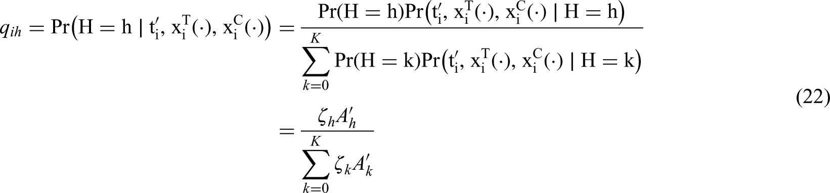
A by-product of this analysis is the possibility to analyse the profile of the two subgroups (since K=1) arising from this modelling approach. Using Bayes’ theorem we can calculate the posterior distribution of $H$ for each patient $q_{ih}$ :

$$\begin{array}{rl}{q}_{ih}=\text{Pr}(H=h\mid t_i^{\prime },x_i^T(\cdot ),x_i^C(\cdot ))& =\frac{\text{Pr}(H=h)\text{Pr}(t_i^{\prime },x_i^T(\cdot ),x_i^C(\cdot )\mid H=h)}{{\displaystyle \sum _{k=0}^K\text{Pr}(H=k)\text{Pr}(t_i^{\prime },x_i^T(\cdot ),x_i^C(\cdot )\mid H=k)}}\\ & =\frac{{\zeta }_h{A}_h^{\prime }}{{\displaystyle \sum _{k=0}^K{\zeta }_k{A}_k^{\prime }}}\end{array}$$

(22)

where

$$\begin{array}{rl}{A}_h^{\prime }=& A_h{\mu }^T{(t_i^{\prime }\mid x_i^T\left(t_i^{\prime }\right),h;{\beta }^T,{\gamma }^T)}^{d_i}\\ =& \exp [-{\int }_0^{t_i^{\prime }}{\mu }^T(s\mid x_i^T\left(s\right),h;{\beta }^T,{\gamma }^T)\mathrm{d}s]{\mu }^T{(t_i^{\prime }\mid x_i^T\left(t_i^{\prime }\right),h;{\beta }^T,{\gamma }^T)}^{d_i}\\ & \times \exp [-{\int }_0^{t_i^{\prime }}{\mu }^C(s\mid x_i^C\left(s\right),h;{\beta }^C,{\gamma }^C)\mathrm{d}s]{\mu }^C{(t_i^{\prime }\mid x_i^C\left(t_i^{\prime }\right),h;{\beta }^C,{\gamma }^C)}^{d_i^{*}}\end{array}$$

(23)

The patient can be hard-assigned to each group by using the Bayes’ rule: let ${\kappa }_i$ denote to which group the patient has been assigned. According to this rule we obtain that ${\kappa }_i=h$ if $q_{ih}\ge q_{ij}$ for $j=0,\dots ,K$ , that is, the patient is assigned to the group for which $q_{i\cdot }$ is highest.

For this dataset we could observe for example that 234 out of 236 censored patients are classified as corresponding to the group with $H=1$ , which is characterized by a lower hazard function for the primary event (since ${\gamma }_1^T<0$ ) and (obviously) a higher hazard for the censoring event. In addition, patients with lower baseline CD4 cell count are more likely to be classified in the group with $H=0$ (mean 345.64 against a mean of 365.28 for $H=1$ ). Further analysis with other covariates are likewise possible. We hereby take into account the CD4 as it is part of the hazard function specification for $T$ and $C$ .

Extensions

Analysis of competing risks

We can extend the approach described so far to the analysis of the joint distribution of $(T_1,\dots ,T_M)$ where $T_j$ is the time to event for the $j$ th cause of decrement ( $j=1,\dots ,M$ ). Within a competing risks framework only $T^{\prime }=\text{min}(T_1,\dots ,T_M)$ can be observed.

Suppose that conditional on the latent factor $H$ , $(T_1,\dots ,T_M)$ is a vector of pairwise independently distributed times to event, whose distribution is characterized by the following hazard function:

$${\mu }^m(t\mid x^m(t),h;{\beta }^m,{\gamma }^m)={\mu }_0^m\left(t\right)\exp ({\beta }^{m^{\prime }}{x}^m(t)+{\gamma }_1^m{h}_1+\dots +{\gamma }_K^m{h}_K)$$

(24)

for $m=1,\dots ,M$

In this way, we can also account for further independence assumptions: for example, if ${\gamma }^m=({\gamma }_1^m,\dots ,{\gamma }_K^m)=0$ , then $T_m$ is independently distributed with respect to the vector $(T_1,\dots ,T_{m-1},T_{m+1},\dots ,T_M)$ .

More generally, instead of having one common latent factor for all competing risks, we can have $H_m$ ( $m=1,\dots ,M$ ), such that the statistical association among time to events is characterized by the joint distribution of $(H_1,\dots ,H_M)$ .

Clustered units

Suppose we deal with units divided into clusters, such as patients in different clinics, each corresponding to a level of the categorical variable $G$ , whose value is known for each patient.

It is possible to account for the specific cluster either by including $G$ as a factor in the hazard function, or by letting $G$ to explain the heterogeneity in the distribution of $H$ for each unit.

In the latter case, we can reasonably assume that $G$ is independently distributed with respect to $T$ and $C$ conditional on $x^T$ , $x^C$ and $H$ . Then, the joint distribution of $(T,C)$ for the $i$ th individual becomes:

$$\begin{array}{rl}& f(t,c\mid x_i^T\left(t\right),x_i^C\left(c\right);{\beta }^T,{\gamma }^T,{\beta }^C,{\gamma }^C)\\ & ={\displaystyle \sum _{k=0}^K\text{Pr}(H=k\mid g_i)[\exp (-{\int }_0^t{\mu }_0^T\left(s\right)\exp ({\beta }^{T^{\prime }}{x}_i^T(s)+{\gamma }_k^T)\mathrm{d}s)}\\ & \times {\mu }_0^T\left(t\right)\exp ({\beta }^{T^{\prime }}{x}_i^T(t)+{\gamma }_k^T)]\\ & \times \left[\exp (-{\int }_0^c{\mu }_0^C\left(s\right)\exp ({\beta }^{C^{\prime }}{x}_i^C(s)+{\gamma }_k^C)\mathrm{d}s)\left({\mu }_0^C\left(c\right)\exp ({\beta }^{C^{\prime }}{x}_i^C(c)+{\gamma }_k^C)\right)\right]\end{array}$$

(25)

This modelling framework allows also to compare clusters. One possibility is the use of the Hellinger distance, which is used for example in topic models to qualitatively compare the topical content of two documents ( ⁴⁵ ). Let $\text{CL1}$ and $\text{CL2}$ be any two different known clusters for the units in the sample: the Hellinger distance $d_H(\text{CL1},\text{CL2})$ is

$$d_H(\text{CL1},\text{CL2})={\displaystyle \sum _{k=0}^K{(\sqrt{\text{Pr}(H=k\mid G=\text{CL1})}-\sqrt{\text{Pr}(H=k\mid G=\text{CL2})})}^2}$$

(26)

When Bayesian techniques are used for inference, as we do in the present work, then the Hellinger distance is given by the expectation of $d_H(\cdot ,\cdot )$ with respect to the posterior distribution of the parameters.

Conclusions

This work illustrated the potential of the use of latent factors to accomodate for the possibility of informative censoring in survival analysis. We rejoined existing literature, and described how we can generalize the specification of the heterogeneity component of the hazard function. We also emphasized how this methodology can be extended to the analysis of competing risks (Section 6.1) and of data from different known clusters (Section 6.2).

The inferential challenges of this type of ill-posed models have been addressed by means of a fully Bayesian approach and we described how modern computational tools such as Hamiltonian Monte Carlo methods are strongly recommended in these circumstances.

We applied those methodologies to the analysis of the ACTG175 clinical trial and we found that modelling the heterogeneity and the presence of informative censoring turns out to improve the model fit in terms of information criterion when compared with standard approaches such as the assumption of non-informative censoring.