Sage Journals: Discover world-class research

Abstract

Multiple different screening tests for candidate leads in drug development may often yield conflicting or ambiguous results, sometimes making the selection of leads a nontrivial maximum-likelihood ranking problem. Here, we employ methods from the field of multiple criteria decision making (MCDM) to the problem of screening candidate antibody therapeutics. We employ the SMAA-TOPSIS method to rank a large cohort of antibodies using up to eight weighted screening criteria, in order to find lead candidate therapeutics for Alzheimer’s disease, and determine their robustness to both uncertainty in screening measurements, as well as uncertainty in the user-defined weights of importance attributed to each screening criterion. To choose lead candidates and measure the confidence in their ranking, we propose two new quantities, the Retention Probability and the Topness, as robust measures for ranking. This method may enable more systematic screening of candidate therapeutics when it becomes difficult intuitively to process multi-variate screening data that distinguishes candidates, so that additional candidates may be exposed as potential leads, increasing the likelihood of success in downstream clinical trials. The method properly identifies true positives and true negatives from synthetic data, its predictions correlate well with known clinically approved antibodies vs. those still in trials, and it allows for ranking analyses using antibody developability profiles in the literature. We provide a webserver where users can apply the method to their own data: http://bjork.phas.ubc.ca.

Keywords

MCDM SMAA-TOPSIS ranking drug development lead optimization Alzheimer’s disease

1 Introduction

Prior to FDA review or clinical development, and before the submission of an investigational new drug (IND) application, pre-clinical research of a new potential therapy must be performed where drug targets are identified and validated, high-throughput screens are performed, candidate therapeutics are identified, and leads are optimized, in order to eventually select a candidate molecule or molecules for clinical development.^1–3

The details of screening methodologies differ between antibody and small molecule drug development. In both cases, however, situations arise where one must choose leads from a large pool of candidates, across multiple screening criteria whose outcomes—addressing physicochemical properties such as binding efficacy, ADME pharmacokinetics, or toxicity—may be ambiguous in the absence of more quantitative analysis.

Large datasets obtained from high-throughput screens^4–7 generally must be post-processed. This is often implemented using graphical statistical tools.^8–10 The above-mentioned ambiguous and sometimes conflicting results that can emerge from multiple screening criteria of small molecules are often cast as a multi-objective optimization/multi-parameter optimization (MPO) problem.^11–15

However, multi-parameter optimization is a specific case of a more broad class of problems known as multiple-criteria decision making (MCDM) problems.^16–18 These problems appear in operations research when one needs to make decisions or rankings by quantitatively evaluating many unrelated, correlated, or conflicting pieces of information simultaneously. MCDM techniques are particularly useful when the multiple measured criteria are not well-correlated with each other but their importance is known, at least approximately, in advance. MCDM problems have been extensively studied and applied in fields such as management,¹⁹ engineering,²⁰ finance and economics,^21,22 energy policy²³ and environmental science.²⁴

MCDM methods can be categorized into two classes based on how different screening criteria are compared: Value-based methods and outranking methods. Value-based methods rank alternative candidates by weighing each of several screening criteria by a user-defined, multiplicative factor; the results are then added up to give a score for each alternative.^25–29 Outranking methods also ascribe a weight to each criterion, but make pairwise comparisons across all candidates, and accumulate criterion-dependent weights for each candidate for each pairwise “win”. A score is given for each candidate by adding the weights corresponding to its wins, and subtracting the weights corresponding to its losses.^16,30–33 One of the most common MPO methods in drug design, Pareto Optimization, is in fact an example of an outranking method.

One significant problem in systematic drug screening is that the multiple criteria used to evaluate a promising candidate are difficult to properly weight by importance or predictive power. When there is uncertainty in the measured values for each criterion, and/or the weighting to be applied to the various criteria is not known exactly, one of two techniques is typically employed: Stochastic Multi-criteria Acceptability Analysis (SMAA),^34–37 or Fuzzy Numbers.^38–42

Here, we introduce MCDM to the problem of ranking drug candidates when multiple screening criteria have been measured to gauge efficacy, and corresponding estimates for appropriate weights ascribed to these criteria have been estimated. These weights need not be known precisely. The method we apply here has historically been called the SMAA-TOPSIS method.^37,43 The “SMAA” component of this method randomizes the weights and/or screening criteria values, and repeatedly re-ranks the candidates to obtain a rank-distribution for each candidate, allowing the candidates to be sorted overall. The “TOPSIS” component refers to the Technique for Order Performance by Similarity to Ideal Solution,^27,44 discussed further below.

In this paper, we apply the SMAA-TOPSIS method to the problem of optimizing the ranking of a set of therapeutic antibody candidates, for their predicted efficacy as potential treatments for Alzheimer’s disease. The multi-criteria optimization problem described below involves either seven or eight screening criteria. We introduce the “retention probability” as the likelihood that a highly-ranked candidate remains highly-ranked upon random changes (errors) in the weights or screening values, and we finally derive a new measure that we call the “topness”, which is related to an integral of the retention probability. We propose the topness and retention probability as best metrics to rank lead candidates for this class of problem. We also validate our results against synthetic data sets, as well as real data sets of antibodies that are either approved or in clinical development.

2 Methods

In this section, we first describe our cohort of candidate antibodies and the multiple screening measurements made to these antibodies which constitute our dataset. We then investigate the correlations between different screening criteria. Next, we derive the TOPSIS method for ranking the antibodies according to a weighted set of screening measurements. We then describe how to account for the uncertainty in these weights, and define the retention probability as well as the topness for ranking the candidates. Next, we describe both our construction of a synthetic dataset and analysis method for a real dataset, in order to validate the method. Finally, we give a flowchart summarizing the steps followed in applying the method.

2.1 Antibody generation and screening criteria

Here we briefly describe the generation of a large set of antibody clones to which the screening and selection method is applied. A previous methodology^45,46 predicted at least five epitopes in Aβ peptide oligomers that would be distinct from either Aβ monomer or Aβ fibril – a desirable condition for an effective Alzheimer’s therapeutic.^47–51 Antibodies were raised to these epitopes by active immunization in mice using subcutaneous aqueous injections containing antigen.⁵² Lymphocytes were then harvested for hybridoma cell line generation. Single cell-derived hybridomas were grown to form monoclonal colonies on semi-solid media. Tissue culture supernatants from the hybridomas were tested by indirect Enzyme-linked immunosorbent assay (ELISA) on screening antigen (the immunized cyclic peptide conjugated to bovine serum albumin (BSA)). This procedure resulted in the generation of 66 candidate antibodies.

The above 66 antibodies were then screened by several methods.^49,53 Binding response units (B) were measured in surface plasmon resonance (SPR) assays against soluble, synthetic Aβ₄₂ oligomers (B_o), soluble Aβ₄₀ monomer (B_m), substrate immobilized Aβ₄₂ oligomers ( $B_{o}^{i}$ ), substrate immobilized Aβ₄₂ monomer ( $B_{m}^{i}$ ), cerebrospinal fluid (CSF) from AD patients ( $B_{A D}^{CSF}$ ), CSF from non-AD patients (control group abbreviated as CTL) ( $B_{CTL}^{CSF}$ ), brain extracts (homogenates) (BH) from AD patients ( $B_{A D}^{B H}$ ), and BH from non-AD patients ( $B_{CTL}^{B H}$ ). For a subset of the antibody clones, immunohistochemistry (IHC) was also performed using frozen human brain sections without fixation or antigen retrieval, and samples were assessed for the absence of overt binding to plaque (B_pla). Low plaque binding was desirable in this development pipeline because plaque binding could cause adverse, dose-limiting effects associated with cerebral edema and microhemorrhages. To reflect the more qualitative nature of the IHC measurements, B_pla was ascribed discrete values. Values obtained from the above measurements are listed in supplemental Table S1.

Screening of IgG clones raised against the distinct Aβ oligomer epitopes allows us to rank the antibodies by using the following desired profile, corresponding to eight screening criteria. Screening variables here are represented in terms of binding B in an SPR assay. (1) Selective/relative binding to synthetic oligomers vs. monomers, both in solution, and when immobilized in SPR assays, (2) Relative binding by SPR to native soluble Aβ oligomer in CSF and Brain extracts of AD patients, minus binding in non-AD control patients, (3) Absolute SPR binding to oligomer in CSF and brain extract of AD patients (without subtracting binding to non-AD patients), (4) Absolute binding to immobilized oligomer (without subtracting monomer affinity), (5) Lack of plaque reactivity by IHC on unfixed AD brain sections. The above criteria are thought to characterize an effective AD antibody therapeutic.^48–51

The measurements corresponding to the above criteria correspond to eight variables: $B_{o} - B_{m}, B_{o}^{i} - B_{m}^{i}, B_{A D}^{CSF} - B_{CTL}^{CSF}, B_{A D}^{B H} - B_{CTL}^{B H}, B_{A D}^{CSF}, B_{A D}^{B H}, B_{o}^{i}, B_{pla}$ . Plaque binding values are normalized to be between 0.5 and 1 as described below. For all other criteria, we normalized the measurement to lie within the range $[0, 1]$ by using the formula

B_{norm} = \frac{B - B_{min}}{B_{max} - B_{min}}

(1)

where B_max and B_min are the maximum and minimum values observed for each of the corresponding criteria, respectively. By construction, a higher value of B is better for all screening criteria. This procedure places all of the criteria on equal footing after normalization (but before unequal weighting). To simplify the notation, we label the eight normalized criteria as B_i (i = 1

\dots

8).

In our IHC assay, no or low plaque binding was a favorable criterion. Because the IHC plaque binding measurement is simply classified as “+”, “−” and “ $+ / -$ ” (the latter indicating weak or heterogeneous binding), we assigned values of 0.5, 0.75 and 1 to +, $+ / -$ , and −, respectively. Measurements from 2 brain samples were averaged to give overall numbers ranging from 1, 0.875, 0.75, 0.625, and 0.5, which appear in supplemental Table S1.

2.2 Determining the independence of different screening criteria

A promising drug candidate should perform well for each of the eight criteria mentioned above; likewise a poor candidate should not outperform a good candidate for many of the criteria. The performance of a given candidate across the above criteria may thus be expected to correlate to some degree. On the other hand, if the data for two different criteria were perfectly correlated, they would then be redundant and could be reduced into one single criterion. Generally, each new screening criterion adds new information, so that the screening values may be moderately correlated with those from previous criteria, but with scatter, so that each criterion adds new information. Figure 1(a) shows a color-coded table of the correlation coefficients between all pairs of screening measurements for our dataset. The last column/row corresponding to B_pla was calculated from the 26 antibodies with B_pla data available; all other correlations used the full cohort of 66 antibodies. Measurements are grouped in Figure 1 using k-means clustering⁵⁴ (see Supporting Information for the clustering method).

Figure 1.

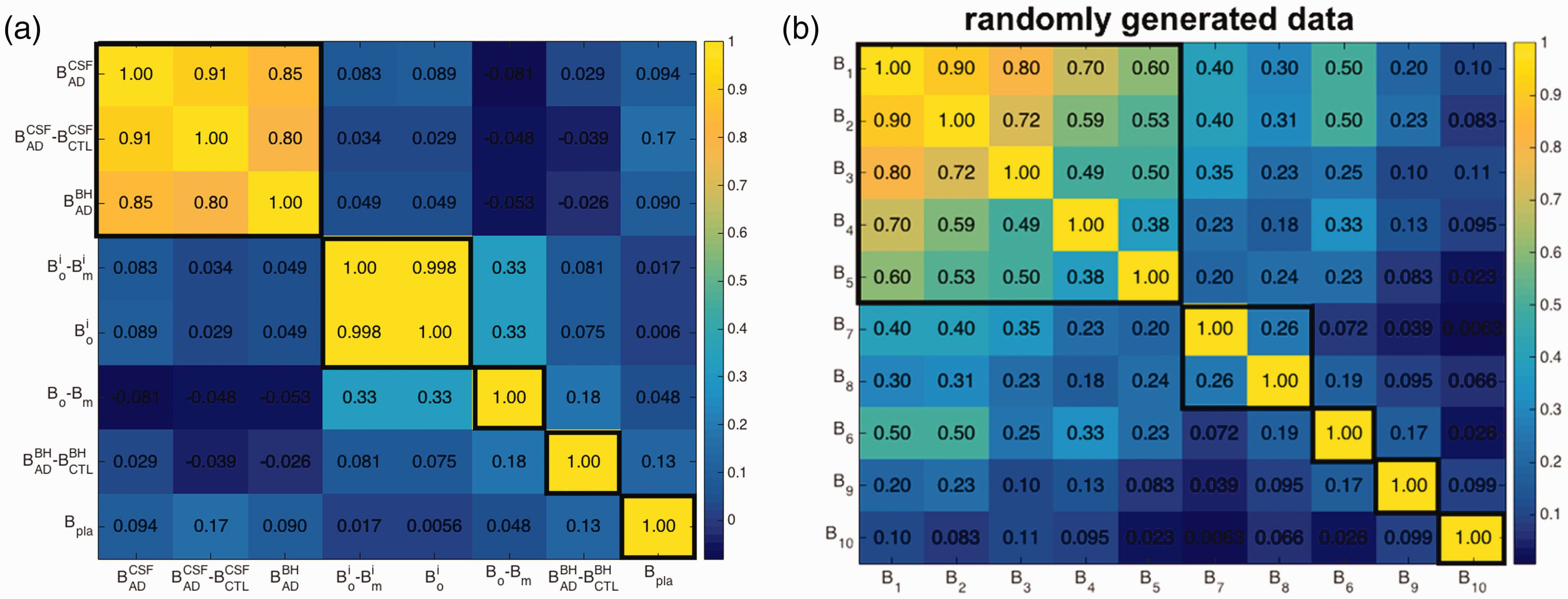
Color coded table of correlation coefficients between all pairs of screening criteria, (a) for the binding response unit dataset of our antibodies, (b) for a synthetic dataset described in the text. Thicker black lines outline k-means clusters determined so that all members within a cluster are significantly correlated. Note that in (b), screening criteria are indexed according to their correlation coefficient with B₁ (e.g. B₅ and B₁ have correlation 0.6, B₆ and B₁ have correlation 0.5 and so on, but they are sorted in panel (b) according to their k-means clustering, which places criterion B₆ out of order.

Figure 1(a) shows that several pairs of measurements are essentially uncorrelated, e.g. $B_{A D}^{B H} - B_{CTL}^{B H}$ and $B_{o}^{i}$ . Other measurement pairs, such as $B_{o}^{i}$ and $B_{o}^{i} - B_{m}^{i}$ , have correlation coefficient close to unity, in this case because the quantity $B_{m}^{i}$ is always much smaller than $B_{o}^{i}$ (see Supplemental Table S1). Such strongly correlated quantities will add little new information in the analysis; one utility of the correlation matrix is then in revealing potential pairs of measurements that may be consolidated. Here, we retain both $B_{o}^{i}$ and $B_{o}^{i} - B_{m}^{i}$ as there is no harm in keeping both, but we reduce the weights of the two strongly correlated measurements (giving $B_{o}^{i}$ the smallest initial weight), since they account for essentially the same information. The weights for each quantity are discussed below in Section 2.4 and given in Table 1. It is finally worth noting that the fact that the measures in Figure 1(a) often do not correlate with each other makes the problem of deciding the top candidates non-trivial, and potentially dependent on the relative importance of the different screening criteria.

Table 1.

The criteria for evaluating antibodies and their corresponding initial weight w_i before errors are accounted for.

Criteria	$B_{o} - B_{m}$	$B_{o}^{i} - B_{m}^{i}$	$B_{A D}^{CSF} - B_{CTL}^{CSF}$	$B_{A D}^{B H} - B_{CTL}^{B H}$
w_i	0.5	0.5	1	1
σ_i	$\frac{0.5}{\sqrt{3}}$	$\frac{0.5}{\sqrt{3}}$	0.5	0.5

Criteria	$B_{A D}^{CSF}$	$B_{A D}^{B H}$	$B_{o}^{i}$	B _pla
w_i	0.5	0.5	0.25	1
σ_i	$\frac{0.5}{\sqrt{3}}$	$\frac{0.5}{\sqrt{3}}$	$\frac{0.25}{\sqrt{3}}$	0.5

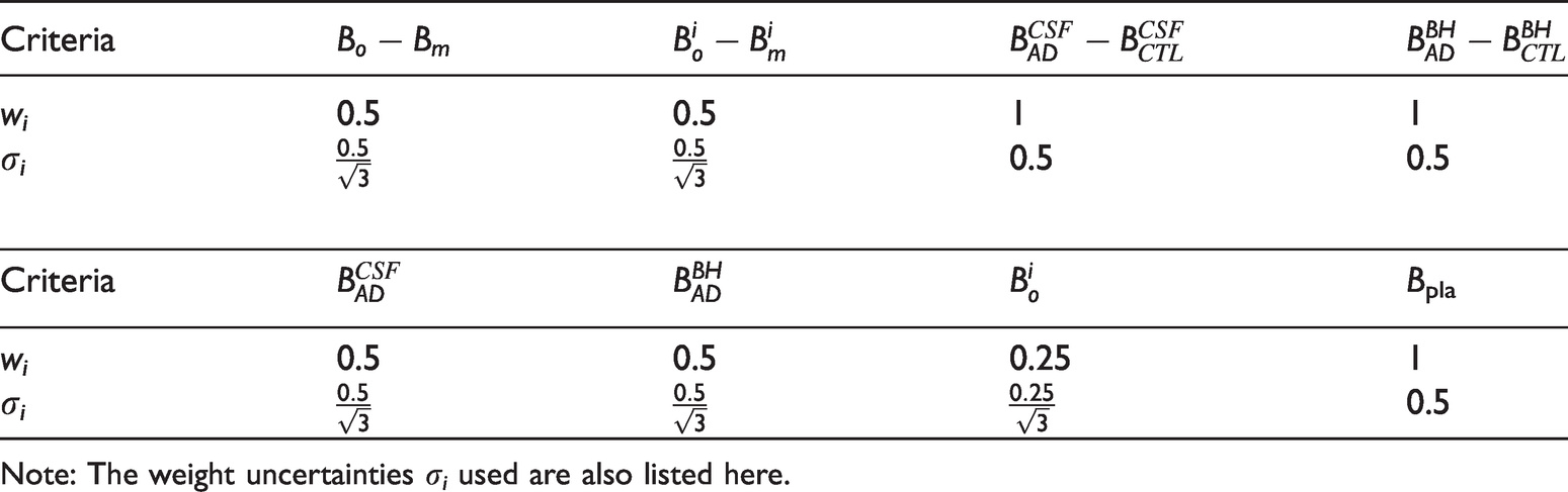
Note: The weight uncertainties σ_i used are also listed here.

2.3 TOPSIS method in Hilbert space, for ranking drug candidate performance

We now describe how we use the above eight criteria to screen for promising antibody candidates. The eight criteria constitute an eight-dimensional (8 D) vector space (i.e. a Hilbert space), with the binding profile $\vec{B} = {B_{i}}$ $(i = 1$ … $8)$ for each antibody representing one point in this 8 D-space. Because of the normalization in equation (1), the origin corresponds to a hypothetical antibody with values {B_min} for all eight criteria. Ranking the antibodies then amounts to sorting them by a quantity similar to their distance in 8 D-space between the antibody-points and the origin, $\sqrt{\sum_{i = 1}^{8} B_{i}^{2}}$ .

An additional feature is important to include in the analysis, however: Not all screening criteria have equal importance, and correspondingly, they should be given different weights. Often though, we don’t know exactly what these weights should be. Let our best guess for the weight of measurement i be w_i, and let the corresponding weighted scalar distance used in determining the performance quality of a drug candidate be given by 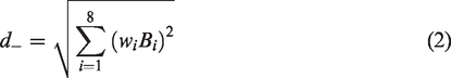$w_{i} B_{i}$ . A measure in the 8 D Hilbert space of the quality of a drug candidate is then

d_{-} = \sqrt{\sum_{i = 1}^{8} {(w_{i} B_{i})}^{2}}

(2)

where w_i is the weight of the i-th criteria and B_i is the normalized criterion we listed above. A larger radius represents a better performing and thus more promising drug candidate. In the language of TOPSIS, the origin corresponds to the ideal worst solution (IWS),²⁷ i.e. the coordinates of the worst possible performing candidate:

{w_{i} B_{i}^{min}} = {0, 0, \dots 0}

. The above 8 D weighted radius,

d_{-}

in equation (2), is thus the distance from the IWS.

In the TOPSIS approach, the distance from the ideal best solution (IBS) plays nearly as important a role as the distance from the IWS. The IBS has coordinates 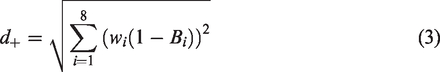${w_{i} B_{i}^{\max}} = {w_{1}, w_{2}, \dots w_{8}}$ , so the Euclidean distance from the IBS is

d_{+} = \sqrt{\sum_{i = 1}^{8} {(w_{i} (1 - B_{i}))}^{2}}

(3)

A smaller 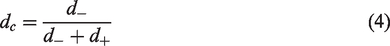$d_{+}$ would imply a more promising candidate. The TOPSIS method ranks on the fraction of the total distance $(d_{-} + d_{+})$ that arises from $d_{-}$ , referred to as “the relative closeness”^27,37,43,44

d_{c} = \frac{d_{-}}{d_{-} + d_{+}}

(4)

The closeness d_c is a nonlinear function of the distances $d_{-}$ and $d_{+}$ . Other functions may also be used to rank candidates, e.g. ranking on the more symmetrical quantity $(d_{-} - d_{+}) / (d_{-} + d_{+})$ is equivalent to ranking on d_c, since the former is simply $2 d_{c} - 1$ .

2.4 Accounting for the uncertainty in measurements and measurement weight when ranking lead candidates

Each of the measurements B_i is generally subject to uncertainty; the error on each B_i thus results in some uncertainty in the resulting ranking. To account for the influence of measurement error on the candidate rankings, we add to each screening value a Gaussian-distributed random number with zero mean and standard deviation corresponding to the experimental error. The error may vary measurement to measurement.

Additionally, the weights w_i reflect intuitive judgments on the importance of the different screening criteria, and thus the effects of errors in w_i must also be treated. Initial guesses for the weights of the various screening measurements are given in Table 1.

Because the weights are uncertain, we determine the sensitivity of the ranking due to variations in the weights by applying uniformly distributed noise to vary each weight. That is, we randomize the weight values according to

w_{i}^{rand} = w_{i} + σ f_{i}

(5)

where f_i is a random number chosen from a uniform distribution centered on w_i, with bounds such that the standard deviation is σ, i.e. half-width

= \sqrt{3} σ

. Since the distribution of weights must contain only positive values, the mean and the standard deviation cannot be independently chosen for all σ. It is straightforward to implement this dependence for a uniform distribution: For a given mean w_i, the maximal width of the distribution is from 0 to

2 w_{i}

, giving an upper bound

σ_{max} = w_{i} / \sqrt{3}

(see Supplemental Figure S1). The randomized weights

w_{i}^{rand}

in equation (5) are now uniformly distributed with mean w_i and standard deviation

σ \leq σ_{max}

In our analysis, we adopt the uncertainty value of $\min (σ_{max}, 0.5)$ for each screening criterion (see Table 1). In principle, however, the confidence or equivalently σ can vary between criteria. Supplemental Figure S1 shows three different weight distributions, with initial values w_i of 0.25, 0.5, and 1, with corresponding standard deviations $σ = 0.25 / \sqrt{3}, 0.5 / \sqrt{3},$ and 0.5, respectively.

There may also be cases when the uncertainty in weights are correlated between criteria, e.g. two weight factors may both be uncertain, but when one is large the other is also expected to be large, and when one to small the other is also expected to be small. This can be accounted for, in principle, by constructing a matrix of correlation coefficients, and generating noise from the corresponding multivariate distribution. However, the correlation coefficients would not be known a priori, and so would themselves be subject to uncertainty. We do not pursue this issue further here.

If measurement noise is present, it is applied as described above, and screening criteria are normalized as before. Weights are then sampled from a random distribution as described above, and criteria are multiplied by their corresponding weights. We then again obtain the rank distributions for the antibodies using the SMAA-TOPSIS method, and finally obtain the ranking of the candidates by calculating the retention probability and topness, as defined in section 2.5. For our dataset, we assumed error bars of 10% on all measurements. Supplemental Figure S2 shows that there are only minor differences in the retention probability p₁₀ (see below for definitions) for our data with and without 10% noise.

2.5 Calculating retention probability and topness

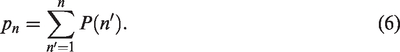
Because there is uncertainty in both the screening values and the weights applied to those values, the ranking (an integer n) of an antibody candidate obeys a distribution P(n). We further define the retention probability, p_n, as the probability an antibody candidate is retained within the top n candidates when uncertainty in both the screening values and weights are present. p_n is thus the cumulative (sum or integral) of P(n) from the 1st to the nth candidate ranking:

p_{n} = \sum_{n' = 1}^{n} P (n') .

(6)

The topness t_n for a given candidate is defined as

t_{n} = \sum_{m = 1}^{n} p_{m},

(7)

where p_m is the top-m retention probability. The topness t_n in equation (7) can be thought of as an integral or cumulative of the retention probability over the top n candidates (and thus a double cumulative of the ranking distribution).

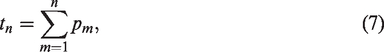
Topness only gives new information when considering the top-n best performing candidates with n less than the total number N. The ranking obtained using the topness over all the candidates, t_N, is equivalent to ranking the candidates by their mean ranking. To see this, note that the mean ranking of an antibody is $\bar{n} = \sum_{n = 1}^{N} n P (n)$ , where P(n) is again the ranking probability distribution. Since the retention probability is the cumulative probability a candidate is ranked in the top n, $p_{n} = \sum_{n^{'} = 1}^{n} P (n')$ , the topness t_n when n = N (the total number of antibodies) is thus $t_{N} = \sum_{n = 1}^{N} \sum_{n^{'} = 1}^{n} P (n') = \sum_{n = 1}^{N} \sum_{n^{'} = 1}^{N} Θ (n \geq n') P (n')$ , where $Θ (n \geq n')$ is the discrete Heaviside function which is unity when $n \geq n'$ and zero otherwise. Switching the order of the sums we have $t_{N} = \sum_{n^{'} = 1}^{N} P (n') \sum_{n = 1}^{N} Θ (n \geq n') = \sum_{n^{'} = 1}^{N} P (n') (N - n' + 1) = N + 1 - \bar{n}$ . Specifically, when an antibody is top ranked on average ( $\bar{n} = 1$ ), t_N = N, which is the largest value the topness can achieve. Thus, when topness is summed over all candidates rather than a subset of them (e.g. the top 5 or top 10), ranking by decreasing order of topness is equivalent to ranking by the mean of the ranking distribution.

On the other hand, the topness method is particularly suitable for selecting lead candidates, when we are not interested in poorly performing candidates. Here, we typically calculate t₁₀.

To rank all antibodies using topness, we start by finding the top 10 antibodies by calculating t₁₀ and sorting. We then remove these antibodies from the list, and iteratively repeat the process, finding the next top 10 antibodies from those remaining, until all antibodies have been ranked.

2.6 Generation of a synthetic validation dataset

To test the method on a synthetic dataset, we generated hypothetical data for 100 candidates (e.g. antibodies) with 10 screening criteria. The correlated screening criteria values are randomly generated from a Gaussian distribution with mean value 0 and standard deviation 1 as described below, and they are then given “correct” initial weights ${w_{i}^{0}}$ by randomly selecting 10 numbers from a uniform distribution having an arbitrary range [0.25, 1]: Here, these weights are {0.30, 0.62, 0.45, 0.42, 0.65, 0.68, 0.43, 0.59, 0.27, 0.87}. Once selected, the values ${w_{i}^{0}}$ are fixed for the rest of the analysis. Correlated data are generated such that the correlation between the data for the first screening criterion B₁ (randomly selected) and the rest, B₂, B₃, $\dots$ , B₁₀, take the values 0.9, 0.8, 0.7 $\dots$ 0.1, respectively (see the top row or 1st column of Figure 1(b), which may be compared with Figure 1(a)). We achieve this by first ascribing 10 randomly generated numbers from Gaussian distribution with mean value 0 and standard deviation 1 for each antibody candidate. Then, noting that these 10 numbers constitute a 10-dimensional vector space, we select a random vector direction in this space. The projection of each antibody coordinate on this vector is taken to be B₁. We then generate an orthogonal vector $B_{⊥}$ , by choosing another random vector in the 10-D space and subtracting the component of B₁ from that vector. The coordinates or screening values along $B_{⊥}$ have zero correlation with B₁. We can then choose a linear combination, $α B_{1} + (1 - α) B_{⊥}$ as a new direction, choosing the mixing coefficient to generate a desired correlation coefficient between B₁ and $B_{2} \dots B_{10}$ . Other schemes are of course possible for generating a correlated set of data.

The generated screening data have correlation matrix shown in Figure 1(b). In the analysis below for this synthetic data, we consider errors in the above weights by choosing weights randomly from a uniform distribution having standard deviation $σ = \min (σ_{max}^{i}, 0.5)$ where $σ_{max}^{i} = w_{i} / \sqrt{3}$ with w_i the above initial values for the weights.

2.7 Summary of the method

In summary, the procedure we have developed here is in practice simple and straightforward to implement, and is shown in the flowchart of Figure 2. After collecting screening data across criteria, give each criterion an estimate for what its weight should be, depending on one’s best guess for that criterion’s importance. Next, choose an estimate for the uncertainty in those weights—this measure can be subjective and depends on the user’s confidence in the weights.

Figure 2.

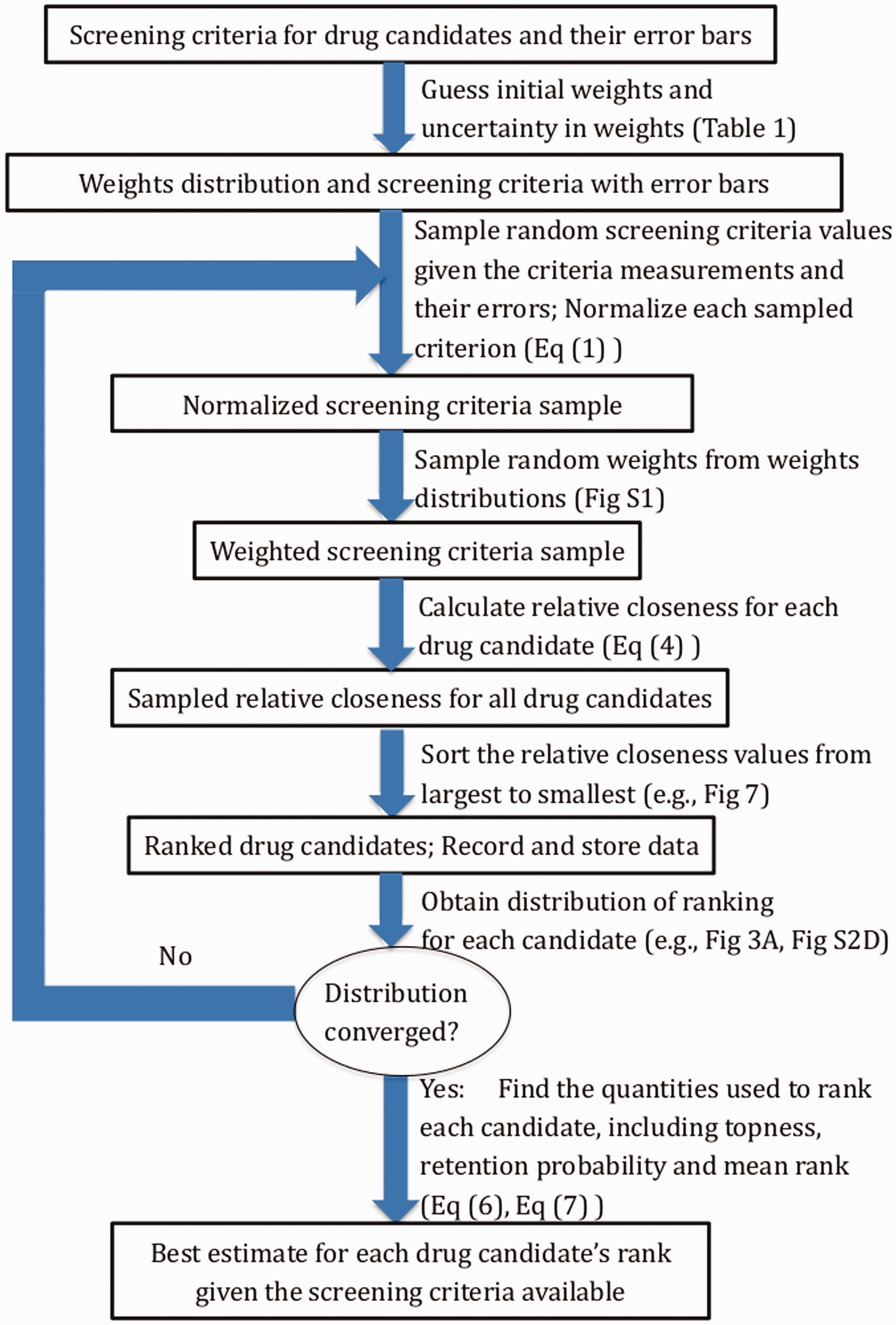
Flowchart of the ranking method. Detailed descriptions for each of the steps are given in Sections 2.3–2.5, and representative tables, figures, or equations are given for each step. The convergence check is described in Supplemental Material Section “Convergence Analysis”. The formula for relative closeness is given in equation (4). To obtain the distribution of ranking for each candidate, we collect the ranking results from all iterations and apply to each candidate.

Next, if there is measurement error to be accounted for (as determined by the measured variance of screening values for each criterion), for the purposes of ranking we then sample the screening criteria values from a Gaussian distribution with appropriate mean and variance.

For each screening criterion, we then normalize each sampling of all the corresponding screening values so that the largest value is unity. The weight values for each criterion are then sampled from a uniform distribution, which has a mean (the best guess) and variance that the user decides, and which may depend on the criterion. These weights then multiply their corresponding normalized criteria, to finally give all of the weighted screening criteria values. By repeatedly sampling the weighted screening values, we repeatedly rank-order the drug candidates according to the relative closeness to the ideal best solution (IBS) and ideal worst solution (IWS) in equation (4), to obtain a converged ranking distribution P(n), a retention probability p_n, (equation (6)) and topness t_n (equation (7)) for each antibody candidate.

3 Results

3.1 Distribution of lead-candidate rankings

We start by applying the stochastic method described above to the weights of the first seven screening criteria B_i ( $i = 1 \dots 7$ ) for all 66 antibodies. A new set of weights for the screening criteria is given by a new set of seven values of w_i obtained after applying uniform noise with $σ = \min (w_{i} / \sqrt{3}, 0.5)$ , as listed in Table 1. Measurement noise of 10% is also applied to all measurements, as described in section 2. Rank-ordering by the closeness in equation (4) then gives a new ranking of the antibodies, from 1st to 66th in our case. The ranking of each antibody candidate according closeness is recorded, and the weight and value distributions are sampled once again to obtain another ranking. This process is repeated until a converged histogram of the ranks is obtained for each antibody candidate. Supplemental Figure S3 shows that these distributions converge after several thousand iterations. Histograms of the rank for 10 arbitrarily selected antibody candidates are shown in Figure 3(a). The initial rank (the rank found from the initial set of weights), the mean rank after randomizing the weights, and the rank by topness are all given in Figure 3(a).

Figure 3.

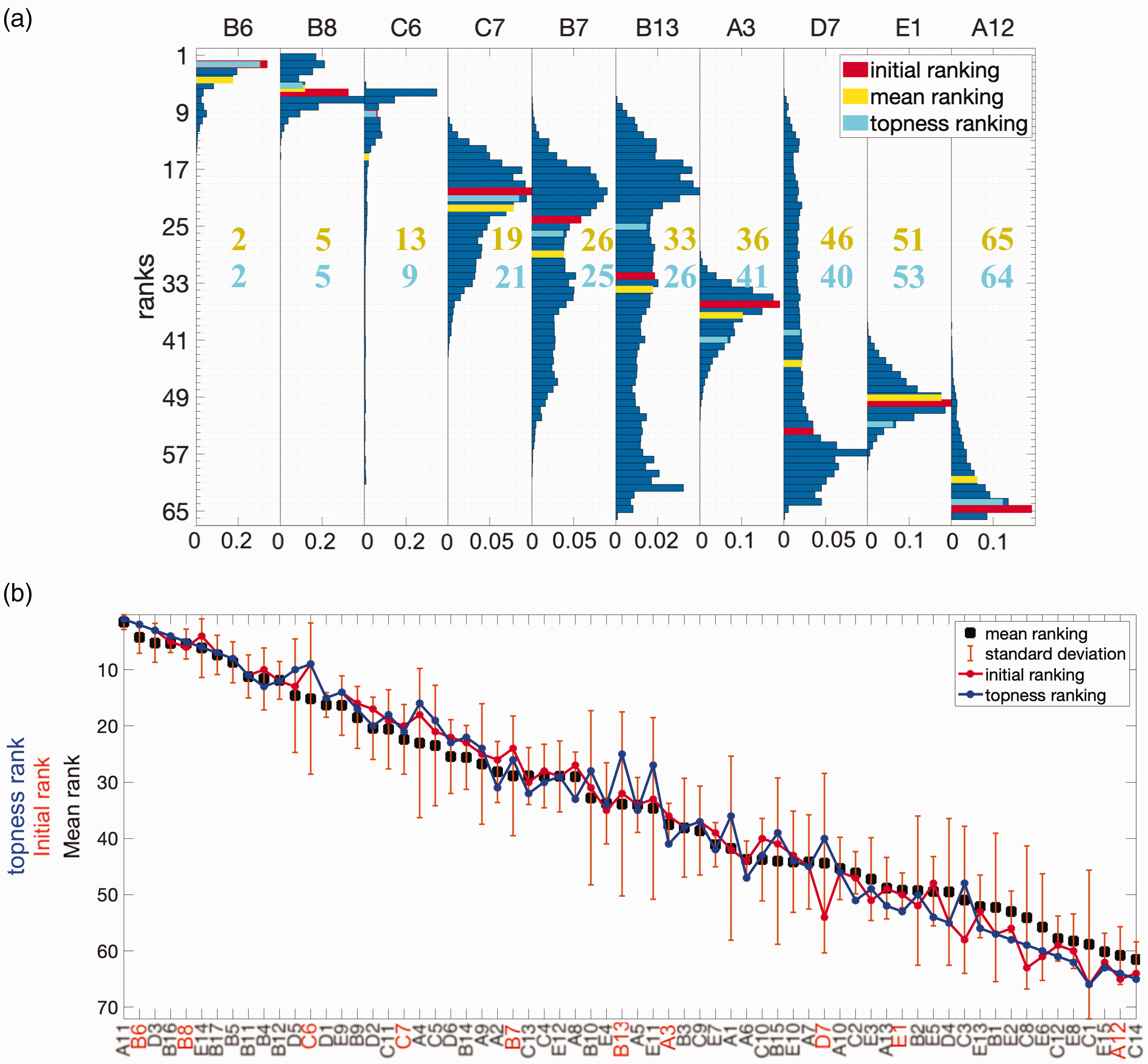
Ranking distributions for selected antibodies and average ranking for all 66 antibodies (a) Ranking distributions for 10 selected antibodies, with weights randomized using $σ = \min (σ_{max}, 0.5)$ with $σ_{max} = w_{i} / \sqrt[]{3}$ , see text). Red histogram bars indicate the initial ranking before randomization, while yellow histogram bars indicate the mean value of the rank distribution. The rank for each antibody as obtained by sorting the mean values highest to lowest is labelled in yellow in each panel, and the rank for each antibody as obtained from the topness (see text) is labelled in cyan (see supplemental Table S1, column 12). (b) The ranking for the 66 antibodies considered here, sorted by the means of the rank-distributions. The “error” bar on each antibody represents the standard deviation of the ranking by randomizing the weights using $σ = \min (σ_{max}, 0.5)$ . The thin red line indicates the ranking of each antibody using our initial guess w₀ for the criteria weighting. The thin blue line indicates the ranking of each antibody using the topness. Antibodies shown in panel (a) are labeled in red font.

For some antibodies, the mean and initial rank coincide; for other antibodies, they differ substantially – see, for example, the red and yellow bars in Figure 3(a). The ranking of a candidate after weight randomization may increase or decrease, depending in a non-trivial way on that candidate’s performance profile across multiple criteria. The overall ranking by mean of the distribution is a nonlinear function of the screening measurements and their weights.

In Figure 3(b), we plot the ranking of the 66 antibodies according to several metrics. The antibodies are sorted on the x-axis from highest to lowest according to the means of their ranking distributions. The standard deviation of the ranking distribution for each antibody, due to randomization of the weights, is shown as error-bars in Figure 3(b). In many cases, the variance in the ranking is significant, which can alter the ranking for different choices of weights. This observation supports further analysis into ranking schemes that go beyond the distribution mean, and account for these fluctuations. Robustness in the ranking is desired, and is quantified through the retention probability and topness, described further below.

The mean rankings in Figure 3(b) need not be integers (and need not be a number as large as 66), since they are averaged over the ranking distribution. The rankings obtained from the initial guesses for the weights are shown by the thin red line in Figure 3(b). Convergence analysis of the mean rank, median rank, and topness is described in Supplemental Section S3 and Supplemental Figure S3.

3.2 Retention probability and topness

Some antibodies in Figure 3(b) have well-defined ranking given uncertainties in weights (e.g. A3, E1, E7), but are not ranked highly. Other antibodies are ranked fairly highly, but have large uncertainties in their ranking given uncertainties in their weights (e.g. C6). To find both highly ranked and robust candidates, we calculate the retention probability for each antibody: the probability that an antibody is retained in the top-n ranked candidates when the weight suffers from uncertainty (see section 2). Figure 4(a) shows the rank-ordered retention probability for an antibody to be within the top 10 candidates, for all antibodies for which this probability is nonzero. 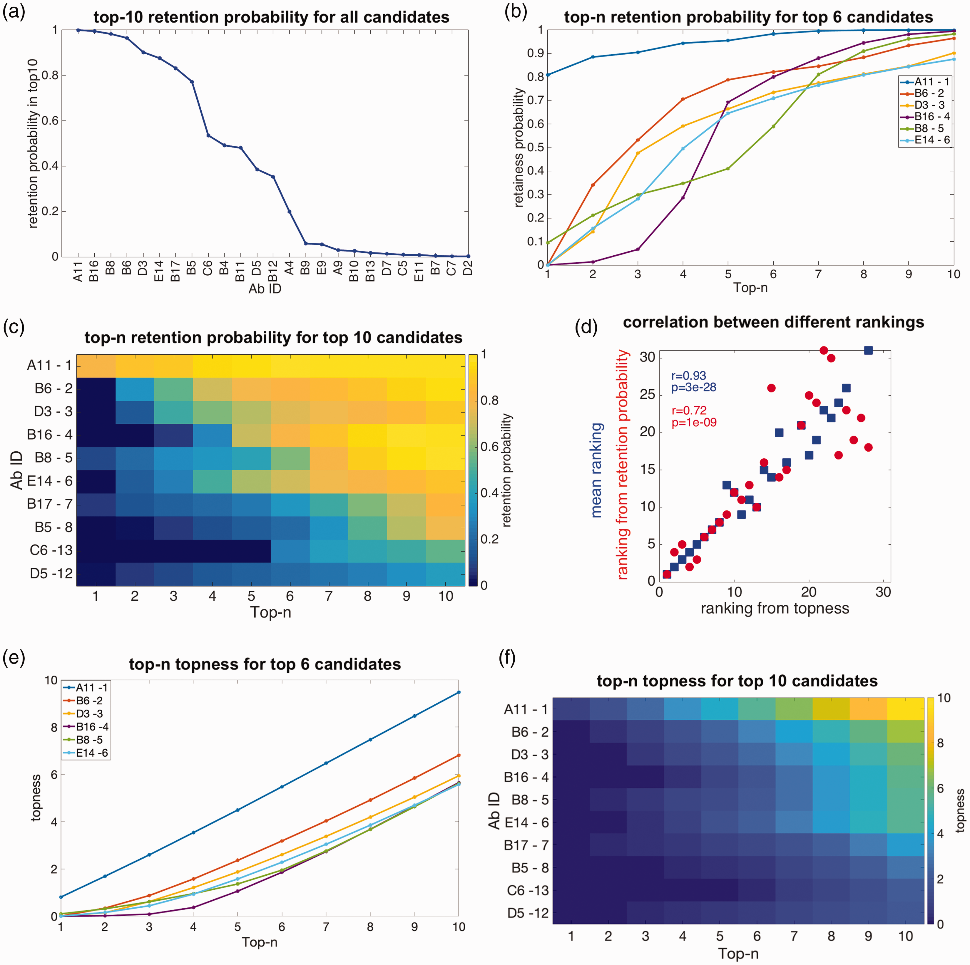The weight uncertainty here is $\min (σ_{max}, 0.5)$ for each screening criterion.

Figure 4.

Retention probability, topness, and correlations between metrics: (a) the top 10 retention probability for all antibodies for which this quantity is nonzero. (b) Retention probability to be in the top-n candidates, as a function of n, for the top six antibodies ranked according to topness. (c) Retention probability from top 1 to top 10 for the top 10 antibodies as ranked by the topness t₁₀. For the top six antibodies, this panel shows the same information as panel (b). The mean ranking is also listed after each antibody ID, for comparison. (d) Two scatter plots: Ranking by top 10 retention probability vs. topness (red); ranking by the mean vs. topness (blue). Kendall’s tau correlation coefficient and significance are given in the legend. (e) Topness as a function of n, for the top six antibodies as ranked by topness t₁₀. (f) Topness from t₁ to t₁₀, for the top 10 antibodies ranked by topness t₁₀.

For each antibody, we can calculate its retention probability to be (in) the top candidate p₁, the top 2 candidates p₂, up to its retention probability to be in the top 10 candidates, p₁₀. In Figure 4(b), we show the retention in top-n probability curve as a function of n, i.e. p_n vs. n for six antibodies.

From the probability of retention in the top m candidates p_m, we define the topness, $t_{n} = \sum_{m = 1}^{n} p_{m}$ , as described in section 2 (see equation (7)). The topness t_n can be thought of as the cumulative probability a given candidate is retained within the top m candidates, as m is progressively increased from 1 to n (moving rightward in Figure 4(b)). So for example, according to Figure 4(b), $t_{4} (A 11) > t_{4} (E 14) > t_{4} (B 16)$ , but $t_{10} (A 11) > t_{10} (B 16) > t_{10} (E 14)$ . Figure 4(c) shows the top-n retention probability p_n as a function of n, for the top 10 candidates as ranked by the topness t₁₀.

In Figure 4(d) we show a scatter plot of the ranking determined by the retention probability p₁₀ vs. the ranking determined by the topness t₁₀, as well as the mean ranking (equivalent to t₆₆) vs. t₁₀. The various ranking methods are correlated with each other, but each conveys different information.

From either Figure 4(b) or 4( c), it is clear that candidate A11 is the top-ranked candidate. Other candidates show interesting cross-over behavior: For example, antibody B6 has zero probability to be the top candidate, but has a good chance to be in the top-2, top-3 and so on, and so is ranked second by topness. On the other hand, for about 7% of the possible weighting parameters, B8 could be the top candidate, but more commonly it does not perform particularly well, and so is ranked fifth. Supplemental Figure S4 shows that the antibody ranking by topness is nearly independent of the distribution (uniform, log-normal, or a positive-definite Gaussian variant) used to choose the values of the weights.

3.3 Sensitivity to the degree of uncertainty in the weights

The data in Figure 3(b) shows that the mean ranking, after averaging over the weights for the various screening criteria, correlates very strongly with the ranking obtained using our initial guesses for the weights. One appropriate way to measure this correlation is through Kendall’s tau coefficient (τ), which measures the similarity of the orderings of two sets of data when ranked by each of the respective quantities.⁵⁵ Here, the Kendall’s correlation between the mean and initial rankings is $τ = 0.95, p (τ) = 3$ e-29.

The error bars in the rankings of Figure 3(b) indicates that, if we were unsure of our initial weightings (to a degree characterized by $σ = \min (σ_{max}, 0.5)$ in equation (5)) and had chosen a different set of ${w_{i}}$ , we could have arrived at a quite different rank-ordering of the antibodies. To quantify how different, we re-sample from the above uniform weight distributions (Supplemental Figure S1), and repeatedly obtain sets of rankings for the 66 antibodies.

Each of these rankings is then compared to the ranking as obtained from the initial guess for the weights, by calculating the Kendall’s τ coefficient. The distributions of τ values and their corresponding statistical significance p are given in Figure 5. These histograms show that the correlation between the rankings obtained from the initial guesses and the randomized weights is always statistically significant, although the degree of correlation can vary. 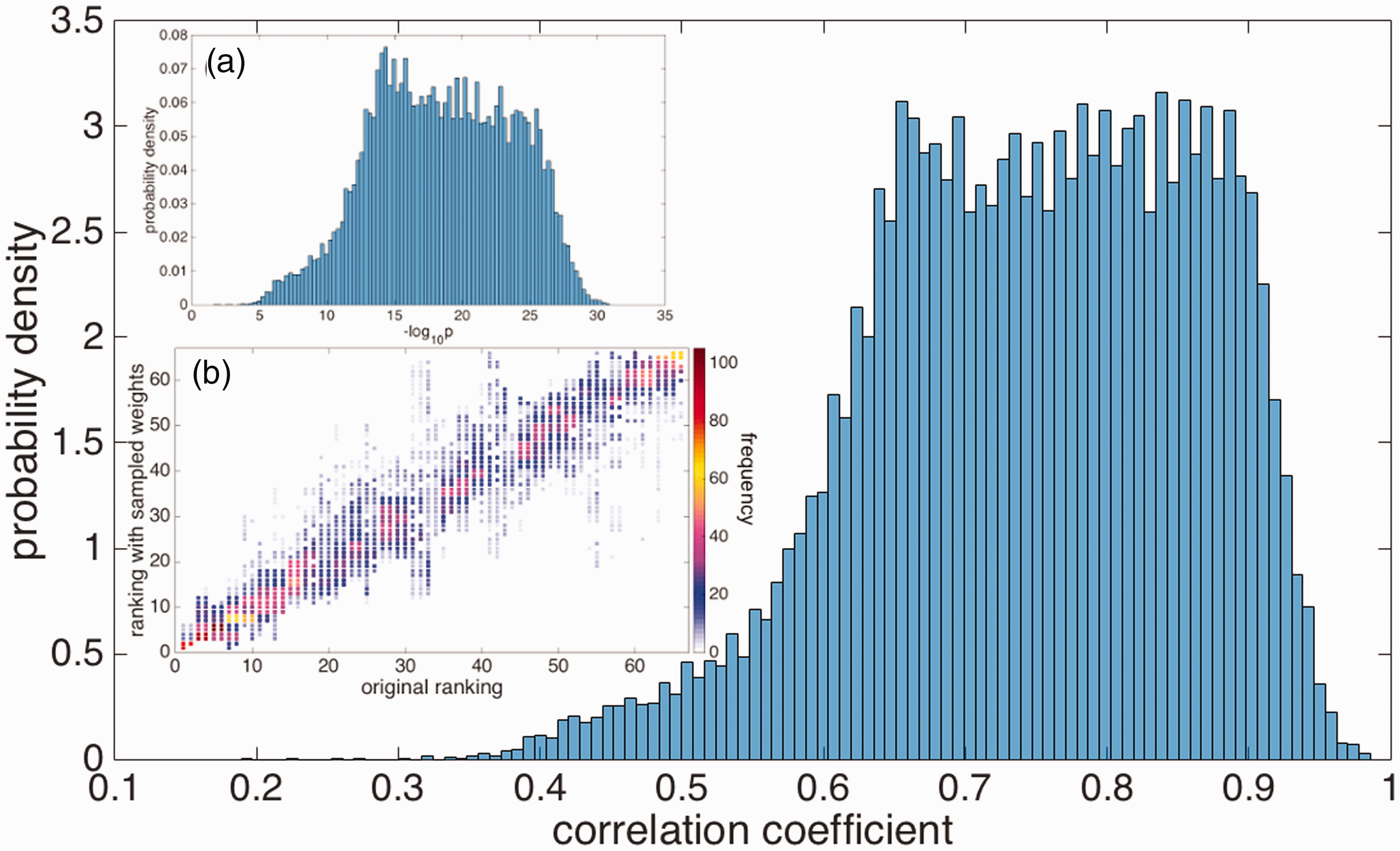The mean values of ( $< τ >, < - \log_{10} p >$ ) over the randomized weights are (0.75, 19).

Figure 5.

The distribution of Kendall’s τ correlation coefficients between the antibody rankings using randomized weights with $σ = \min (σ_{max}, 0.5)$ , and the initial ranking using ${w_{0}}$ . Inset (a): The corresponding distribution of (minus) the logarithm of the statistical significance (p-values). Inset (b): Color-coded scatter plot corresponding to the datasets that give rise to the Kendall’s τ distribution in the main panel. Frequency (%) color bar is on the right.

In the above analysis, we had taken $σ_{i} = \min (σ_{max}, 0.5)$ in equation (5) in randomizing the weights to estimate our uncertainty in the initial guesses. The number σ is itself chosen intuitively, so it is useful to know how sensitive our rankings are to our guess for the uncertainty σ. The upper limit $σ_{i, \max} = \frac{w_{i}}{\sqrt{3}}$ for each weight w_i affects the allowed value of σ assignable to that particular weight. For a randomly chosen set of weights, we allow values of σ_i between 0 and $\frac{w_{i}}{\sqrt{3}}$ unless $σ > σ_{j, \max}$ for a particular criteria weight w_j; In these cases, we take $σ_{j} = σ_{j, \max}$ for that particular weight. Repeating the above analysis of averaging over weights to find the mean correlation coefficient (both Pearson’s $〈 r 〉$ and Kendall’s $〈 τ 〉$ ) between the initial rankings and the rankings obtained upon randomizing the weight values, now for various degrees of error σ, gives the curves in Figure 6(a). The larger the error in the weights, the smaller the correlation with the initial ranking. However, the correlation does not decrease to zero over the range $0 \leq σ \leq \frac{1}{\sqrt{3}}$ , so even for substantial error in our guess for the weights, the rankings are, on average, very similar. Perhaps equally important, we have indicated in Figure 6(a) the error bars corresponding to one standard deviation in $P (τ)$ (Figure 5) or P(r) (Pearson). Counter-intuitively, the standard deviation of the correlation coefficient distribution also appears to approach an asymptotic value as σ is increased from 0 to $\frac{1}{\sqrt{3}}$ , converging to around 0.12 as σ is increased. This is shown explicitly in Supplemental Figure S5.

Figure 6.

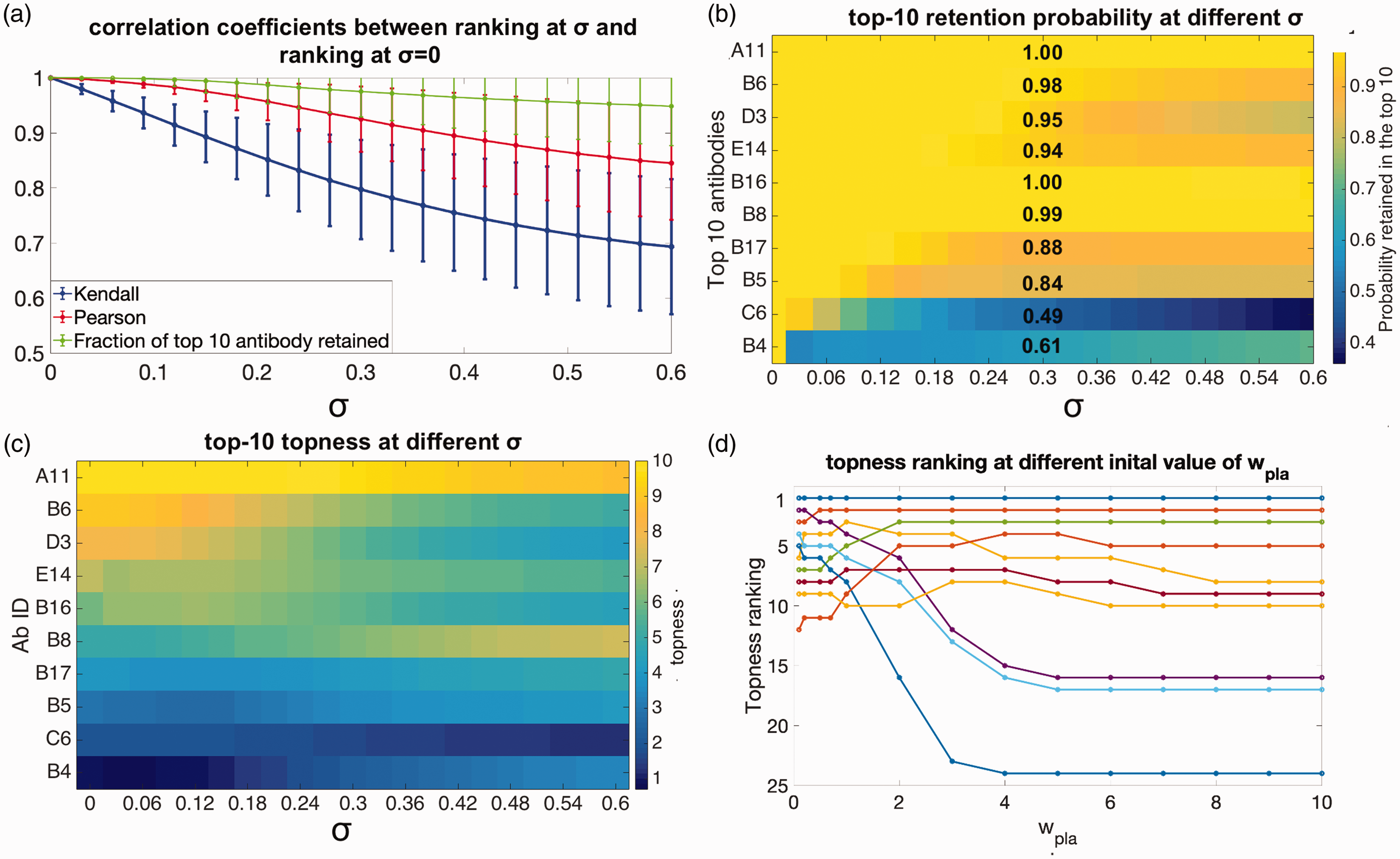
Robustness of the selected antibodies (a) mean values of the Pearson’s (red curve) and Kendall’s (blue curve) correlation coefficients, between the antibody rankings using our initial guesses for the weights, and for rankings obtained by randomizing the weights to degree σ. Green curve: Average fraction of the top 10 antibodies retained after randomizing the weights to degree σ. (b) The probability antibody candidates are retained in the top 10, as a function of the error in the weights σ, plotted according to the color scale on the right. The retention probabilities at $σ = \min (σ_{max}, 0.3)$ are explicitly given. (c) The topness (t₁₀) values for the antibodies in panel (b), plotted according to the right color bar scale as a function of increasing σ. (d) The topness ranking result for the antibodies as the initial weight w_pla is varied over a large range $0.1 < w_{pla} < 10$ .

A re-interpretation of Figure 6(a) is possible. We may consider the initial, σ = 0 values of the weights as the “true” weights that should be applied to the criteria, and σ as the error in our guesses for these true weights. Then the decrease in correlation coefficient, and related quantities such as how many of the top 10 candidates were retained given an error in our guess for the weights, may be studied as the error σ is increased. This gives a measure of the robustness of the predictions at a given stage of the screening.

In this light, we are likely to be significantly more interested in how robust are, say, the top 10 picks that were obtained using our initial guesses for the weights. We answer this question as follows: first we note the top 10 antibodies according to our initial guess for the screening criteria weights. Then we randomize weights as above, and count the fraction f of the original 10 that still remain in the new top 10 corresponding to the randomized weights. This fraction varies depending on the particular set of weights chosen, but has a well-defined average for a given value of σ. Again perhaps counter-intuitively, the average fraction $< f >$ at the uncertainty $σ = \min (σ_{max}, 0.5)$ is 0.95, meaning that on average, about 9 out of the top 10 picks remain in the top 10 when the weights are randomized to a significant degree. The average remaining fraction of top 10 picks $< f >$ vs. σ is shown as the green line in Figure 6(a).

In Figure 6(b), we quantify the probability each particular antibody in the top 10 is retained, as weights are randomized, i.e. the retention probability p₁₀ for the initial top 10 antibodies. The figure indicates the top 10 antibodies, ordered from 1st (A11, top) to 10th (B4, bottom), according the initial guesses for the weights ( ${w_{i}^{0}}$ and σ = 0; note that this ranking differs slightly from that in Supplemental Table S1, which gives the topness ranking from sampled weights having $σ = \min (σ_{max}, 0.5)$ ). For small standard deviation σ, antibodies are nearly always retained in the top 10, but as the error increases, antibodies near the bottom of the top 10 begin to occasionally drop out. The retention probability specifically at $σ = 0.3$ is listed in the figure. The antibodies C6 and B4 have the lowest retention probability at maximum σ: 36% and 70%, respectively. Some antibodies—A11, B16 and B8—are retained in the top 10 with probability greater than 95% over the whole range of σ. This reinforces their reliability as top picks, which would warrant (re)prioritizing them for further screening.

In Figure 6(c), we show the how the topness values change as the weight-uncertainty σ increases, for the initial top 10-ranked antibodies using the initial guesses $w_{i}^{0}$ . Again, it shows that the top 6 antibodies are very robust over the whole range of σ. We also see that B8 in particular shows increasing topness as σ is increased, again implying that that antibody should be re-prioritized.

We now consider what happens to the topness ranking as we vary the initial weight w_i of one screening criterion such as B_pla from say 0.1 to 10 ( $0.1 < w_{pla} < 10$ ). We note that this is a much larger range of weights than what would occur during the above randomization. This amounts to varying the importance of plaque binding, from essentially negligible importance to making it the dominant criterion. The results are shown in Figure 6(d). As w_pla is increased to 10, the top ranked candidates become those that performed best in the plaque binding assay. These candidates are not the same as the top ranked candidates when B_pla is neglected. For example, the 1st, 2nd, and 3rd-ranked candidates at the initial weight w_pla = 1 are A11, D3, E14, respectively, and their rankings change to 1, 2, and 8 when w_pla = 10, and 1, 3, and 6 when w_pla = 0.1. This again emphasizes the importance of user-based judgement in weighting the criteria appropriately from the outset to determine the potential of a given candidate.

We lastly note that there are other ways of organizing screening criteria, such as taking ratios rather than differences, e.g. $B_{o} / B_{m}$ rather than $B_{o} - B_{m}$ . Our results have used differences in screening criteria. A comparison of the ranking results using differences vs. using ratios is made in Supplemental Figure S6.

3.4 Sensitivity to the addition of new screening criteria

We can test what happens to the rankings when an additional screening criterion is added. A subset of 26 of the above 66 antibodies were subject to more time-intensive experimental screening, involving immunohistochemical measurements of plaque binding; see column 10 of Supplemental Table S1. This additional data may be used to rank this subset of antibodies among each other, and also compare their rankings before and after additional data is added. We describe this analysis further in the Supporting Information (see “Sensitivity to the addition of new screening criteria” in Supporting Information). The resulting rankings for eight screening criteria are given in Supplemental Table S1. Supplemental Figure S7 shows that, at least for the case of adding an 8th criterion with weight comparable to the other criteria, the trend in ranks does not qualitatively change.

Interestingly, if we used $d_{-}$ in equation (2) rather than d_c in equation (4), the correlation between the 7 D and 8 D rankings decreases from $(r, p) = (0.94, 1$ e- $12)$ to $(r, p) = (0.87, 5$ e- $9)$ . This observation implies that the closeness d_c used in the TOPSIS method, which uses two distances $d_{-}$ and $d_{+}$ , is a measure of ranking that is somewhat more robust to the addition of criteria than rankings obtained by simply using the distance $d_{-}$ from the origin.

3.5 Visualization of antibody rankings in screening space

We project the screening values of the 26 antibodies having data for eight screening tests, from the 8 D Hilbert space to a 3 D space, so that we may visualize them. To make this projection, we construct a 26 × 8 matrix containing all of the antibodies’ screening criteria. Then we perform a principal component analysis (PCA) on this matrix, and take the top three components, PC₁, PC₂, PC₃, as the x, y, z axes in what will be a 3 D projection of the higher-dimensional Hilbert space. The coordinates of each antibody are given by projecting the antibody’s 8 D radius onto the above three principal components. The 3 D projections for all 26 antibodies are shown in Figure 7(a). The first three principal components capture 61%, 15%, and 10% of the variance of the dataset, respectively (see supplemental Figure S8.)

Figure 7.

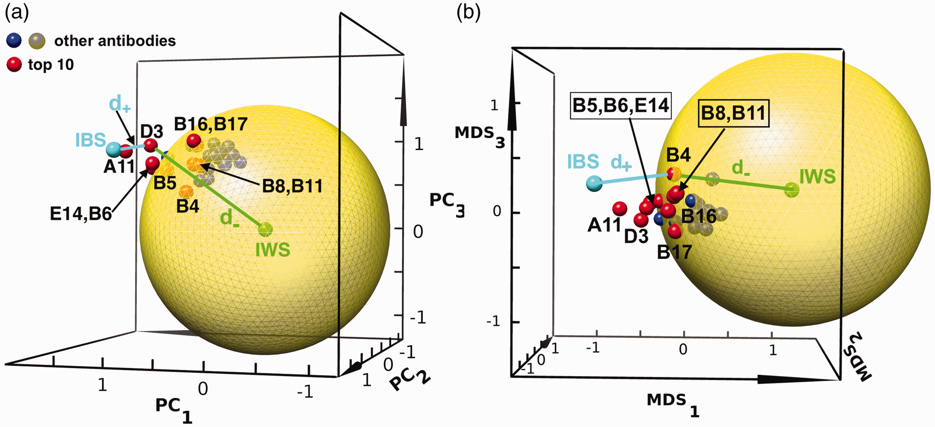
The projection of antibodies from 8 D to the first three principal components, PC₁, PC₂, and PC₃ and the first three MDS components, MDS₁, MDS₂, MDS₃ (see text). The top 10 antibodies are plotted in red spheres, with corresponding antibody labels from Supplemental Table S1. The remaining antibodies are shown as blue/grey spheres as indicated in the legend. The large, semi-transparent yellow solid sphere is the projection of the 8 D-spherical surface with radius set so that the top 10 ranking antibodies are outside of it in the higher-dimensional Hilbert space. The ideal best solution (IBS) and ideal worst solution (IWS) as defined in the TOPSIS method are labeled in cyan and green, respectively. The distances to the IWS and IBS are shown for a representative candidate (D3 in panel (a), B4 in panel (b)). (a) In the reduced-dimensionality 3 D PCA space, five of the top 10 antibodies (B4, B5, B8, B11 and B17) are projected inside the 3 D sphere; five others are outside of the 3 D-sphere projection. The IBS point is located at (1.2, 1.3, 0.8) and the IWS point is located at (0,0,0). (b) In the reduced-dimensionality 3 D MDS space, only one of the top 10 antibodies (B4) is projected inside the 3 D sphere, consistent with the fact that MDS projections better preserve higher-dimensional distances. The IBS point is located at (−0.8, −0.1, 0.2) and the IWS point is located at (1.1, 0.6, 0.2).

Purely for rendering the projected antibodies in Figure 7, we have taken the mean 8 D radius for each antibody upon randomization of the weights, using $σ_{i} = \min (w_{i} / \sqrt{3}, 0.5)$ . This may be thought of as a “most representative” sample of radii for the antibodies.

As shown and described in Figure 7(a), a sphere radius $r_{0}^{8 D}$ may be defined such that the top 10-ranked antibodies are just outside of it. Upon projection to 3 D, five of the top 10 ranking antibodies are actually inside the 3 D-projected sphere, since five orthogonal dimensions are lost in making the projection. Likewise, the projection of the 8 D surface into 3 D space is a solid sphere with the corresponding projected radius. All the antibodies with $r^{8 D} < r_{0}^{8 D}$ will be inside the corresponding 3 D sphere. To see these features intuitively, we note that the projection of the surface of a ball onto the table below it is a solid (filled) 2 D circular “shadow”. A point above the sphere in 3 D space but within the perimeter of its shadow would be projected to be inside the circular shadow in the 2 D projection. Likewise, all points within the 3 D sphere will be within the 2 D projection.

Because the PCA technique does not preserve the relative distance between two points in the reduced-dimensional space, we employ “Multidimensional Scaling” (MDS)⁵⁶ to render our 8 D data in 3 D space, while optimally preserving pairwise distances between candidates in the dataset. Using this metric, we can see that now nine of the top 10 antibodies are projected outside of the yellow solid sphere (Figure 7(b)). In Supplemental Figure S9, we perform the additional projection of the 8 D measurements onto a 2 D plane for both the PCA and MDS methods.

3.6 Testing robustness with a randomly generated dataset

We have repeated the above procedure of obtaining the rankings by various metrics on a synthetic correlated Gaussian dataset, constructed as described in section 2. Figure 8(a) gives the probability that each antibody is contained within the top 10 (top 10 retention probability), for weight uncertainty $σ_{i} = \min (w_{i} / \sqrt{3}, 0.5)$ . This may be compared with Figure 4(a); again, only antibodies with nonzero retention probability are shown. Figure 8(b) gives the retention probability to be in the top-n ranked candidates, as a function of n. Candidates are chosen as the top 10 ranked by topness t₁₀. Mean ranking is given after each antibody ID. The values in Figure 8(b) at n = 10 are equivalent to the values for the corresponding antibodies in Figure 8(a). Comparing Figure 8(b) with the analogous Figure 4(c), we observe much less dominance by any candidate or group of candidates in Figure 8(b), consistent with a lack of outliers, as expected from the Gaussian construction of this data set. Figure 8(c) shows scatter plots of the mean ranking and retention probability ranking p₁₀ vs. the ranking by topness t₁₀. While the top four antibodies correlate perfectly between metrics, lower-ranked antibodies show much more scatter (c.f. Figure 4(d)). Figure 8(d) shows the retention probability for each of the initial top 10 antibodies to remain in the top 10, now as a function of σ. For this data, it is useful to interpret the σ = 0 values as the “correct” values of the weights for each criteria, and the various values of the weights at $σ > 0$ as containing errors due to uncertainty. The retention probability specifically at $σ = 0.3$ is listed in the Figure 8(d).

Figure 8.

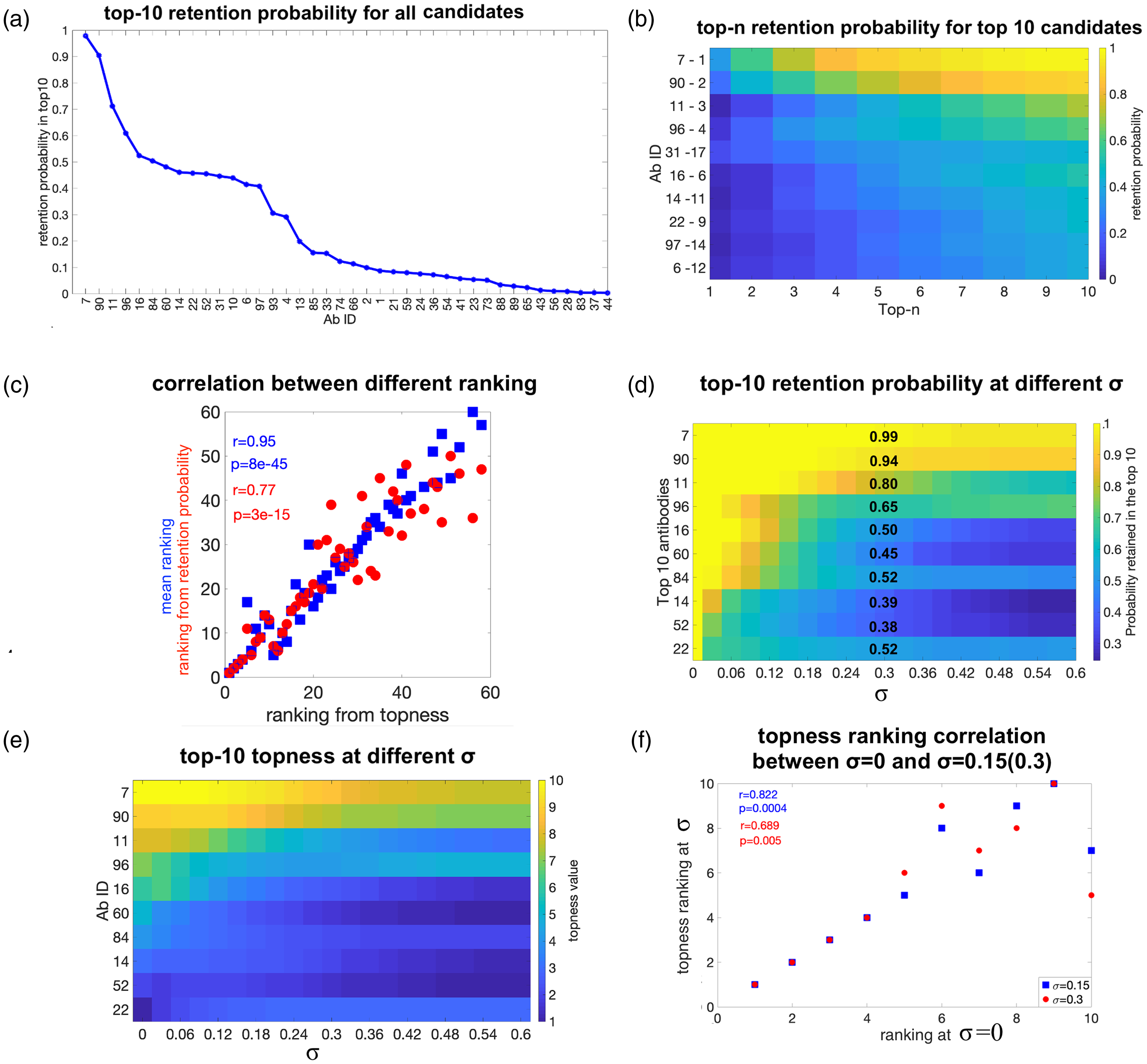
Validation tests of the method using different metrics, for synthetic data. (a) The top 10 retention probability with weights uncertainty $σ = \min (\frac{w}{\sqrt{3}}, 0.5)$ . (b) Retention probability for antibodies to be ranked within the top-n. Candidates are sorted by their topness score at $σ_{i} = \min (w_{i} / \sqrt{3}, 0.5)$ . The mean rank is listed after each candidates for comparison (c.f. Figure 4(c)). (c) The scatter plots of the mean and retention probability ranking vs. the topness ranking. (d) Same as Figure 6(b), but for the randomly generated dataset with correlation coefficients shown in Figure 1(b). Candidates in panels (d, e) are sorted by their topness at σ = 0. (E) Topness values for the top 10 ranked antibodies as a function of the error in weights σ. (f) Scatter plot of the antibody rankings for $σ = 0.15, 0.3$ vs. rankings at σ = 0.

Interestingly, the retention probabilities are distributed differently for correlated, Gaussian random data than for real data: At $σ = 0.3$ , only two candidates are retained with probability $> 80 %$ (Figure 8(d)), while for our real data in Figure 6(b), eight of the top 10 are retained with $> 80 %$ probability, and six of the top 10 are retained with $> 90 %$ probability. This again supports the notion that those antibodies in the real data set are statistical outliers that would warrant prioritization and further screening.

Figure 8(e) shows the topness t₁₀ for the top 10-ranked antibodies at σ = 0, as a function of the error σ in the “correct” weights. We can see that as σ increases, the topness value of each antibody generally decreases, since the retention probability in the top m ( $m \leq 10$ ) decreases (c.f. Figure 6(c)). It is possible for some antibodies to improve their topness and thus their rank as σ increases, however. For example, the ranking of Ab22 increases from 10th to 5th (with topness increasing from 1 to 4) when the error σ increases from 0 to 0.6.

Figure 8(f) shows a scatter plot of the rankings at two values of σ (0.15 and 0.3), vs. the ranking at σ = 0. This is another way to depict the inaccuracies in ranking due to uncertainty in the criteria weights. We note again that this Gaussianly generated dataset does not have strong outliers and so is less robust to weight uncertainty than the real dataset. As for the real data set above, antibody ranking by mean or topness for synthetic Gaussian data is nearly independent of the distribution used for the uncertainty in weights (Supplemental Figure S10), at least for quasi-Gaussian, uniform or log-normal distributions.

3.6.1 Validation tests using a randomly generated dataset

To further validate the ability of the method to identify “true positive” and “true negative” candidates, we manually changed the screening values of the criteria for four candidates from the above 100 in the synthetic Gaussian dataset, as follows. For candidate A1, we increased the values of 8 of the 10 screening criteria to the maximum observed values for each of those criteria. For candidate A2, we increased the values of 3 of A1’s 8 maximal screening criteria to the maximum observed values for each of those criteria. For candidate A100, we decreased the values of the same 8 of 10 screening criteria as above to the minimum observed values for each of those criteria. For candidate A99, we decreased the values of three of A100’s eight minimal screening criteria to the minimum observed values for each of those criteria (the same three criteria as for A2). In this case, the candidates A1 and A100 may be thought of as the true positive and true negative candidates, respectively, and A2 and A99 may be thought of as a “strong positive” and “strong negative,” respectively.

The SMAA-TOPSIS method ranks candidates A1 and A100 as 1st and 100th, respectively, validating the method when true positives and true negatives are present (see Supplemental Figure S11). Interestingly, the strong positive (A2) and negative (A99) candidates are ranked 2nd and 94th, respectively, by the SMAA-TOPSIS algorithm. The algorithm is asymmetric in its choice of top and bottom candidates. Encouragingly, the method is more robust for its choice of top candidates.

3.7 Further validation using antibody data from the literature

To test the SMAA-TOPSIS method on existing antibody data from the literature, we have applied it to two data sets obtained to quantify the “developability” of a given antibody therapy. Jain et al.⁵⁷ have analyzed the landscape defined by 12 biophysical properties (i.e. screening criteria) for 137 clinical-stage antibodies. For some criteria, lower values are better, and for these we multiply the values by a minus sign and rank highest to lowest as usual. The 12 screening criteria partition into five clusters. To assign a weight to each criterion, we assign weight one to each cluster, so if a cluster has N criteria, then the weight for each criterion in this cluster is $1 / N$ . Uncertainties in weights are again given by the formula $σ_{i} = \min (w_{i} / \sqrt{3}, 0.5)$ .

Figure 9(a) shows the retention probability to be in the top-n candidates, vs. n. The top 10-ranked candidates by topness are shown, sorted according to the SMAA-TOPSIS method. The retention probability ranking is also given after each candidate, which may be compared with Figure 9(b), which plots the retention probability to be in top 10 candidates. Antibodies are sorted on the x-axis of Figure 9(b) in order of decreasing retention probability. Figure 9(c) illustrates a 3 D projection of the 12-dimensional space, by multi-dimensional scaling (MDS). These antibodies show much more clustering than those in Figure 7. There appears to be one notable outlier, rilotumumab, which is ranked 136.

Figure 9.

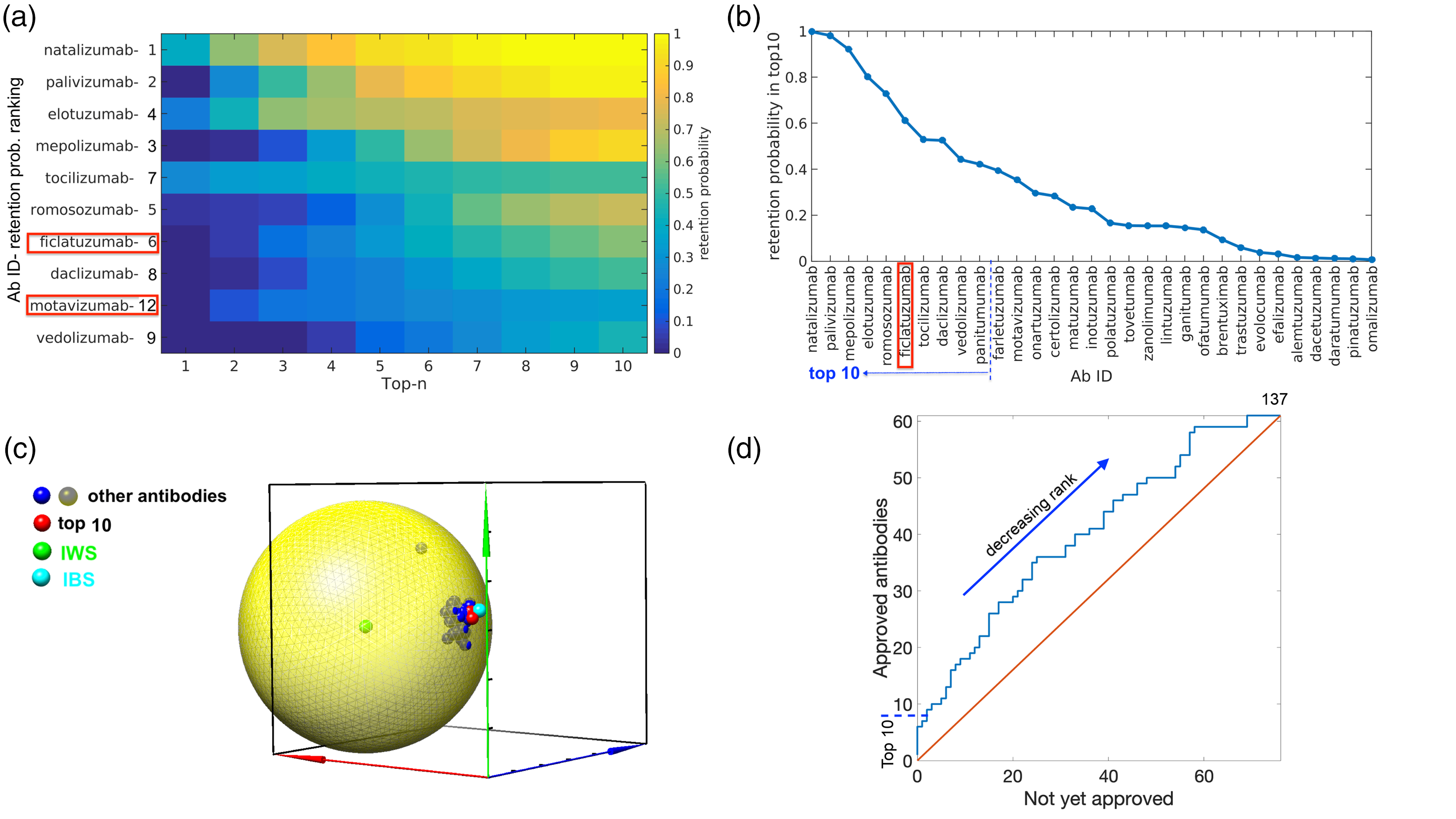
Validation results using antibodies that are either clinically approved or in development. (a) The retention probability to be within the top n-ranked candidates. Shown are the top 10 ranked antibodies of the cohort in Jain et al.,⁵⁷ as ranked by topness. Antibodies marked with red rectangles in panels (a, b) are those that are either not yet approved or discontinued, but still ranked in the top 10. (b) The retention probability to be in top 10 candidates. Antibodies are sorted on the x-axis in order of decreasing retention probability. (c) The 3-D MDS representation for the antibodies studied in Jain et al.⁵⁷ (d) An “ROC” plot, where approved antibodies are plotted against not-yet-approved antibodies. Antibodies are plotted from best ranked to worst ranked by SMAA-TOPSIS prediction, as the blue curve proceeds from lower left to upper right.

Figure 9(d) shows a variant of an “ROC” plot, wherein all 137 antibodies are plotted on the blue curve from best ranked (lower left) to worst ranked (upper right) by the SMAA-TOPSIS prediction using topness. If an antibody is approved, the blue curve takes a step upward, if an antibody is not yet approved, the curve takes a step to the right. This procedure constructs a type of receiver operating characteristic (ROC) curve, wherein approved antibodies are treated as true positives, and not-yet-approved antibodies are (tentatively) treated as false-positives, though they may be approved in the future. Discontinued antibodies in this list are also treated as false-positives. We emphasize this procedure is only intended to rank candidates on the physico-chemical screening characteristics; it is not a predictor of clinical success. We note, however, that 8 out of the top 10 candidates as ranked by topness have been approved, motavizumab is discontinued, and ficlatuzumab is in phase 2. Nine out of the top 10 candidates as ranked by retention probability have been approved, with ficlatuzumab in phase 2. Conversely, 8 of the bottom 10 topness-ranked candidates have not been approved yet (three are in phase 3 trials and five are in phase 2 trials).

As a second application of antibody data from the literature, Bailly et al.⁵⁸ have discussed the prediction of antibody “developability” profiles through early stage discovery screening. They studied nine physico-chemical properties (nine screening criteria) of 10 antibody variants, for which we follow their naming convention and label as mAb87 and mAb102-110. The nine screening criteria—which are quantities such as thermal stability, reduced aggregation propensity, and robustness against fragmentation or clipping—are classified into two groups, Priority 1 and Priority 2, depending on their importance for developability.⁵⁸ Here, we give the five criteria that were determined as Priority 1 a weight of 1 and uncertainty 0.5, while the four Priority 2 criteria are given weight 0.5 and uncertainty $0.5 / \sqrt{3}$ . Performing a SMAA-TOPSIS ranking with this dataset gives the results shown in Supplemental Figure S12, which appear to correlate well with the authors’ conclusions. First, mAb103 is ranked as having the best developability profile. On the other hand, a surprise from the present analysis is that mAb102 is ranked second best. This antibody had two non-optimal properties as determined by the authors, as opposed to mAb105, mAb106, and mAb107, which had only one non-optimal property. Other conclusions of the authors are also recapitulated in the SMAA-TOPSIS ranking, including (1) mutated IgG1 isotypes tend to be more developable than IgG4 isotypes (Figure S12B), (2) for IgG4 isotypes, the variable light chain ranking among variants studied is preserved (VL5 (mAb107) > VL7(mAb109) = VL8(mAb110) > VL6(mAb108) in the authors’ nomenclature⁵⁸), (3) several antibodies including the IgG4 mAb107 are significantly better than the parent IgG4 antibody mAb87. A plot of the retention probability, and a PCA plot projected in 3 D, are both shown in Supplemental Figure S12.

3.8 Further validation using other literature data

We conclude our results with a final validation of the method, by applying it to two additional data sets from the MCDM literature. Tsaur et al.⁵⁹ have used the TOPSIS method, but without any weight randomization, to rank three airlines. For screening values, they use triangular fuzzy numbers for 15 differently weighted criteria measuring service quality. Applying the SMAA-TOPSIS method developed here and using their derived weights as well as the mean performance values for each screening criterion, we directly reproduce their ranking (of airlines B, C, then A in their notation). However, because we allow for uncertainty in the weights, we can also find the probability that, for example, airline C is the top-ranked airline, and so on. Supplemental Figure S13 shows the probability that each airline is ranked first, second or third. This analysis can help quantify if one candidate performs either marginally or substantially better than another. For example Figure S13A,B shows that airline C ranks only marginally better than airline A, i.e. with some changes in the weights of the screening criteria, A would rank above C.

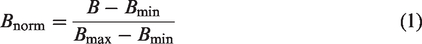
Opricovic et al. has compared the rankings obtained by two MCDM methods, TOPSIS and VIKOR—another method to obtain a compromise solution for a problem with conflicting criteria.²⁹ They rank three alternatives (mountains chosen by a beginner climber) based on two conflicting screening criteria (risk and altitude difference, with low risk and high altitude difference being desired). The two criteria are given equal weighting in their analysis. They illustrate an inconsistency with a particular formulation of TOPSIS when vector normalization of criteria is used, which is removed when using linear normalization.²⁹ We note that we have used linear normalization for our criteria in equation (1), which removes this problem. Applying the SMAA-Topsis method, we can see that even though we reproduce the ranking obtained by the authors originally (using either VIKOR or linearly normalized Topsis) of A2 >A1 $\approx$ A3, we see from Figure S13C that candidate A3 has a non-monotonic ranking probability distribution, and has a significantly higher probability than A1 to be the top candidate for some weights. A3, while ranking similarly to A1, thus appears as a “high risk-high reward” candidate. Ranking distributions can give additional insights to help choose between two comparable candidates.

4 Discussion

The main point of this analysis is to provide a method to maximize the confidence in a set of rankings, given the fact that the screening values and criteria weights are uncertain. We have introduced several new quantities here to determine the robustness of a given candidate’s rank, when either measurement error or weight/importance error are accounted for. These include the Topness and the Retention Probability. These quantities may be very useful when applied more broadly in other contexts involving multi-criteria decision making (MCDM).

There are several other methods that may be used to rank candidates in the MCDM problem,²⁷ including the so-called Fuzzy-TOPSIS method, which implements Fuzzy numbers to characterize screening criteria and weights.^41,42,60 Fuzzy numbers are especially suitable when no quantitative data is provided other than the relative importance of screening criteria or weights by linguistic variables (e.g. “very low”, “low”, “moderate”, “high”, and “very high”). It is an interesting topic of future research to systematically compare the results of the SMAA-TOPSIS method applied here with the Fuzzy-TOPSIS method (as well as other methods in MDCM). In preliminary analysis, we have found very similar results between the two methods: nine of the top 10 candidates ranked by SMAA-Topness remain in the top 10 when Fuzzy-TOPSIS is applied to our data, and the only candidate that fell out of the top 10 was ranked 9th by SMAA-TOPSIS, and 11th in Fuzzy-TOPSIS. There is no distinct advantage of Fuzzy-TOPSIS over SMAA-TOPSIS as a ranking method. In some aspects, regarding the uncertainty in criteria or weights, SMAA-TOPSIS allows a more detailed investigation.

Naturally, one cannot definitively rule out a candidate or guarantee a candidate’s success as further data becomes available. However, one utility of the method discussed here is to narrow down the cohort of candidates to a smaller subset that may be subsequently screened with more time-intensive or more rigorous tests.

We note that antibody B6, which over seven screening criteria was ranked second among the 66 candidates, and ranked first among 17 candidates to its specific epitope, has undergone further preclinical development.⁴⁹ Several other antibodies to this epitope (in the B-series of Table S1) ranked in the top 10. However, other top-ranked candidates, such as A11, may also be promising as effective therapeutics.

We have validated the method of ranking and identifying top candidates in several ways. Using synthetic data, the method could properly identify a priori constructed true positives and true negatives. We also constructed an ROC curve for approved antibodies vs. those still in clinical trials, which showed that the method preferentially identified approved antibodies as top candidates, and antibodies still under development as bottom candidates. When the method was applied to either clinical antibodies, or other cases from the general MCDM literature, it provided consistent conclusions as well as additional insights.

We have created a webserver (http://bjork.phas.ubc.ca) where the method may be applied to the user’s own data. Data are uploaded to the server in the form of a spreadsheet containing screening data for various candidates and criteria, as well as weight values to be applied to those criteria. Errors/uncertainty for the measurements and the weights can be input as well. The output includes the following: Rank-ordered lists of leading candidates according to both topness and mean ranking; histogram data and figures for the ranking distributions similar to Figure 3; a 3 D principal-component sphere and a 3 D MDS sphere similar to Figure 7; the probability data of each antibody to be at various ranks; the ranks with zero weight uncertainty (σ = 0); and the python scripts of the dimensionally reduced closeness (c.f. Figure 7) that may be opened from the program Chimera⁶¹ to facilitate visualization (see Supporting Information).

5 Conclusion

In this paper, we have applied a method from multi-criteria decision making (MDCM) known as Stochastic Multi-criteria Acceptability Analysis (SMAA2³⁴) to the problem of antibody drug candidate selection. To measure the quality of each candidate and thus rank them across several different screening criteria simultaneously, we used the Technique for Order Performance by Similarity to Ideal Solution (TOPSIS^27,28).

The retention probability and topness were defined to rank the best performing antibodies for their selection as candidate leads. The method here accounts for uncertainty in measurement values, as well as uncertainty in the user-defined weights of importance that are ascribed to the various performance screens. As a visual aid, the performance of the candidates may be rendered in the space of screening criteria by principal component analysis (PCA) or multidimensional scaling (MDS). For the real dataset of experimental screening measurements, the top-ranked candidates were observed to be statistical outliers, and including them in the cadre of leads was insensitive to the precise values of criteria weights.

As long as the importance of screening criteria are reasonably estimated, the ranking method provided here can broaden, refine, or change the scope of lead candidates selected from a large cohort. Choosing the best lead candidates for further development is not always an obvious task, especially when multiple screening criteria are performed, each of which may address different efficacy, ADME, or toxicity criteria. In practice, it is not always the same antibody or molecule that emerges as the clear winner across different tests. In these cases, incorporating algorithmic ranking methods into the researcher’s arsenal can provide a valuable tool in choosing lead candidates.

While preclinical screening cannot guarantee the success of a new drug, the method contained herein could help to increase the chances of success in downstream clinical trials, based on the user’s own screening criteria and estimates for their importance.

Particularly when the number of screening variables becomes large (e.g. of order 10 or more), and the weight that should be given to each is uncertain, the systematic solution to a task such as optimizing the selection of most-likely leads is a problem that—now and likely even more so in the future—will be best handled by computer algorithm, which should subsume and often correct the solutions obtained by intuitive guess.

Supplemental Material

sj-zip-1-smm-10.1177_09622802211002861 - Supplemental material for A method for systematically ranking therapeutic drug candidates using multiple uncertain screening criteria

Supplemental material, sj-zip-1-smm-10.1177_09622802211002861 for A method for systematically ranking therapeutic drug candidates using multiple uncertain screening criteria by Xubiao Peng, Ebrima Gibbs, Judith M Silverman, Neil R Cashman and Steven S Plotkin in Statistical Methods in Medical Research

Supplemental Material

sj-pdf-2-smm-10.1177_09622802211002861 - Supplemental material for A method for systematically ranking therapeutic drug candidates using multiple uncertain screening criteria

Supplemental material, sj-pdf-2-smm-10.1177_09622802211002861 for A method for systematically ranking therapeutic drug candidates using multiple uncertain screening criteria by Xubiao Peng, Ebrima Gibbs, Judith M Silverman, Neil R Cashman and Steven S Plotkin in Statistical Methods in Medical Research

Supplemental Material

sj-xlsx-3-smm-10.1177_09622802211002861 - Supplemental material for A method for systematically ranking therapeutic drug candidates using multiple uncertain screening criteria

Supplemental material, sj-xlsx-3-smm-10.1177_09622802211002861 for A method for systematically ranking therapeutic drug candidates using multiple uncertain screening criteria by Xubiao Peng, Ebrima Gibbs, Judith M Silverman, Neil R Cashman and Steven S Plotkin in Statistical Methods in Medical Research

Footnotes

Authors' Note

Xubiao Peng is now affiliated with Center for Quantum Technology Research, School of Physics, Beijing Institute of Technology, Beijing, China. Judith M Silverman Bill & Melinda Gates Medical Research Institute, 750 Republican St, Suite F309, Seattle, WA 98109, USA.

Acknowledgements

We acknowledge WestGrid (www.westgrid.ca) and Compute Canada/Calcul Canada () for providing computing resources.

Declaration of conflicting interests

The author(s) declared the following potential conflicts of interest with respect to the research, authorship, and/or publication of this article: SSP was the Chief Physics Officer of ProMIS Neurosciences until October 2020. NRC is the Chief Scientific Officer of ProMIS Neurosciences. XP has received consultation compensation from ProMIS. SSP, NRC, and XP are inventors on several pending patent applications directed to therapeutics for Alzheimer’s disease and which describe immunogens, antibodies and methods of their making as well as their use.

Funding

The author(s) disclosed receipt of the following financial support for the research, authorship, and/or publication of this article: This work was supported by Canadian Institutes of Health Research Transitional Operating Grant 2682, and the Alberta Prion Research Institute, Research Team Program Grant PTM13007.

ORCID iD

Steven S Plotkin

Supplemental material

Supplemental material for this article is available online.

References

Hughes

Rees

Kalindjian

, et al. Principles of early drug discovery. Br J Pharmacol 2011; 162: 1239–1249.

Taylor

The pharmaceutical industry and the future of drug development. Pharmaceut Environ 2015; 41: 1.

Holbein

MB.

Understanding FDA regulatory requirements for investigational new drug applications for sponsor-investigators.

J Investigative Med 2009; 57: 688–694.

Pritchard

Jurima-Romet

Reimer

, et al. Making better drugs: decision gates in non-clinical drug development. Nat Rev Drug Discov 2003; 2: 542.

Ylera

Harth

Waldherr

, et al. Off-rate screening for selection of high-affinity anti-drug antibodies. Analytical Biochem 2013; 441: 208–213.

Adam

Meng

Rizzo

, et al. Use of high-throughput mass spectrometry to reduce false positives in protease uHTS screens. J Biomol Screen 2015; 20: 212–222.

Birmingham

Selfors

Forster

, et al. Statistical methods for analysis of high-throughput RNA interference screens. Nat Meth 2009; 6: 569–575.

Gunter

Brideau

Pikounis

, et al. Statistical and graphical methods for quality control determination of high-throughput screening data. J Biomol Screen 2003; 8: 624–633.

Brideau

Gunter

Pikounis

, et al. Improved statistical methods for hit selection in high-throughput screening. J Biomol Screen 2003; 8: 634–647.

10.

Coma

Herranz

Martin

Statistics and decision making in high-throughput screening. In: Janzen

Bernasconi

(eds) High throughput screening: methods and protocols. 2nd ed. Berlin, Germany: Springer, 2009, pp.69–106.

11.

Nicolaou

Brown

Pattichis

CS.

Molecular optimization using computational multi-objective methods. Curr Opin Drug Discov

Develop 2007; 10: 316.

12.

Segall

MD.

Multi-parameter optimization: identifying high quality compounds with a balance of properties. Curr Pharmaceut Des 2012; 18: 1292.

13.

Nicolaou

Brown

Multi-objective optimization methods in drug design.

Drug Discov Today: Technol 2013; 10: e427–e435.

14.

Segall

Yusof

Champness

EJ.

Avoiding missed opportunities by analyzing the sensitivity of our decisions.

J Med Chem 2016; 59: 4267–4277.

15.

Sánchez-Rodríguez

Pérez-Castillo

Schürer

, et al. From flamingo dance to (desirable) drug discovery: a nature-inspired approach. Drug Discov Today 2017; 22: 1489--1502.

16.

Belton

Stewart

Multiple criteria decision analysis: an integrated approach. Berlin, Germany: Springer Science & Business Media, 2002.

17.

Mardani

Jusoh

MD Nor , et al. Multiple criteria decision-making techniques and their applications–a review of the literature from 2000 to 2014. Economic Res-Ekonomska Istraživanja 2015; 28: 516–571.

18.

Zopounidis

Doumpos

Multiple criteria decision making: applications in management and engineering. Heidelberg: Springer, 2017.

19.

Ananda

Herath

A critical review of multi-criteria decision making methods with special reference to forest management and planning. Ecol Econ 2009; 68: 2535–2548.

20.

Sadeghzadeh

Salehi

MB.

Mathematical analysis of fuel cell strategic technologies development solutions in the automotive industry by the TOPSIS multi-criteria decision making method. Int J Hydrogen Energy 2011; 36: 13272–13280.

21.

Steuer

Multiple criteria decision making combined with finance: a categorized bibliographic study. Eur J Operation Res 2003; 150: 496–515.

22.

Zavadskas

Turskis

Multiple criteria decision making (MCDM) methods in economics: an overview.

Technol Econ Develop Econ 2011; 17: 397–427.

23.

Pohekar

Ramachandran

Application of multi-criteria decision making to sustainable energy planning-a review. Renew Sustain Energy Rev 2004; 8: 365–381.

24.

Huang

Keisler

Linkov

Multi-criteria decision analysis in environmental sciences: ten years of applications and trends.

Sci Total Environ 2011; 409: 3578–3594.

25.

Memariani

Amini

Alinezhad

Sensitivity analysis of simple additive weighting method (SAW): the results of change in the weight of one attribute on the final ranking of alternatives. J Optimiz Industrial Eng 2009; 4: 13–18.

26.

Saaty

TL.

Decision making with the analytic hierarchy process. Int J Services Sci 2008; 1: 83–98.

27.

Hwang

Yoon

Multiple attribute decision making: Methods and applications a state-of-the-art survey, vol. 186. Berlin, Germany: Springer Science & Business Media, 2012.

28.

Yoon

Hwang

CL.

Multiple attribute decision making: an introduction, vol. 104. Thousand Oaks, CA: Sage Publications, 1995.

29.

Opricovic

Tzeng

GH.

Compromise solution by MCDM methods: a comparative analysis of VIKOR and TOPSIS. Eur J Operation Res 2004; 156: 445–455.

30.

Brans

Mareschal

PROMETHEE methods. In: Multiple criteria decision analysis: state of the art surveys. Heidelberg: Springer, 2005, pp.163–186.

31.

Polatidis

Haralambopoulos

Munda

, et al. Selecting an appropriate multi-criteria decision analysis technique for renewable energy planning. Energy Sources, Part B 2006; 1: 181–193.

32.

Figueira

Mousseau

Roy

ELECTRE methods. In: Multiple criteria decision analysis: state of the art surveys. Heidelberg: Springer, 2005, pp.133–153.

33.

Greco

Ehrgott

Figueira

JR.

Trends in multiple criteria decision analysis, volume 142. Heidelberg: Springer Science & Business Media, 2010.

34.

Lahdelma

Salminen

SMAA-2: Stochastic multicriteria acceptability analysis for group decision making. Operation Res 2001; 49: 444–454.

35.

Hokkanen

Lahdelma

Miettinen

, et al. Determining the implementation order of a general plan by using a multicriteria method. J Multi-Criteria Decis Analys 1998; 7: 273–284.

36.

Tervonen

Figueira

Lahdelma

, et al. A stochastic method for robustness analysis in sorting problems. Eur J Operation Res 2009; 192: 236–242.

37.

Okul

Gencer

Aydogan

EK.

A method based on SMAA-topsis for stochastic multi-criteria decision making and a real-world application. Int J Inform Technol Decis Making 2014; 13: 957–978.

38.

Chang

DY.

Applications of the extent analysis method on fuzzy AHP. Eur J Operation Res 1996; 95: 649–655.

39.

Chu

TC.

Facility location selection using fuzzy TOPSIS under group decisions.

Int J Uncertainty, Fuzziness Knowledge-based Syst 2002; 10: 687–701.

40.

Nădăban

Dzitac

Fuzzy TOPSIS: A General View. Proc Comput Sci 2016; 91: 823–831.

41.

Yang

Hung

CC.

Multiple-attribute decision making methods for plant layout design problem.

Robotics Comput-Integr Manuf 2007; 23: 126–137.

42.

Chen

CT.

Extensions of the TOPSIS for group decision-making under fuzzy environment.

Fuzzy Sets Syst 2000; 114: 1–9.

43.

Xiong

A extended TOPSIS method for the stochastic multi-criteria decision making problem through interval estimation. In: Second international workshop on intelligent systems and applications (ISA), 2010, IEEE, pp.1–4.

44.

Yoon

A reconciliation among discrete compromise solutions. J Operation Res Soc 1987; 38: 277–286.

45.

Plotkin

Systems and methods for predicting misfolded protein epitopes by collective coordinate biasing. Patent WO2017079836, https://patentscope.wipo.int/search/en/detail.jsf?docId=WO2017079836&redirectedID=true, 2016.

46.

Peng

Cashman

Plotkin

SS.

Prediction of misfolding-specific epitopes in SOD1 using collective coordinates.

J Phys Chem B 2018; 122: 11662–11676.

47.

Cleary

Walsh

Hofmeister

, et al. Natural oligomers of the amyloid-β protein specifically disrupt cognitive function. Nat Neurosci 2005; 8: 79.

48.

Cline

Bicca

Viola

, et al. The amyloid-β oligomer hypothesis: beginning of the third decade. J Alzheimer’s Dis 2018; 64: S567–S610.

49.

Gibbs

Silverman

Zhao

, et al. A rationally designed humanized antibody selective for amyloid beta oligomers in Alzheimer’s disease. Scientific Rep 2019; 9: 9870.

50.

McAlary

Plotkin

Cashman

NR.

Emerging developments in targeting proteotoxicity in neurodegenerative diseases.

CNS Drugs 2019; 33: 883–904.

51.

Plotkin

Cashman

NR.

Passive immunotherapies targeting Aβ and tau in Alzheimer’s disease.

Neurobiol Dis 2020; 144: 105010.

52.

Plotkin

Cashman

N-terminal epitopes in Amyloid beta and conformationally-selective antibodies thereto. Patent WO2017079831, https://patentscope.wipo.int/search/en/detail.jsf?docId=WO2017079831&redirectedID=true (2016).

53.

Silverman

Gibbs

Peng

, et al. A rational structured epitope defines a distinct subclass of toxic amyloid-beta oligomers. ACS Chem Neurosci 2018; 9: 1591–1606.

54.

Arthur

Vassilvitskii

k-means++: The advantages of careful seeding. In: Proceedings of the eighteenth annual ACM-SIAM symposium on discrete algorithms, Society for Industrial and Applied Mathematics, Philadelphia, 2007, pp.1027–1035.

55.

Daniel

WW.

Applied nonparametric statistics. Boston, MA: PWS-kent, 1990.

56.

Cox

MA.

Multidimensional scaling. Boca Raton, FL: CRC Press, 2000.

57.

Jain

Sun

Durand

, et al. Biophysical properties of the clinical-stage antibody landscape. Proc Natl Acad Sci 2017; 114: 944–949.

58.

Bailly

Mieczkowski

Juan

, et al. Predicting antibody developability profiles through early stage discovery screening. Mabs 2020; 12: e1743053.

59.

Tsaur

Chang

Yen

The evaluation of airline service quality by fuzzy mcdm. Tourism Manage 2002; 23: 107–115.

60.

Yuen

KKF.

Combining compound linguistic ordinal scale and cognitive pairwise comparison in the rectified fuzzy TOPSIS method for group decision making.

Fuzzy Optimiz Decis Making 2014; 13: 105–130.

61.

Pettersen

Goddard

Huang

, et al. UCSF Chimera-a visualization system for exploratory research and analysis. J Computat Chem 2004; 25: 1605–1612.

Supplementary Material

Please find the following supplemental material available below.

For Open Access articles published under a Creative Commons License, all supplemental material carries the same license as the article it is associated with.

For non-Open Access articles published, all supplemental material carries a non-exclusive license, and permission requests for re-use of supplemental material or any part of supplemental material shall be sent directly to the copyright owner as specified in the copyright notice associated with the article.

0.01 MB

0.00 MB

4.43 MB

0.04 MB