
Abstract
Dose–response models express the effect of different dose or exposure levels on a specific outcome. In meta-analysis, where aggregated-level data is available, dose–response evidence is synthesized using either one-stage or two-stage models in a frequentist setting. We propose a hierarchical dose–response model implemented in a Bayesian framework. We develop our model assuming normal or binomial likelihood and accounting for exposures grouped in clusters. To allow maximum flexibility, the dose–response association is modelled using restricted cubic splines. We implement these models in R using JAGS and we compare our approach to the one-stage dose–response meta-analysis model in a simulation study. We found that the Bayesian dose–response model with binomial likelihood has lower bias than the Bayesian model with normal likelihood and the frequentist one-stage model when studies have small sample size. When the true underlying shape is log–log or half-sigmoid, the performance of all models depends on choosing an appropriate location for the knots. In all other examined situations, all models perform very well and give practically identical results. We also re-analyze the data from 60 randomized controlled trials (15,984 participants) examining the efficacy (response) of various doses of serotonin-specific reuptake inhibitor (SSRI) antidepressant drugs. All models suggest that the dose–response curve increases between zero dose and 30–40 mg of fluoxetine-equivalent dose, and thereafter shows small decline. We draw the same conclusion when we take into account the fact that five different antidepressants have been studied in the included trials. We show that implementation of the hierarchical model in Bayesian framework has similar performance to, but overcomes some of the limitations of the frequentist approach and offers maximum flexibility to accommodate features of the data.
1 Introduction
Dose-response associations examine the effect of different levels of exposure (e.g. levels of smoking or drug doses) on a health outcome.1,2 In pairwise meta-analysis,3–5 combining dose–response associations from different studies and settings may lead to more precise and generalizable conclusions. 6 When aggregate-level data are available from multiple studies, dose–response associations can be synthesized using either a one-stage or two-stage model. The one-stage model is implemented as a linear mixed model, which estimates a dose–response fixed effect and accounts for the heterogeneity by allowing shapes to vary across studies. 7 In a two-stage model, the dose–response model is fitted first within each study, and then the regression coefficients (or shape characteristics) are synthesized across studies.8–10
The one-stage model takes into account heterogeneity but provides relevant information via the estimate of a between-studies variance–covariance matrix. The two-stage model employs standard meta-analytical techniques and provides the usual heterogeneity measures, such as I2, in case this is of interest. However, to fit non-linear shapes, frequentist implementation of the two-stage model requires multiple dose levels to be reported in each study. For example, if the dose–response curve is assumed to be approximated by a
The one-stage and two-stage models are implemented in a frequentist setting, and their performance has been evaluated in simulations and examples. 11 Fitting dose–response meta-analysis in a Bayesian framework, in the form of a hierarchical model, is, in our view, highly desirable. Several papers12,13 have described the advantages of Bayesian evidence synthesis. First, Bayesian models14,15 can be easily extended to incorporate, for example, study-specific covariates, to combine observational and randomized data, or to deal with multiple outcomes and exposure types. Second, one can employ informative priors for the dose–response shape to reflect expert knowledge or evidence from external data sources. Third, one can easily extend the model to explore the variation in dose–response curves within and across groups of similar exposures or drugs. Finally, probabilistic statements follow naturally as the posterior distributions can be interpreted as the true distributions of quantities of interest as uncertainty about all parameters is incorporated in the results.16,17
The paper is structured as follow. In Section 2 we present a Bayesian hierarchical dose–response meta-analysis model with normal or binomial likelihood and the cluster-specific dose–response model. The evaluation of the properties of the models follows in Section 3, alongside comparisons with the frequentist model in a simulations study. In Section 4, we re-analyze a dataset of the dose–response association of various doses of antidepressants. Finally, we discuss the strengths and limitations of the model in Section 5.
2 Methods
We introduce a Bayesian hierarchical model for dose–response meta-analysis. We focus on a dichotomous outcome, although the models could easily accommodate continuous outcomes.
2.1 Notation
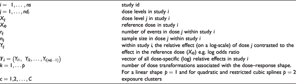
Table 1 summarizes the notation. Suppose there are
Notation in aggregated-level data in dose–response meta-analysis.
2.2 Dose–response meta-analysis model
We propose a hierarchical two-level model. In the first level, the dose–response model is fitted within each study assuming either normal (normal dose–response model) or binomial likelihood (binomial dose–response model) for the observed data. In the second level, we synthesize the dose–response regression coefficients across studies. The hierarchical structure allows coefficients to borrow strength across studies, via the exchangeability assumption.
2.2.1 Dose–response model within each study.
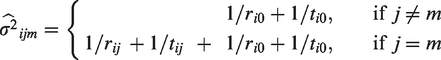
Within each study 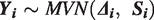
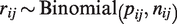
If the data are from a randomized trial and the table of counts is available, it is straightforward to assume a binomial distribution of events

Note that continuous outcome data can be accommodated if
2.2.2 Dose–response functions.
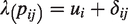
The underlying relative effect 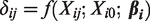

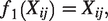
and
The total number and location of knots should be identical for all studies, when
2.2.3 Synthesize dose–response functions across studies.
In dose–response meta-analysis, the study-specific regression coefficients 
This model acknowledges the presence of a distribution of true dose–response relationships underlying the studies and is capable of predicting study-specific curves by borrowing strength from their variation across studies.
Note that for studies with
2.3 Dose–response meta-analysis model accounting for clustering in the exposure
Consider an exposure (or drug) variable that can take on different values. For example, daily intake of omega 3 fatty acids in relation to risk of cardiovascular events, possibly accounting for the different assessment of omega 3 (food supplements versus diet with fish and nuts). The differences between these two dose–response curves can be modelled by inserting type-specific regression coefficients
Overall, for a random of exposure clusters 
Next, 
At the next step, the cluster-specific dose–response associations 
2.4 Predicting an absolute mean response to a dose
Once the data are synthesized and the dose–response parameters are estimated, we can predict the absolute mean response for any dose within the range of studied dose levels. These predictions are straightforward within a Bayesian model as the total uncertainty in the parameters is propagated in the final predictions. Assume there is a natural reference dose, such as a dose zero or no-exposure (baseline dose). The observations
Then, the estimated common baseline mean effect 
2.5 Bayesian estimation
We will use Markov chain Monte Carlo (MCMC) techniques to estimate all parameters in a Bayesian setting. An approximate non-informative prior distribution is chosen for the coefficients and the baseline effects 
Given that both in the simulations and in the example our outcome is dichotomous and measured on the natural log scale, we place a half-normal prior to the heterogeneity parameter

This heterogeneity prior is minimally informative in most cases as ORs rarely exceed 5 and hence the underlying values of
For correlations 
All Bayesian models are implemented in JAGS within R.26,27 The codes can be found in GitHub at https://github.com/htx-r/DoseResponsePMA. To obtain the spline transformations, we use the rcs function from the rms package. 28 To evaluate the convergence of the models, we employed various diagnostic tools for MCMC included in the coda package. 29 We explored convergence plots for the MCMC (histograms, trace plots, Geweke plot and Gelman-Rubin plot) and relevant statistics (Raftery and Lewis statistic and Heidelberger and Welch test). 30
3 Simulations study
We aim to investigate the agreement between the estimations of the dose–response meta-analysis curve under our two Bayesian models, assuming random-effects for the coefficients, and the frequentist one-stage model. 31 The codes are available in GitHub.
3.1 Simulation design
We investigated the performance of the three models assuming that the true dose–response function is curvilinear (setting 1), half-sigmoid or log–log (setting 2). Characteristics of the simulated settings are summarized in Table 2.
Description of simulation settings.
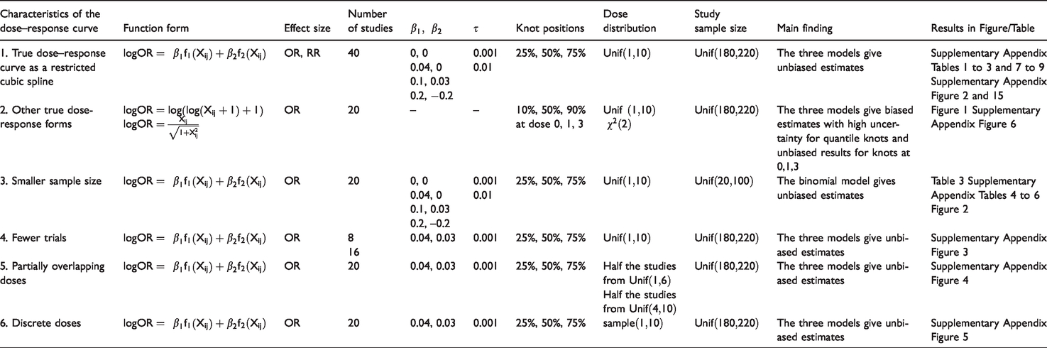
Under the assumption of a curvilinear relationship (setting 1), we used restricted cubic splines with three knots at fixed percentiles (25th, 50th, and 75th) of the dose, with shape defined by the spline coefficients. We modelled the logOR and the logRR. For 40 clinical trials, we simulated study-level aggregated data. For each study, we simulated two non-zero doses from uniform distribution
Using
Following the same steps as in logOR above, we simulated the dataset expressing the underlying treatment effect, instead, in terms of risk ratio
In the second setting (Table 2), we assumed the true shape is log–log (
The other four settings in Table 2 result from modifying setting 1. First, we assumed smaller trials by generating the sample size per dose as
The Bayesian models were estimated using 1×
For each method, we estimated the mean bias in the regression coefficients
3.2 Simulation results
3.2.1 Setting 1.
Supplementary Appendix Tables 1 to 3 present the results from the eight scenarios of the first setting for logORs using splines. Supplementary Appendix Figure 2 shows the average estimated curves for scenarios 2 to 4 (results from scenarios 6 to 8 provide similar conclusions to those in supplementary Appendix Figure 2; scenarios 1 and 5 refer to no dose–response association and are not presented in the figure). The three estimated dose–response lines are indistinguishable and all three models perform very well (supplementary Appendix Tables 1 to 3). The binomial Bayesian model has a slightly lower bias in the coefficients than the normal Bayesian and the frequentist approach in all scenarios. The spline coefficients
3.2.2 Setting 2.
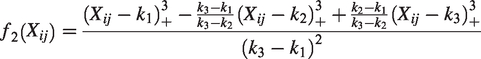
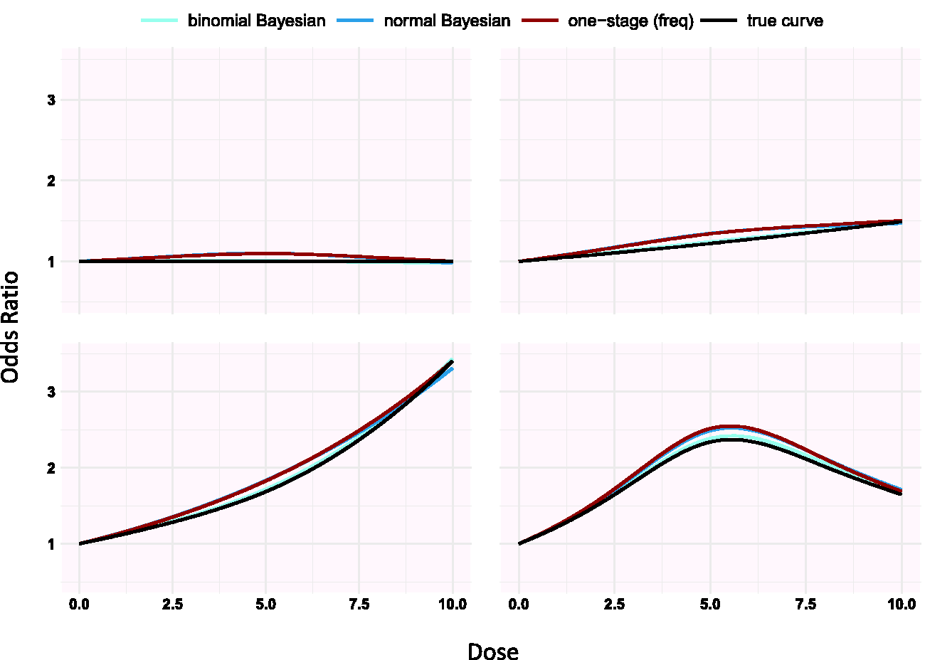
Simulating under different shapes, we found that estimations from the three models improves when knots are placed in dose ranges where the risk changes a lot compared to when we set knots at 10%, 50% and 90% percentiles as suggested by Harrell 24 (see Figure 1 and supplementary Appendix Figure 6).
3.2.3 Setting 3.
Modifications of setting 1 resulted in similar very good performance of all three models, with one exception. We found that the binomial Bayesian model gives less biased dose–response curve estimates compared with the normal Bayesian and frequentist models (see Table 3, Figure 1, and supplementary Appendix Tables 4 to 6).
Simulations scenarios in setting 3 in Table 2 for a spline dose–response association assuming random effects for
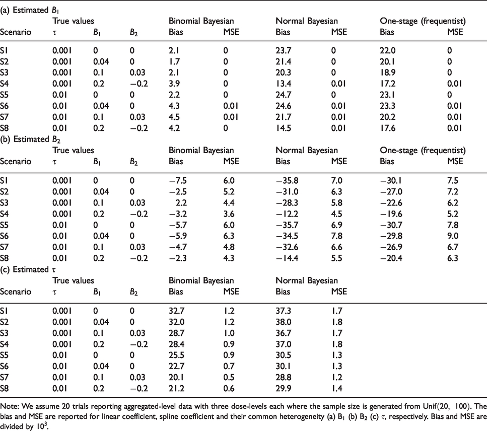
Note: We assume 20 trials reporting aggregated-level data with three dose-levels each where the sample size is generated from
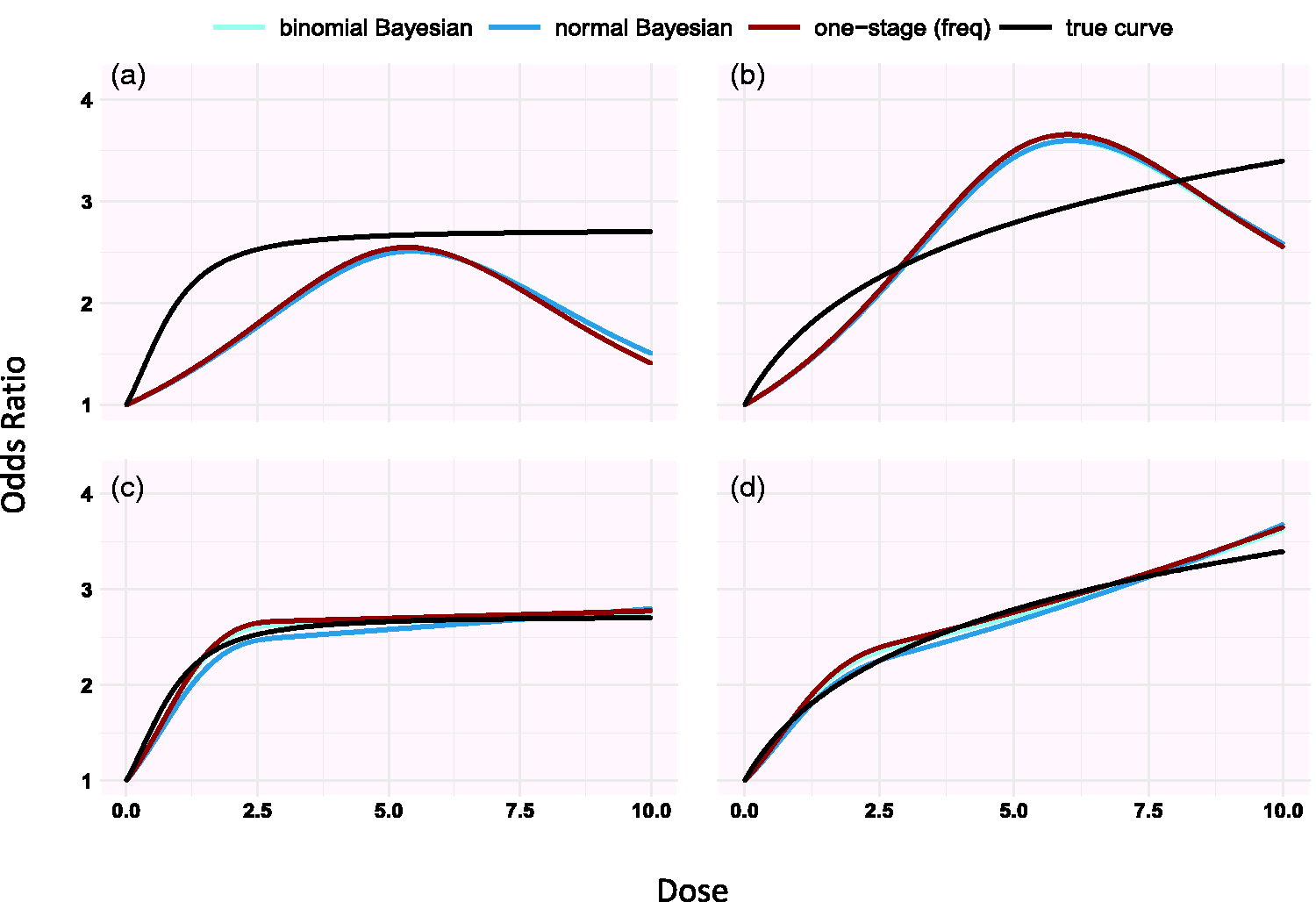
Simulation results for the half-sigmoid model (panels a, c) and the log-log dose model (panels b, d) estimated using restricted cubic splines (setting 2 in Table 2). Knots are placed in 10%, 50% and 90% quantiles in panels a and b and at doses 0, 1, 3 in panels c and d. The doses are generated from Unif(0, 10).
Overall, the spline coefficients
Additional results from setting 3 are presented in supplementary Appendix Tables 4 to 6. The coverage of all estimates exceeds 87%; coverage with the binomial Bayesian model is slightly larger than with the normal likelihood models. The power to detect a nonzero linear coefficient
3.2.4 Settings 4–6.
In settings 4, 5 and 6, the three estimated dose–response curves are indistinguishable and unbiased, see supplementary Appendix Figures 3 to 5.
4 Dose–response for antidepressants in major depression
We illustrate the methods by synthesizing the dose–response association reported in 60 randomized controlled trials (145 arms, 15,174 participants) examining the efficacy and tolerability of various doses of serotonin-specific reuptake inhibitor (SSRI) antidepressant drugs. 33 Using a previously validated formula, we first transformed the dosages of the different antidepressants into fluoxetine-equivalents. 33 The response to antidepressant is defined as 50% reduction in symptoms. We estimated the dose–response relationship using restricted cubic spline with three knots placed at fixed percentiles of the dose: 10, 20, and 50 mg/day.
The results are displayed in Table 4 and the dose–response curves based on the three approaches are shown in supplementary Appendix Figure 17. The estimated correlation indicates a substantial uncertainty. The two Bayesian models agree to a large extent with the frequentist approach in the estimated linear and spline coefficients and in the precision of the estimations, as shown in results in Table 4. There are immaterial differences between the frequentist and the Bayesian models in the estimation of heterogeneity and correlation
Dose–response between antidepressants and response to drug.
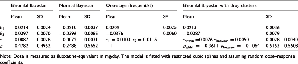
Note: Dose is measured as fluoxetine-equivalent in mg/day. The model is fitted with restricted cubic splines and assuming random dose–response coefficients.
In Figure 3 we present the absolute response using the binomial Bayesian model. The response in the placebo arm was estimated at 37.6% (blue line in Figure 3). We conducted a meta-analysis to synthesize evidence from studies of each drug separately, and we also present the absolute response for all drugs together. The precision in the dose–response curve is high for lower doses and increases for higher doses, as less data are available.
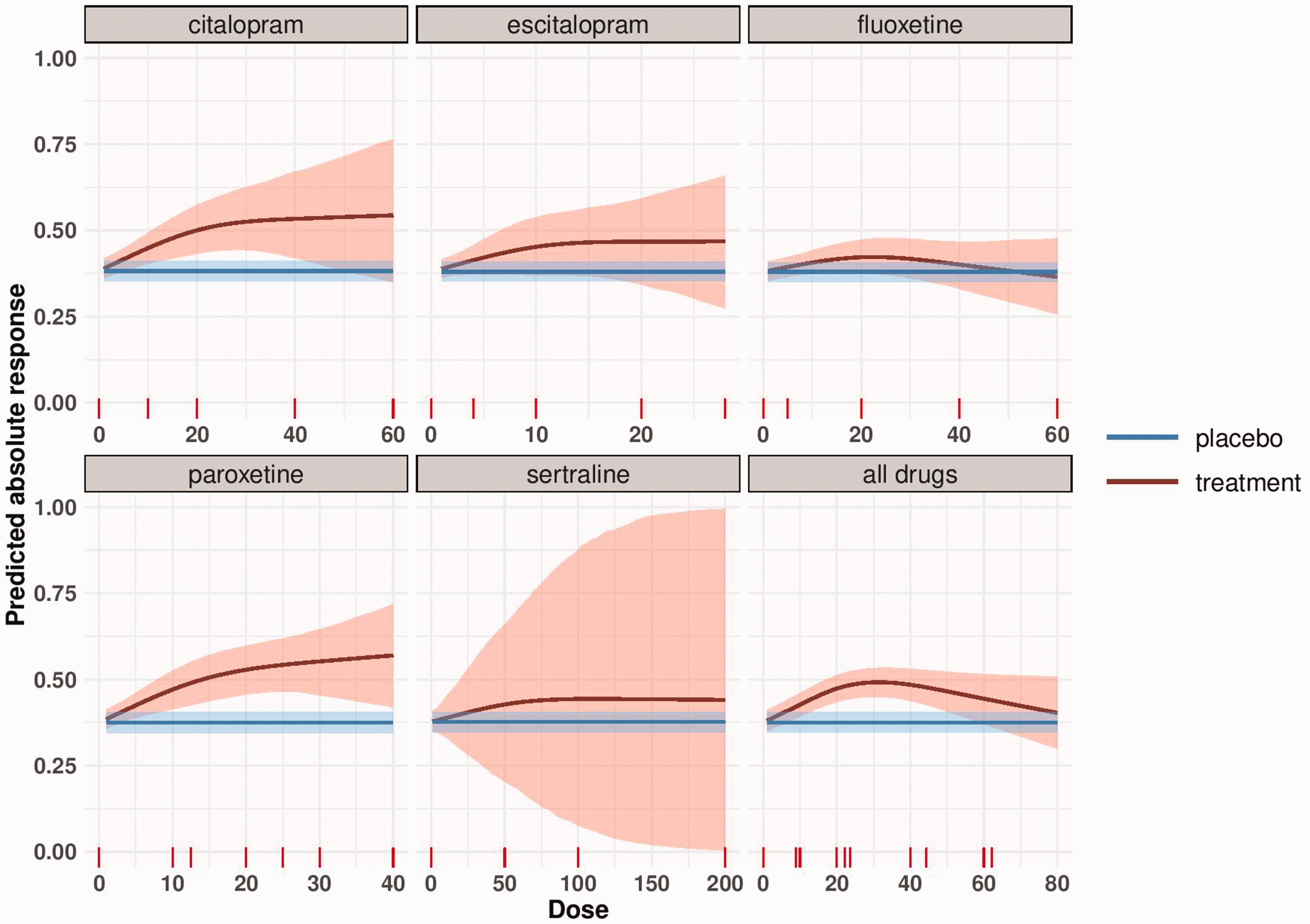
Dose–response meta-analysis of each SSRI and meta-analysis of all drugs with transformed doses (to fluoxetine-equivalent). The blue line represents the response to placebo as obtained by a meta-analysis of all placebo-arms and its 95% credible region. The red line depicts the absolute response to each antidepressant by dose estimated using the binomial Bayesian model. The shaded area represents the 95% credible region around the absolute dose–response curve.
We also fit the clustered dose–response model where studies have first been synthesized within drugs and then across drugs using the binomial likelihood. The coefficients
We examined the convergence of MCMC for all Bayesian models. Overall, convergence is achieved for all the estimated parameters of the three models, see supplementary Appendix Tables 11 to 16 and supplementary Appendix Figures 18 to 30.
5 Discussion
In this paper, we present a hierarchical dose–response meta-analysis model in a Bayesian framework. At the first level, the dose–response relationship is fitted within each study. Then the curves are combined to get the average dose–response. An additional pooling level can be added, if there are different clusters of exposure or drugs. The exact likelihood of the outcome (binomial or normal) can be employed if arm-level data is available.
We performed extensive simulations under different scenarios, in the majority of which the three tested models (binomial Bayesian, normal Bayesian and one-stage frequentist model) perform equally well and provide unbiased results. When the study sample size is small, we showed that the binomial Bayesian model performs better than the Bayesian or frequentist models that use normal likelihood. This is to be expected because with small sample size the observed logORs are poorly approximated by the normal distribution. One could use a logistic regression to model dose–response within a study; that would provide results equivalent to the binomial Bayesian approach. However, to the best of our knowledge, this approach has not been implemented in any frequentist software. When restricted cubic splines are used to model the association, we showed that prior knowledge about the underlying dose–response shape can direct the choice of the knot location and improve estimation.
Some articles have previously described methods for dose–response meta-analyses.7,8,11,34,35 Langford et al. proposed four methods to conduct dose–response meta-analysis in a frequentist setting. 34 The first two methods focus on the synthesis of arm-level responses which is undesirable in a meta-analysis context, in particular when randomized trials are synthesized. Method 3 is a one-stage approach; the contrasts between the arms are treated as observations to fit the dose–response curve using weighted least squares. Method 4 is a two-stage approach. In the first stage, all possible dose contrasts and their variances are estimated using network meta-analysis (where doses are placed in the network nodes). In the second stage, the obtained dose-specific estimates are used to fit the dose–response curve. Although Methods 3 and 4 are proposed to conduct the analysis based on contrasts, they ignore the correlations between them.
Wu et al. proposed a Bayesian hierarchical dose–response meta-analysis approach. 35 The approach aimed to examine the effects of various drugs extracted from living organism (biologics). The analysis was conducted assuming Emax and linear dose–response shapes. Such shapes are common in dose-findings trials. Our approach is, however, more general, in the sense that it can accommodate any dose–response shape. Our approach, additionally, considers both random- and common-effect models, whereas only the latter is considered by Wu et al. Allowing for heterogeneity between studies can be crucial as illustrated by Shi et al. who showed that the associations between breast cancer and alcohol consumption gets substantially weaker when the heterogeneity is incorporated in the model. 36
Among the limitations common to all Bayesian approaches, two are particularly challenging for our model.12,17 First, for some scenarios, the estimation can be sensitive to the prior choice. 37 In these cases, sensitivity analysis is recommended with either different prior distributions or by varying the characteristics (hyperparameters) of the specific prior distribution. This is particularly important for the heterogeneity parameter when we have few studies or dose levels. 37 Second, time-consuming, intensive computation may be required until MCMC convergence is achieved. In this context, we emphasize the importance of investigating the convergence of MCMC using CODA approaches (e.g. as those presented in our supplementary Appendix). Furthermore, the usual challenges of dose–response meta-analysis apply, including ambiguity in the categorization of the exposure, and the reporting of different categories by different studies or of open-ended categories. 38 These issues are discussed in detail elsewhere. 18 Finally, important considerations are to be made, that are specific to the data and context, when the (often continuous) dose has been categorized. 39
Simulations under a half-sigmoid and log–log dose–response shape revealed that an agnostic placement of the knots (e.g. in quantiles) might lead to biased and very imprecise estimation. Govindarajulu et al. also showed that restricted cubic splines can’t always capture the true shape. 40 Restricted cubic splines can perform poorly when most of the change in response is occurring in a narrow exposure interval and knots are located far away from it. In such scenario, subject-matter knowledge can inform the generation of restricted cubic splines by placing the knots where the investigator can anticipate most of the effect to occur, while keeping constant the number of parameters to be estimated. In meta-analysis of dose–response, investigators often know or suspect the underlying dose–response shape or at least the range of doses where the outcome is changing a lot. This should be incorporated in the assumed shape of the modelled dose–response association (e.g. by choosing a piecewise constant) or by locating the knots where changes are expected. In our example of antidepressants, psychiatrists would be interested about the shape in doses lower than 50 mg fluoxetine-equivalent and changes in response are expected to occur between 20 and 40 mg (the minimum therapeutic dose). Therefore, knots have to be placed at these dosages.
A strength of our Bayesian approach is its flexibility. We were able to evaluate whether studies that examine the same drug are more similar than studies examining different drugs by using an extension of our model that adds a layer in the hierarchy according to the specific kind of antidepressant that was studied. We were also able to estimate the absolute response to each dose. Such estimates can also be obtained in a frequentist setting by using best linear unbiased prediction (BULPs) in mixed models.41,42 However, the process is easier in a Bayesian framework, which also allows the use of external data to estimate the outcome at zero dose. The approach will be particularly valuable in the context of policy- and decision-making where the absolute event rates play a more important role than the relative treatment effects.
The hierarchical structure of the model allows the borrowing of strength across studies. 14 Studies that report only one dose-specific effect can thus be included and a nonlinear dose–response model fitted. This is also possible in a frequentist setting using the one-stage approach; however, our model can be extended to separate between the heterogeneity due to variability in dose–response shape and residual between-study heterogeneity. The latter can be explored by including covariates that may explain this residual variability, which could lead to a dose–response meta-regression. Our model could also be extended to multiple treatments, thus offering an alternative to published network meta-analysis models, 43 or it could be used to model simultaneously several outcomes with similar dose–response shapes. Another potential extension, which we have implemented in our paper, is accounting for cluster of the exposure in estimating the dose–response shape. Finally, external knowledge can be incorporated, for example, evidence from observational studies. The use of observational data will be particularly relevant when assessing long-term outcomes, as the majority of RCTs, in psychiatry and elsewhere, are of relatively short duration. 17
In conclusion, we suggest that the Bayesian model with the binomial likelihood could be the default approach as it outperforms the alternative models when the synthesized studies are small. Prior knowledge about the underlying association should be incorporated in the model by defining an appropriate dose–response shape or by locating knots at doses where the outcome is expected to change a lot.
Supplemental Material
sj-pdf-1-smm-10.1177_0962280220982643 - Supplemental material for A Bayesian dose–response meta-analysis model: A simulations study and application
Supplemental material, sj-pdf-1-smm-10.1177_0962280220982643 for A Bayesian dose–response meta-analysis model: A simulations study and application by Tasnim Hamza, Andrea Cipriani, Toshi A Furukawa, Matthias Egger, Nicola Orsini and Georgia Salanti in Statistical Methods in Medical Research
Footnotes
Authors’ Note
Andrea Cipriani and Matthias Egger are also affiliated with Oxford Health NHS Foundation Trust, Warnford Hospital, Oxford, UK and Population Health Sciences, Bristol Medical School, University of Bristol, Bristol, UK, respectively.
Acknowledgements
The authors would like to acknowledge two anonymous reviewers who made very helpful comments and suggestion to this work. The views expressed are those of the authors and not necessarily those of the UK National Health Service, the NIHR, or the UK Department of Health.
Declaration of conflicting interests
The author(s) declared the following potential conflicts of interest with respect to the research, authorship, and/or publication of this article: Andrea Cipriani has received research and consultancy fees from INCiPiT (Italian Network for Paediatric Trials), CARIPLO Foundation and Angelini Pharma. The other authors declared no potential conflicts of interest with respect to the research, authorship, and/or publication of this article.
Funding
The author(s) disclosed receipt of the following financial support for the research, authorship, and/or publication of this article: TH and GS were funded by the European Union’s Horizon 2020 research and innovation programme under grant agreement No 825162. ME was supported by a special project funding from the Swiss National Science Foundation (grant no. 17481). AC is supported by the National Institute for Health Research (NIHR) Oxford Cognitive Health Clinical Research Facility, by an NIHR Research Professorship (grant RP-2017-08-ST2-006), by the NIHR Oxford and Thames Valley Applied Research Collaboration and by the NIHR Oxford Health Biomedical Research Centre (grant BRC-1215-20005).
Supplemental material
Supplemental material for this article is available online.
References
Supplementary Material
Please find the following supplemental material available below.
For Open Access articles published under a Creative Commons License, all supplemental material carries the same license as the article it is associated with.
For non-Open Access articles published, all supplemental material carries a non-exclusive license, and permission requests for re-use of supplemental material or any part of supplemental material shall be sent directly to the copyright owner as specified in the copyright notice associated with the article.