
Abstract
It is widely recommended that any developed—diagnostic or prognostic—prediction model is externally validated in terms of its predictive performance measured by calibration and discrimination. When multiple validations have been performed, a systematic review followed by a formal meta-analysis helps to summarize overall performance across multiple settings, and reveals under which circumstances the model performs suboptimal (alternative poorer) and may need adjustment. We discuss how to undertake meta-analysis of the performance of prediction models with either a binary or a time-to-event outcome. We address how to deal with incomplete availability of study-specific results (performance estimates and their precision), and how to produce summary estimates of the c-statistic, the observed:expected ratio and the calibration slope. Furthermore, we discuss the implementation of frequentist and Bayesian meta-analysis methods, and propose novel empirically-based prior distributions to improve estimation of between-study heterogeneity in small samples. Finally, we illustrate all methods using two examples: meta-analysis of the predictive performance of EuroSCORE II and of the Framingham Risk Score. All examples and meta-analysis models have been implemented in our newly developed R package “metamisc”.
Keywords
1 Introduction
In medicine, many decisions require to estimate the risk or probability of an existing disease (diagnosis) or of developing a future outcome that yet has to occur (prognosis). Although having experience and intuition often provide excellent advice, it is increasingly common to quantify such diagnostic and prognostic probabilities through the use of prediction models. These models commonly combine information from multiple findings, such as from history taking, physical examination, and additional testing such as blood, imaging, elektrofysiology, and omics tests, to provide absolute outcome probabilities for a certain individual. Prediction models can, for instance, be used to inform patients and their treating physicians, to decide upon the administration of subsequent testing (diagnostic models) or treatments (prognostic models), or to identify participants for clinical trials.1,2 Well-known examples are the European system for cardiac operative risk evaluation (EuroSCORE) II to predict mortality after cardiac surgery 3 and the Framingham Risk Score for predicting coronary heart disease. 4
Over the past few decades, prediction modeling studies have become abundant in the medical literature. For the same disease, outcome or the target population, often numerous, sometimes hundreds, prediction models have been published. 5 This practice is clearly undesirable for health-care professionals, guideline developers and patients, as it obfuscates which model to use in which context. More efforts are therefore needed to evaluate the performance of existing models in new settings and populations, and to adjust them if necessary. 6 In contrast to redevelopment, validation and updating of prediction models allows to (more effectively) account for information already captured in previous studies, and thus to make better use of existing evidence and data at hand.7,8
The evaluation (and revision) of prediction models can be achieved by performing so-called external validation studies. In these studies, the original model is applied to new individuals whose data were not used in the model development. Model performance is then assessed by comparing the predicted and observed outcomes across all individuals, and by calculating measures of discrimination and calibration. Discrimination quantifies a model’s ability to distinguish individuals who experience the outcome from those who remain event free, while calibration refers to the agreement between observed outcome frequencies and predicted probabilities. Unfortunately, the interpretation of validation study results is often difficult, as changes in prediction model performance are likely to occur due to sampling error, differences in predictor effects, and/or differences in patient spectrum.9,10 Furthermore, because validation studies are often conducted using small and local data sets, 11 they rarely provide evidence about a model’s potential generalizability across different settings and populations. For this reason, it may come as no surprise that for many developed prediction models, numerous authors have (re-)assessed the discrimination and calibration performance. Systematic reviews—ideally including a formal meta-analysis—are thus urgently needed to summarize their evidence and to better understand under what circumstances developed models perform adequately or require further adjustments.
Previous guidance for systematic reviews of prediction model studies mainly addressed formulation of the review aim, searching, 12 critical appraisal (CHARMS) 13 and data extraction of relevant studies. There is, however, little guidance on how to quantitatively synthesize the results of external validation studies. For this reason, we recently discussed meta-analysis methods to summarize and examine a model’s predictive performance across different settings and (sub)populations. 14 These methods mainly focused on (diagnostic) prediction models with a binary outcome, and may therefore have limited value when reviewing (prognostic) models with a time-to-event outcome.
For this reason, we provide a comprehensive statistical framework to meta-analyze performance estimates of both diagnostic and prognostic prediction models, involving either binary or time-to-event outcomes. In particular, we discuss how to extract and restore relevant (and possibly missing) estimates of prediction model performance, and corresponding estimates of uncertainty. We also discuss how to obtain summary estimates of discrimination and calibration performance, even when none of the primary studies reported such estimates. Finally, we discuss the role and implementation of Bayesian methods for meta-analysis, and contrast their use with the more traditional frequentist methods. We illustrate all methods by reanalyzing the data from previously published reviews involving a prediction model with a binary 3 and with a time-to-event 4 outcome. All methods have been implemented in the R package “metamisc”, which is available from https://CRAN.R-project.org/package=metamisc. 15 This package aims to facilitate meta-analysis of prediction model performance by integrating the proposed statistical methods for data extraction and evidence synthesis.
2 Motivating examples
We here focus on prediction models with either a binary or time-to-event outcome, as these are most common in the medical literature. 16 Binary outcomes are typically used to represent the current (health) status of an individual, or to model events that occur within a relatively short period of time. Examples include the presence or absence of a particular disease, or death after surgery. Conversely, when the event times are of primary interest, binary outcomes need to be modeled together with the time after which they occurred. Examples of these so-called time-to-event outcomes include the time until the onset of breast cancer, the time until cardiovascular death, or the time until development of coronary heart disease (CHD).
Population, intervention, comparison, outcome, timing and setting (PICOTS) of the empirical examples.
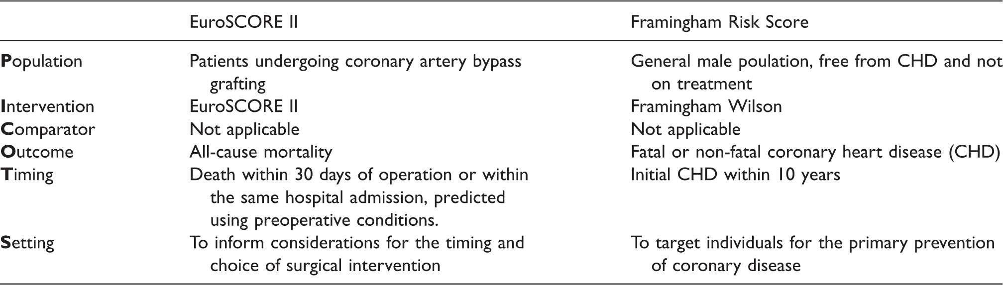
In the first example, we meta-analyze the predictive performance of the European system for cardiac operative risk evaluation (EuroSCORE) II. This logistic regression model was developed using 16,828 adult patients from 43 countries to predict mortality after cardiac surgery. 3 The corresponding prediction model equations are presented in Supporting Information 1.1. In a recent review, 17 23 validations of EuroSCORE II were identified in which its predictive performance was examined in patients undergoing cardiac surgery. For each study, the number of patients, their mean age, and the proportion of female gender were extracted, as well as information on mortality, the concordance (c-) statistic, and the EuroSCORE II mean value. All data are available from the R package “metamisc”.
In the second example, we meta-analyze the predictive performance of the Framingham Risk Score developed by Wilson et al. 4 This Cox proportional hazards regression model was developed in 1998 for predicting the 10-year risk of CHD in the general population free from CHD and not on treatment (Supporting Information 1.2). A recent systematic review identified 23 studies examining the performance of Framingham Wilson for predicting fatal or nonfatal CHD in male populations (Supporting Information 1.2). 18 For each validation, estimates of model calibration and discrimination were extracted, as well as details on the study and population characteristics.
3 Data extraction and estimating unreported results to facilitate meta-analysis
The two most common statistical measures of predictive performance are described by discrimination and calibration. In a meta-analysis without access to individual participant data (IPD), we are reliant on extracting these performance measures from study publications. However, they are often poorly reported.11,16 We now discuss how to retrieve the necessary but not explicitly reported predictive performance estimates from the primary prediction model (validation) studies using other reported data.
3.1 Model discrimination
Discrimination refers to a prediction model’s ability to distinguish between subjects developing and not developing the outcome, and is often quantified by the concordance (c)-statistic, both for prediction models for binary outcomes as well as for time-to-event outcomes. The c-statistic is an estimated conditional probability that for any pair of a subject who experienced and a subject who did not experience the outcome, the predicted risk of an event is higher for the former. Although c-statistics are frequently reported in external validation studies, when missing they can also be calculated from other reported quantities. For instance, for prediction models with a binary outcome, the c-statistic is a reparameterization of Somer’s D, 19 and can also be derived from the distribution of the linear predictor, 20 Cohen’s effect size, 20 or several correlation indices. 21 An overview of relevant equations for this derivation of the c-statistic from other measures was previously presented. 14
In this study, we compared two methods for estimating the c-statistic from reported information. Results in Supporting Information 2.2 indicate that accurate predictions can be obtained for c < 0.70 by using the standard deviation of the linear predictor. More accurate predictions (for c < 0.95) can be obtained if the mean and variance of the linear predictor are known for the affected and unaffected populations.
For prediction models with a time-to-event outcome, concordance is not uniquely defined and several variations of the c-statistic have been proposed.22,23 These variations typically adopt different strategies to account for ties or censoring, and may thus lead to different values for c. Although validation studies do not commonly report the definition and estimation method of presented c-statistics, Harrell’s version
21
appears to be most widespread and recommended.
22
Sometimes, discrimination is measured using Royston and Sauerbrei’s D index, usually referred to as the “D statistic”.
24
This index quantifies prognostic separation of survival curves and is closely related to the standard deviation of the prognostic index, with Jinks et al. suggesting an equation to convert c values to D values based on empirical evidence
25

It is also possible to convert D values to c values by making distributional assumptions with respect to the standard deviation of the prognostic index.
26
The c-statistic can then be predicted as follows

For prediction models including covariates with time-dependent effects and/or time-dependent covariates, concordance is often measured using time-dependent ROC curves. 27 Again, several variations have been proposed that adopt different strategies to account for censoring. A recent study by Blanche et al. showed that these strategies perform similarly when censoring is independent, 28 and are thus likely to yield comparable estimates of time-dependent concordance. However, when censoring depends on the predictor values, some ROC curve estimators are prone to substantial bias and may therefore contribute towards between-study heterogeneity in a meta-analysis.
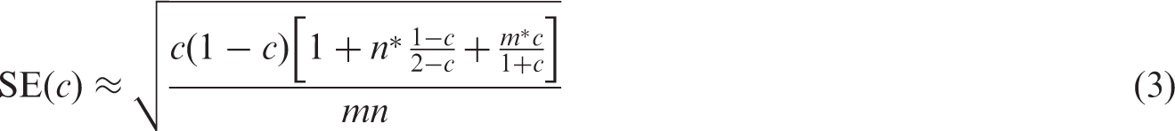
Regarding the standard error of the c-statistic, when missing, it can be approximated from a combination of the reported c-statistic, the total sample size and the total number of events in the validation study. We here consider a method proposed by Newcombe to estimate the standard error of the c-statistic.
29
As we will discuss in the next section, it is important to transform estimates of the c-statistic and its standard error to the logit scale prior to meta-analysis.
30
The logit c-statistic is simply given by 
Alternatively, when the lower (
3.2 EuroSCORE II
Estimates for the c-statistic could be obtained for all 23 validations (Supporting Information 1.1). For four validations, equation (4) was used to approximate the standard error of the (logit) c-statistic. An example is given below.
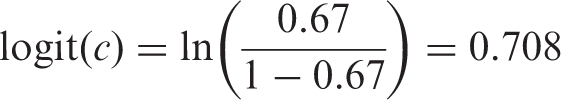
Previously, Howell et al. assessed the predictive performance of EuroSCORE II in 933 high-risk patients.
33
The observed in-hospital mortality was 9.7% (90 deaths). The reported c-statistic was 0.67; however, no information was provided on the corresponding standard error or confidence interval. We can derive the logit c-statistic as follows
Further, based on the reported information, we have n = 90, m = 843 and 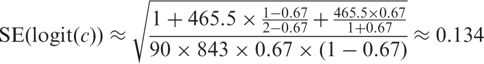
3.3 Framingham
The c-statistic was only reported in 19/24 validations. In some cases, missing c-statistics could be restored by contacting the study authors (two validations). For these 21 estimates of the c-statistic, 10 studies provided the standard error and 11 studies required approximation of the standard error using Newcombe’s method (Supporting Information 1.2).
3.4 Model calibration
Calibration refers to a model’s accuracy of predicted probabilities, and is preferably reported graphically in so-called calibration plots. In these plots, expected outcome probabilities from the model are depicted against observed outcome frequencies in the validation dataset, often across tenths of predicted risk or for 4–5 risk groups over time (e.g. via Kaplan–Meier plots versus predicted survival). Calibration plots can also be constructed using smoothed loess curves, by directly regressing (transformations of) expected versus observed outcomes.
In order to summarize a model’s calibration performance across different validation studies, it is helpful to retrieve expected and observed outcome probabilities (e.g. across different risk strata), and to extract reported calibration measures. For prediction models for binary outcomes as well as for time-to-event outcomes, common measures are the calibration intercept and slope. 34 The intercept is also known as calibration-in-the-large, and indicates whether predicted probabilities are, on average, too high (intercept below 0) or too low (intercept above 0). Conversely, the calibration slope quantifies whether predicted risks are, on average, too extreme (slope below 1) or too invariant (slope above 1). 35
Unfortunately, extraction of calibration measures is often hampered by poor assessment and reporting.11,16 For instance, validation studies rarely present information on the calibration intercept and slope, or different studies report estimates for different risk strata or time horizons. However, it is common for validation studies to present information on the total number of observed (O) and expected (E) events, or the corresponding observed frequencies
For prediction models with a time-to-event outcome, it is important to be aware that some events are likely to be unobserved (e.g. due to drop-out). For this reason, extracted values for O (or
Further, as we will discuss in the next section, estimates of the total 
Formulas for estimating the total
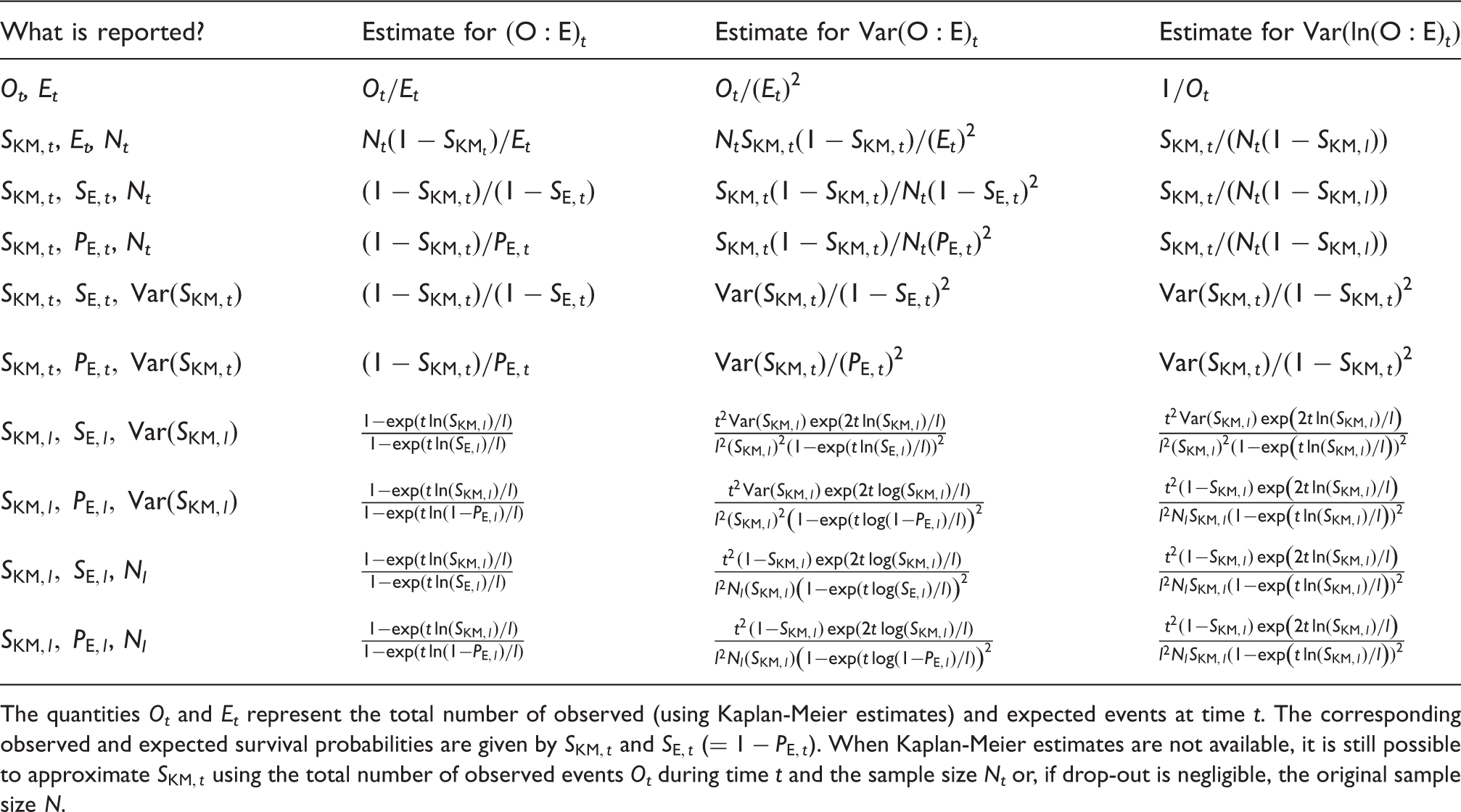
The quantities Ot and Et represent the total number of observed (using Kaplan-Meier estimates) and expected events at time t. The corresponding observed and expected survival probabilities are given by
Although the total
3.5 Example
Buitrago et al. analyzed the 10-year performance of the original Framingham coronary risk functions in nondiabetic patients.
37
They reported the observed (

3.6 Framingham
Estimates for observed and expected 10-year CHD risk were directly available for 6/24 validations (Supporting Information 1.2). For some studies,
3.7 EuroSCORE II
The total number of observed and expected events was available for all 23 validations. Furthermore, because the EuroSCORE II model does not consider time-to-event, estimates for the total
4 Meta-analysis
Once all relevant studies have been identified and corresponding results have been extracted, the retrieved estimates of model discrimination and calibration can be summarized into a weighted average to provide an overall summary of their performance. We here consider the situation where K studies (
4.1 Meta-analysis models
In general, two main types of meta-analysis models can be distinguished. In fixed effect meta-analysis models, all studies are considered to be equivalent, and variation in predictive performance measures across studies are assumed to arise by chance only. Accordingly, precision estimates of discrimination and calibration parameters are used to weight each study in the averaging of the model’s corresponding performance measures. In random effects meta-analysis models, it is assumed that variation in predictive performance measures across studies may not only appear due to chance, but is also prone to the (potential) presence of between-study heterogeneity. As a result, random effects models usually yield larger confidence intervals and assign study weights that are more similar to one another than those under fixed effect meta-analysis. 40
Although both types of aforementioned meta-analysis models have limitations, and following the guidance of meta-analysis of interventions and diagnostic tests, we generally recommend the use of random effects models. In particular, discrimination and calibration performance are highly dependent on patient spectrum (case-mix variation) and therefore most likely to vary across validation studies. 14 For instance, it is well known that a model’s discrimination performance tends to deteriorate when it is applied to populations or subgroups with a more homogeneous case-mix, as there is less separation of predicted risks across individuals.9,10,20,41,42 Between-study heterogeneity may also appear when reported performance estimates (such as c-statistics) are based on different definitions or estimation methods (e.g. adopt different criteria to account for ties or censoring).
4.2 Model discrimination
For random effects meta-analysis of the c-statistic (for either logistic or survival models), we have

4.3 Model calibration
Similarly, for random effects meta-analysis of the total 
One approach to avoid continuity corrections is to explicitly account for sampling error in the observed event rates by modelling the binomial likelihood directly in a one-stage random-effects model, where the within and between-study distributions are modelled in a single analysis
43
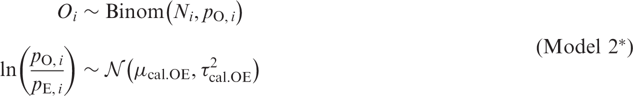
Alternatively, we may treat the total number of observed events as count data in a one-stage random-effects model
43

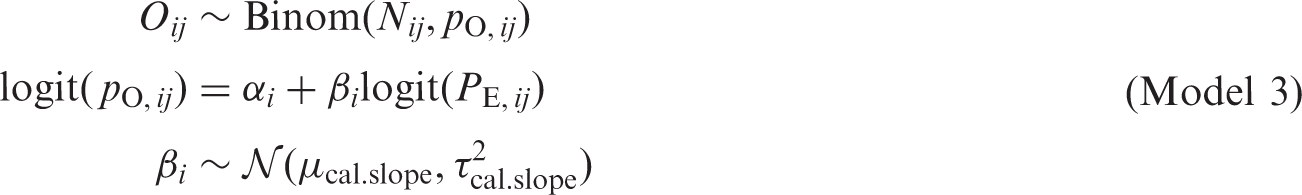
Finally, if observed and expected event rates are available for different strata of predicted risk in the validation studies, it is possible to obtain a summary estimate of the calibration slope (Supporting Information 4.4.3). The one-stage random effects model below is a natural extension of Cox’ proposed regression model for describing agreement between predicted and observed probabilities
35
4.4 The frequentist approach for random effects meta-analysis
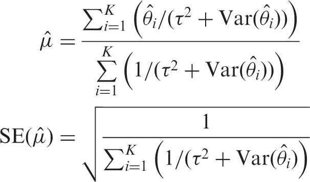
The parameters of the meta-analysis models above (Models 1 and 2) can be estimated by optimizing their corresponding (log-)likelihood function. This yields the well-known estimator of the meta-analysis summary
44
In line with previous recommendations,46,47 we propose to correct estimates of 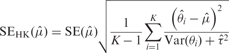
For all models, boundaries of the confidence interval (CI) can then be approximated using
Finally, for meta-analysis of model discrimination and calibration, we recommend the calculation of an (approximate) 95% prediction interval (PI) to depict the extent of between-study heterogeneity.
48
This interval provides a range for the predicted model performance in a new validation of the model. A 95% PI for the summary estimate in a new setting is approximately given as
4.5 The Bayesian approach for random effects meta-analysis
Generally speaking, in contrast to frequentist methods, Bayesian methods use formal probability models to express uncertainty about parameter values.49,50 This is particularly relevant when confronting sparse data, multiple comparisons, collinearity, or non-identification, and for deriving PI. 51 Estimation problems are likely to occur in frequentist meta-analyses of prediction model performance, as validations of a specific model and thus existing evidence or data on predictive performance measures are often sparse. Furthermore, many frequentist estimation methods (including REML) sometimes fail to produce reliable confidence or prediction intervals. For instance, Partlett and Riley showed that the coverage of Hartung–Knapp confidence intervals based on REML estimation is too narrow for meta-analyses with less than five studies. 46 Furthermore, when the heterogeneity is small and the study sizes are mixed, the Hartung–Knapp method produces confidence intervals that are too wide.46,47 Similarly, prediction intervals have poor coverage when the extent of heterogeneity is limited, when few (less than 5) studies are included, or when there are a mixture of large and small studies. 46 For this reason, several authors have recommended the adoption of a Bayesian estimation framework,46,52,53 which more naturally accounts for all parameter uncertainty in the derivation of credibility and probability intervals.
An additional advantage of Bayesian meta-analysis models is that the distribution for modeling the within-study variation can be tailored to each validation study. This is, for instance, relevant when meta-analyzing the total
When adopting a Bayesian framework for meta-analysis, it is always important to specify appropriate prior distributions. In aforementioned meta-analysis models, prior distributions are needed for the unknown parameters
Results in Supporting Information 4.2 demonstrate that for the logit c-statistic and the log
Because the uniform distribution tends to unduly favor presence of heterogeneity in discrimination and calibration estimates across studies,58,59 we also consider a half Student-t distribution with location m, scale σ and ν degrees of freedom. Here, we set m = 0 and define σ equal to the largest empirical value of
To evaluate the performance of the proposed prior distributions, we used the empirical example data to conduct a series of simulation studies where we varied the size of the meta-analysis (Supporting Information 4.5). Results in Figure 1 and Figure 2 suggest that the proposed priors substantially improve estimation of the between-study standard deviation when meta-analyses are relatively small. Researchers may, however, need to further tailor these priors to their own particular setting and example.
Estimation of 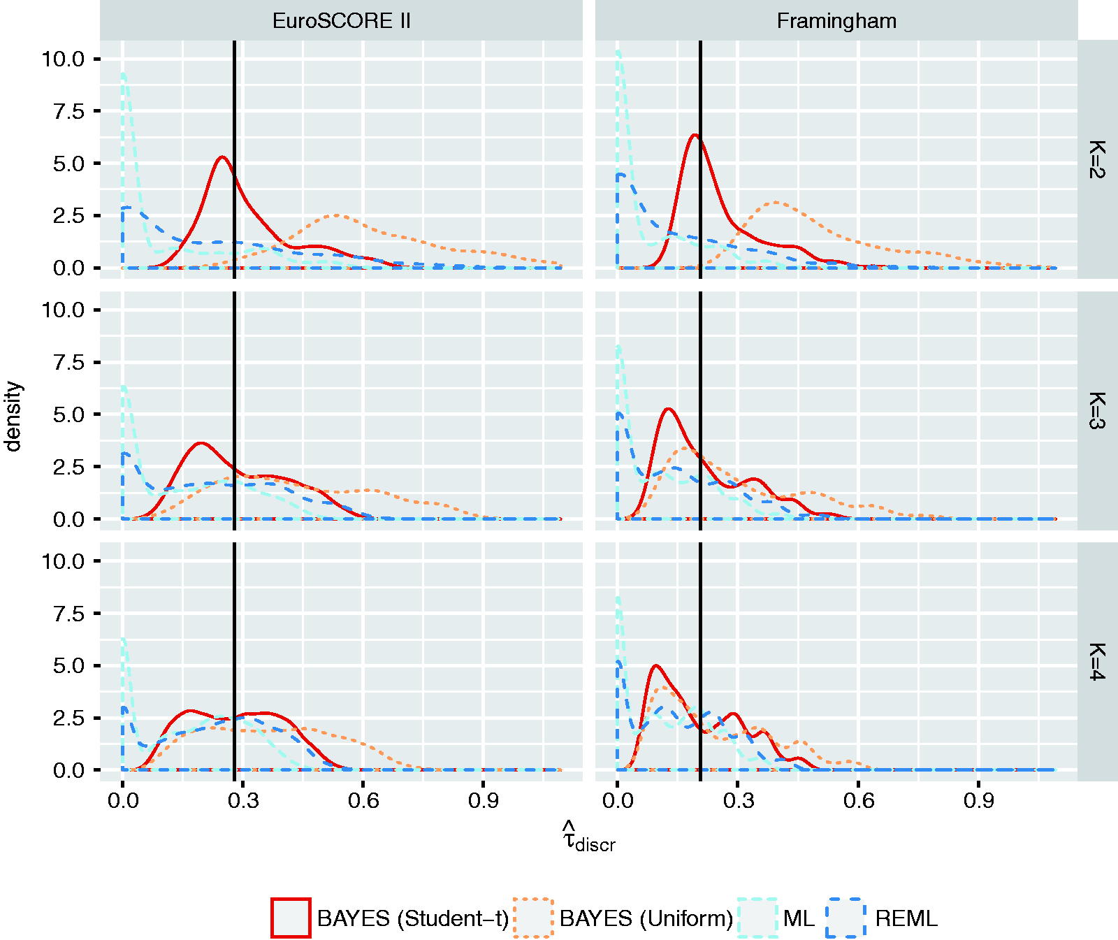
To further highlight the potential advantages of Bayesian meta-analysis, we extended Model 3 to directly account for (1) sampling error in the number of expected events, (2) uncertainty due to the need for extrapolation and (3) uncertainty resulting from data transformations. The corresponding Model 3* is given in Supporting Information 4.4.3, and may help to conduct sensitivity analyses.
Finally, similar to a frequentist meta-analysis, uncertainty around summary estimates resulting from sampling error and/or heterogeneity can be formally quantified. In a Bayesian meta-analysis, the corresponding intervals are denoted as credibility and, respectively, prediction intervals. Boundaries for these intervals can directly be obtained by sampling from the posterior distribution. 51 It is also possible to make probabilistic statements about future validation studies, such as the probability that the c-statistic will be above 0.7, or that the calibration slope will be between 0.9 and 1.1.
4.6 Empirical examples
All meta-analysis models have been implemented in the R-package “metamisc”. Convergence of Bayesian meta-analysis models was verified by evaluating the upper confidence limits of the potential scale reduction factor (values
4.7 EuroSCORE II
Meta-analysis estimates for the EuroSCORE II model.
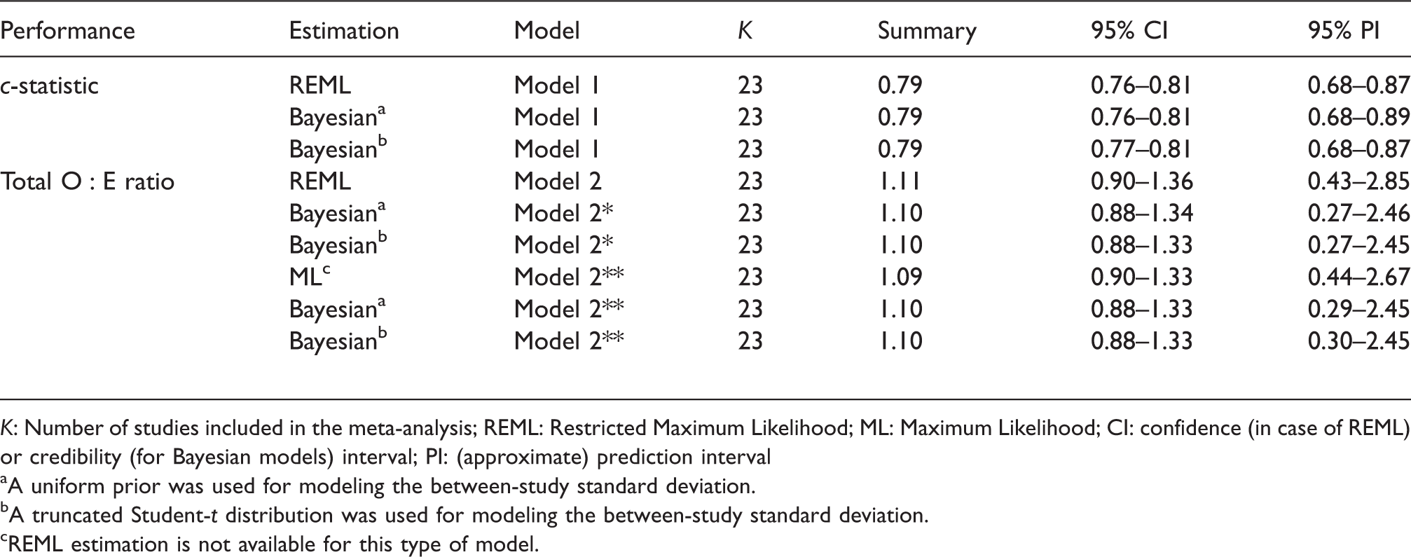
K: Number of studies included in the meta-analysis; REML: Restricted Maximum Likelihood; ML: Maximum Likelihood; CI: confidence (in case of REML) or credibility (for Bayesian models) interval; PI: (approximate) prediction interval
A uniform prior was used for modeling the between-study standard deviation.
A truncated Student-t distribution was used for modeling the between-study standard deviation.
REML estimation is not available for this type of model.
To illustrate the potential advantages of hierarchical related regression, we omitted information on the total sample size for seven studies. Model 2* could then only be applied to 16 studies, yielding a summary estimate for the total Estimation of Meta-analysis estimates for EuroSCORE II.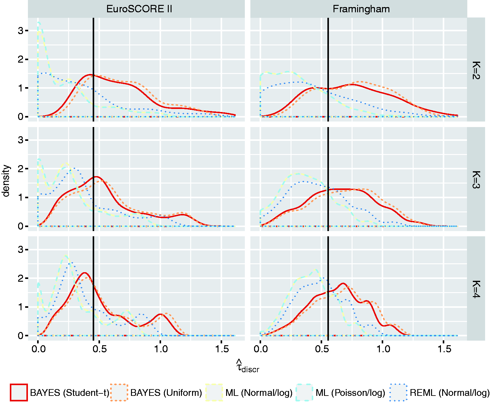
4.8 Framingham
Meta-analysis estimates for the Framingham Risk Score.
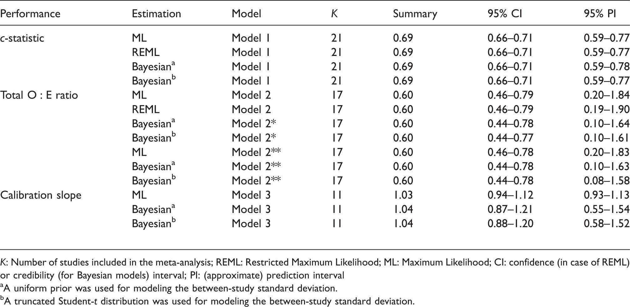
K: Number of studies included in the meta-analysis; REML: Restricted Maximum Likelihood; ML: Maximum Likelihood; CI: confidence (in case of REML) or credibility (for Bayesian models) interval; PI: (approximate) prediction interval
A uniform prior was used for modeling the between-study standard deviation.
A truncated Student-t distribution was used for modeling the between-study standard deviation.
5 Investigating sources of heterogeneity
As applies to all types of meta-analysis, also for meta-analysis of prediction model studies, summary estimates of model performance may be of limited value in the presence of (substantial) between-study heterogeneity. Although we recommended the use of random effects models to evaluate the presence of heterogeneity, these models do not offer any insight about potential causes of this. For this reason, it is often helpful to investigate potential sources of heterogeneity in the predictive performance by performing a meta-regression or subgroup analysis.14,61 Common sources of heterogeneity are differences in study characteristics, 62 differences in study quality, or differences in baseline risk across the validation studies.9,10 Heterogeneity may also arise when reported performance estimates are based on “improper” validations where certain predictors were neglected (e.g. due to missing data) or where various model parameters have been adjusted (e.g. intercept update).
5.1 Meta-regression models
We extend the presented meta-analysis models as follows to investigate sources of between-study heterogeneity.
63
Let 
To enhance estimation of covariate effects
5.2 Empirical examples
We used the R-package “metafor” to estimate the meta-regression models.
5.3 EuroSCORE II
In a meta-regression model (for discrimination), we examined whether heterogeneity was explained by one or more of the following: the spread of the prognostic index of EuroSCORE II in each validation study, whether the study was a multicentre study, whether the study included patients before 2010 (i.e. before EuroSCORE II was developed) and the spread of the age of the patients. The resulting meta-regression plots are depicted in Figure S14 (Supporting Information), and indicate that the summary c-statistic generally remains unaffected by changes in the distribution of the prognostic index or patient age. The p-value of the regression coefficients was all larger than 0.05. We therefore could not attribute heterogeneity in the c-statistic to these differences.
5.4 Framingham
We examined whether heterogeneity for the Framingham Risk Score in male populations could be explained by differences in age distribution, smoking prevalence, and observed 10-year event rates. For instance, the mean age ranged from 41 to 74 across the included validations. Also the standard deviation of age substantially varied across the included validation studies (range: 2–13), further highlighting the presence of differences in patient spectrum. Results in Figure 4 indicate that the c-statistic of the Framingham Risk Score tended to decrease when validated in older (male) populations (p = 0.01). This can be explained by the narrower case-mix leading to more narrow separation, and thus lower c values. For the calibration performance, we found that under-estimation (i.e. Results from random-effects meta-regression models for the Framingham Risk Score (validations in male populations). Full lines indicate the bounds of the 95% confidence interval around the regression line. Dots indicate the included validation studies.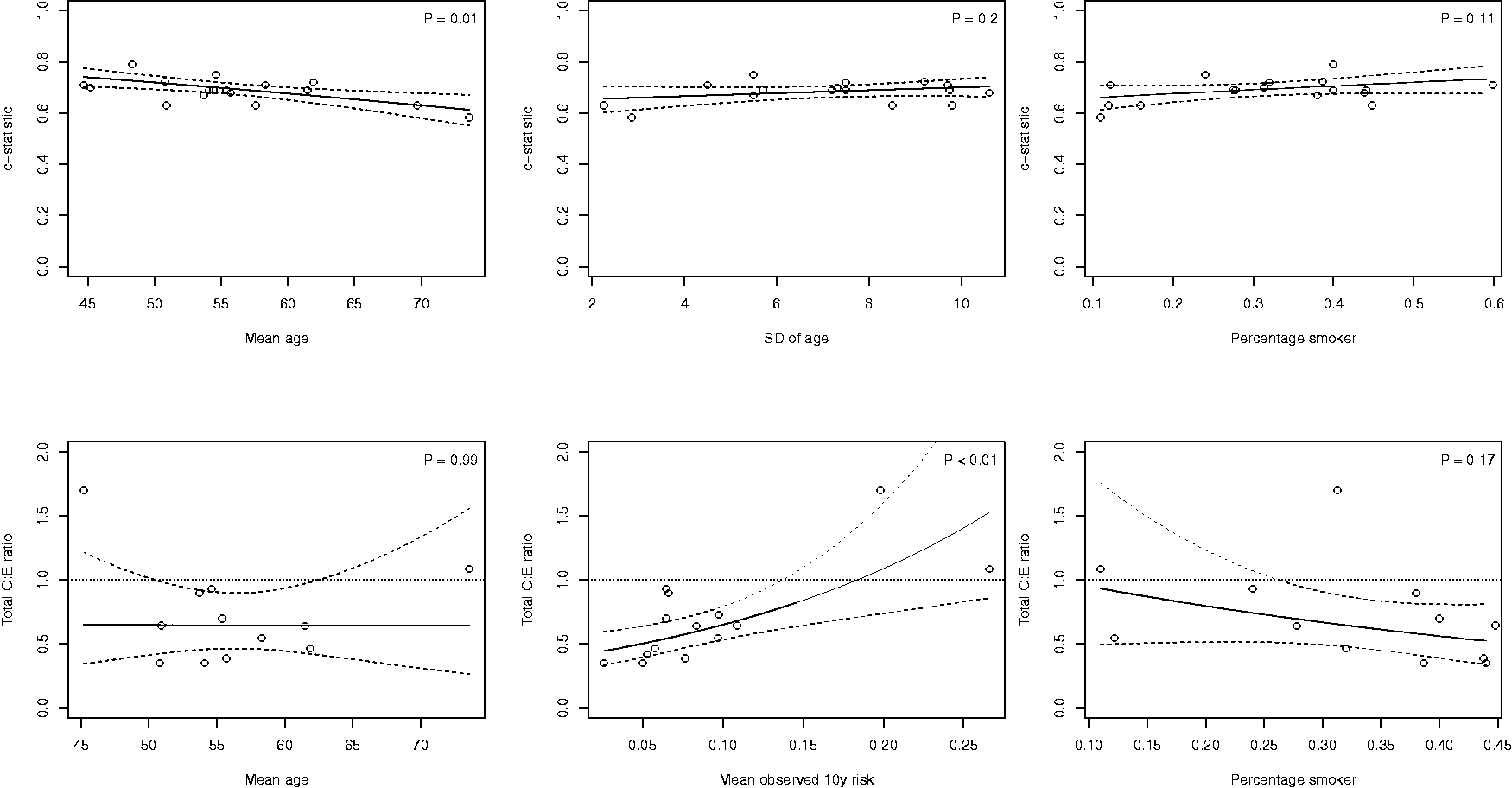
6 Conclusion
Quantitative synthesis of prediction model studies may help to better understand their potential generalizability and can be achieved by applying meta-analysis methods. 14 In this paper, we discussed several common stumbling blocks when meta-analyzing the predictive performance of prediction models. In particular, substantial efforts are often needed to restore missing information from the primary studies and to harmonize the extracted performance statistics. In addition, estimates of a model’s predictive performance are likely to be affected by the presence of between-study heterogeneity. Finally, because validation studies of a certain prediction model are often sparse, traditional (frequentist) meta-analysis models may suffer from convergence issues and yield unreliable estimates of precision and between-study heterogeneity. 64 For this reason, we presented several methods to overcome these deficiencies, and to obtain relevant summary statistics of prediction model performance even when the primary validation studies did not report such information. Furthermore, to facilitate the implementation of the presented methods, we created the open source R package metamisc which includes the empirical example data. 15
We generally recommend the use of one-stage methods for summarizing the O:E ratio (here, Model 2* and Model 2**) and calibration slope (here, Model 3), as they use the exact likelihood. Further, adopting a Bayesian estimation framework may help to fully propagate the uncertainty resulting from estimating the within-study standard errors and the between-study standard deviation, which in turn may improve the coverage of calculated intervals. Future efforts should focus on comparing the presented meta-analysis methods in new empirical examples and simulation studies. Results from previous studies suggest that these methods are most likely to yield discordance when there is low between-study heterogeneity, when there are few studies for meta-analysis, or when studies are small or based on different sample sizes.46,65,66
Further work is also still needed to summarize the evidence on multiple, competing, prediction models that were compared head-to-head in validation studies. Another important issue arises when individual participant data (IPD) are available for one or more validation studies. Although it is possible to reduce these studies to relevant performance estimates and to adopt the meta-analysis methods presented in this article, more advanced (so-called one-stage) approaches exist to directly combine the IPD with published summary data. 67 An additional advantage of IPD is that it becomes possible to adjust discrimination performance for (variation in) subject-level covariates, and thus to gain more understanding in sources of between-study heterogeneity.9,10,26,68 Finally, methods for meta-analyzing clinical measures of performance such as net benefit deserve further attention.
In summary, our empirical examples demonstrate that meta-analysis of prediction models is a feasible strategy despite the complex nature of corresponding studies. As developed prediction models are being validated increasingly often, and as the reporting quality is steadily improving, we anticipate that evidence synthesis of prediction model studies will become more commonplace in the near future. The R package “metamisc” is designed to facilitate this endeavor, and will be updated as new methods become available.
Supplemental Material
Supplemental material for A framework for meta-analysis of prediction model studies with binary and time-to-event outcomes
Supplemental Material for A framework for meta-analysis of prediction model studies with binary and time-to-event outcomes by Thomas PA Debray, Johanna AAG Damen, Richard D Riley, Kym Snell, Johannes B Reitsma, Lotty Hooft, Gary S Collins and Karel GM Moons in Statistical Methods in Medical Research
Footnotes
Acknowledgements
We gratefully acknowledge Ian White for sharing the algebraic expressions relating the c-statistic in terms of the standard deviation of the linear predictor (equation ![]() , and Supporting Information 2.2.1). Further, we thank Hans van Houwelingen for his reference to earlier work by D. R. Cox on the calibration slope.
, and Supporting Information 2.2.1). Further, we thank Hans van Houwelingen for his reference to earlier work by D. R. Cox on the calibration slope.
Declaration of conflicting interests
The author(s) declared no potential conflicts of interest with respect to the research, authorship, and/or publication of this article.
Funding
The author(s) disclosed receipt of the following financial support for the research, authorship, and/or publication of this article: The work leading to these results has received support from the Netherlands Organisation for Health Research and Development (91617050) and from the Cochrane Methods Innovation Funds Round 2 (MTH001F).
Supplemental material
Supplemental material for this article is available online.
References
Supplementary Material
Please find the following supplemental material available below.
For Open Access articles published under a Creative Commons License, all supplemental material carries the same license as the article it is associated with.
For non-Open Access articles published, all supplemental material carries a non-exclusive license, and permission requests for re-use of supplemental material or any part of supplemental material shall be sent directly to the copyright owner as specified in the copyright notice associated with the article.