
Abstract
Binary logistic regression is one of the most frequently applied statistical approaches for developing clinical prediction models. Developers of such models often rely on an Events Per Variable criterion (EPV), notably EPV ≥10, to determine the minimal sample size required and the maximum number of candidate predictors that can be examined. We present an extensive simulation study in which we studied the influence of EPV, events fraction, number of candidate predictors, the correlations and distributions of candidate predictor variables, area under the ROC curve, and predictor effects on out-of-sample predictive performance of prediction models. The out-of-sample performance (calibration, discrimination and probability prediction error) of developed prediction models was studied before and after regression shrinkage and variable selection. The results indicate that EPV does not have a strong relation with metrics of predictive performance, and is not an appropriate criterion for (binary) prediction model development studies. We show that out-of-sample predictive performance can better be approximated by considering the number of predictors, the total sample size and the events fraction. We propose that the development of new sample size criteria for prediction models should be based on these three parameters, and provide suggestions for improving sample size determination.
1 Introduction
Binary logistic regression modeling is among the most frequently used approaches for developing multivariable clinical prediction models for binary outcomes.1,2 Two major categories are: diagnostic prediction models that estimate the probability of a target disease being currently present versus not present; and prognostic prediction models that predict the probability of developing a certain health state or disease outcome over a certain time period. 3 These models are developed to estimate probabilities for new individuals, i.e. individuals that were not part of the data used for developing the model,3–5 which need to be accurate and estimated with sufficient precision to correctly guide patient management and treatment decisions.
One key contributing factor to obtain robust predictive performance of prediction models is the size of the data set used for development of the prediction model relative to the number of predictors (variables) considered for inclusion in the model (hereinafter referred to as candidate predictors).4,6–10 For logistic regression analysis, sample size is typically expressed in terms of events per variable (EPV), defined by the ratio of the number of events, i.e. number of observations in the smaller of the two outcome groups, relative to the number of degrees of freedom (parameters) required to represent the predictors considered in developing the prediction model. Lower EPV values in the prediction model development have frequently been associated with poorer predictive performance upon validation.6,7,9,11–13
In the medical literature, an EPV of 10 is widely used as the lower limit for developing prediction models that predict a binary outcome.14,15 This minimal sample size criterion has also generally been accepted as a methodological quality item in appraising published prediction modeling studies.2,14,16 However, some authors have expressed concerns that that the EPV
Despite all the concerns and controversy, surprisingly few alternatives for considering sample size for logistic regression analysis have been proposed to move beyond EPV criteria, except those that have focused on significance testing of logistic regression coefficients. 22 Sample size calculations for testing single coefficients are of little interest when developing a prediction model to be used for new individuals where the predictive performance of the model as a whole is of primary concern.
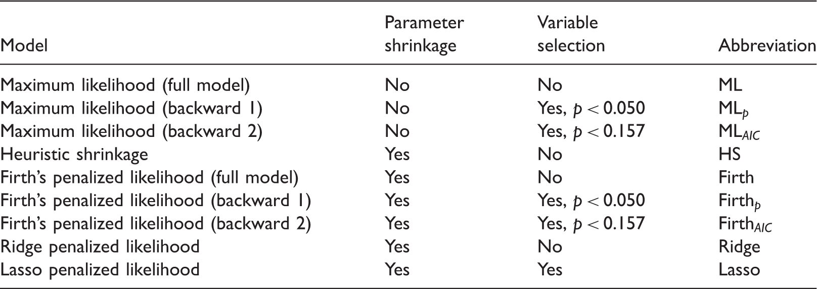
Our work is motivated by the lack of sample size guidance and uncertainty about the factors driving the predictive performance of clinical prediction models that are developed using binary logistic regression. We report an extensive simulation study to evaluate out-of-sample predictive performance (hereafter shortened to predictive performance) of developed prediction models, applying several methods for model development. We examine the predictive performance of logistic regression-based prediction models developed using conventional Maximum Likelihood (ML), Ridge regression, 23 Least absolute shrinkage and selection operator (Lasso), 24 Firth’s correction 25 and heuristic shrinkage after ML estimation. 26 Backwards elimination predictor selection using the conventional p = .05 and p = .157 (=AIC) stopping rules is also evaluated. Using a full-factorial approach, we varied EPV, the events fraction, number of candidate predictors, area under the ROC curve (model discrimination), distribution of predictor variables and type of predictor variable effects. The simulation results are summarized using metamodels.27,28
This paper is structured as follows. In section 2 we present models and notation. The design of the simulation study is presented in section 3, and the results are described in section 4. A discussion of our findings and its implications for sample size considerations for logistic regression is presented in section 5.
2 Developing a prediction model using logistic regression
2.1 General notation
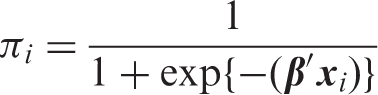
We define a logistic regression model for estimating the probability of an event occurring (Y = 1) versus not occurring (Y = 0) given values of (a subset of) P candidate predictors,
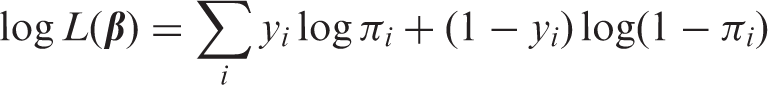
2.2 Maximum likelihood estimation and known finite sample properties
Conventionally, the
While ML logistic regression remains a popular approach to developing prediction models, ML is also known to possess several finite sample properties that can cause problems when applying the technique in small or sparse data. These properties can be classified into the following five separate and not mutually exclusive issues:
Issue 1: ML estimators are not optimal for making model predictions of the expected probability (risk) in new individuals. In most circumstances shrinkage estimators can be defined that have lower expected error for estimating probabilities in new individuals than ML estimators.30,31 The benefits of the shrinkage estimators over the corresponding ML estimators decreases with increasing EPV.
9
Issue 2: the predictor effects are finite sample biased.32,33 The regression coefficients from ML logistic regression models estimate the (multivariable) log-odds ratios for the individual predictors, which are biased towards more extreme effects, i.e. creating optimistic estimates of predictor effects for individual predictors in smaller data sets. This bias reduces with increasing EPV,34–36 but may not completely disappear even in large samples.
19
Issue 3: model estimation becomes instable when predictor effects are large or sparse (i.e. separation).37,38 The estimated predictor effects tend to become infinitely large in value when a linear combination of predictors can be defined that perfectly discriminates between events and non-events. Extreme probability estimates close to their natural boundaries of 0 or 1 is an undesirable consequence. Separation becomes less likely with increasing EPV.
19
Issue 4: model estimation becomes instable when predictors are strongly correlated (i.e. collinearity).9,39 If correlations between predictors are very strong, the standard errors for the predictor effects become inflated reflecting uncertainty about the effect of the individual predictor, although this has limited effect on the predictive performance of the entire model.
8
With increasing EPV, spurious predictor collinearity becomes less likely. Issue 5: commonly used automated predictor selection strategies (e.g. stepwise selection using p-values to decide on predictor inclusion
40
) cause distortions when applied in smaller data sets. In small datasets, predictor selection is known to: (i) lead to unstable models where small changes in the number of individuals – deletion or addition of individuals – can result in different predictors being selected7,8,41,42; (ii) cause bias in the predictor effects towards extremer values10,11; and (iii) reduce a model’s predictive performance when applied in new individuals, due to omission of important predictors (underfitting) or inclusion of many unimportant predictors (overfitting).9,11 The distortions due to predictor selection typically decrease with increasing EPV.
As these small and sparse data effects can affect the performance of a developed ML prediction model, and thus impact the required sample size for prediction model development studies, we additionally focus on four commonly applied shrinkage estimators for logistic regression. Each of these methods aims to reduce at least one of the aforementioned issues.
2.3 Regression shrinkage
2.3.1 Heuristic shrinkage logistic regression
Van Houwelingen and Le Cessie
43
proposed a heuristic shrinkage (HS) factor to be applied uniformly on all the predictor effects. The shrinkage factor is calculated as

The HS estimator was developed to improve a model’s predictive performance over the ML estimator in smaller data sets (issue 1).
43
However, in cases of weak predictor effects the HS estimator can perform poorly, as can be seen from equation (1) that
2.3.2 Firth logistic regression
Firth’s penalized likelihood logistic regression model25,38,45 penalizes the model likelihood by

The Firth estimator was initially developed to remove the first-order finite sample bias (issue 2) in ML estimators of logistic regression coefficients and other exponential models with canonical links.
25
As a consequence of its penalty function, the regression coefficients remain finite in situations of separation (issue 3).
38
More recently, Puhr and colleagues
21
evaluated the Firth’s estimator for improving predictive performance (issue 1), warning that it introduced bias in predicted probabilities toward
2.3.3 Ridge logistic regression
Ridge regression penalizes the likelihood proportionally to the sum of squared predictor effects:
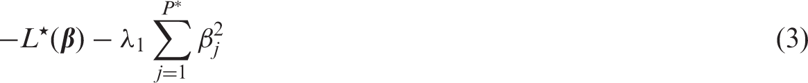


The Ridge estimator was originally developed to deal with collinearity (issue 4).23,39 Due to its penalty function it can also deal with separation (issue 3). Moreover, the Ridge estimator has been shown to improve predictive performance in smaller data sets that do not suffer from collinearity or separation (issue 1), although in some circumstances it showed signs of underfitting.15,48
2.3.4 Least absolute shrinkage and selection operator (Lasso) regression
Lasso regression penalizes the likelihood proportional to the sum of the absolute value of predictor effects:
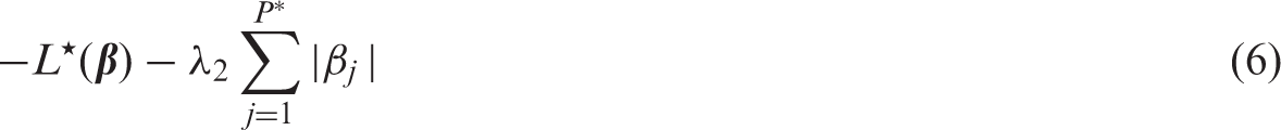
Lasso regression is attractive for developing prediction models as it simultaneously performs regression shrinkage (addressing issue 1) and predictor selection (by shrinking some coefficients to zero), while avoiding some of the adverse effects of regular automated predictor selection strategies (issue 5). It is also suited to handle separation (issue 3), but in the context of highly correlated predictors (issue 4), the Lasso has been reported to perform less well.15,49
3 Methods
This simulation study was set up to evaluate the predictive performance of various prediction modeling strategies in relation to characteristics of the development data. Our primary interest was in the size of the development data set relative to other data characteristics, such as the number of candidate predictors and the events fraction (i.e. Pr(Y = 1)). The various modeling strategies we considered are described in section 3 3.1, and the variations in data characteristics are described in section 3.2. A description of the predictive performance metrics and metamodels are given in sections 3.3.1 and 3.3.2, respectively. Software and error handling are given in section 3.4.
3.1 Modeling strategies
The predictive performance of the various logistic regression models as described in section 2 were evaluated on large sample validation data sets. These regressions correspond to different ways of applying regression shrinkage (ML regression applies none). For future reference, we collectively call these approaches “regression shrinkage strategies”.
We also evaluated predictive performance after backward elimination predictor selection. 40 This procedure starts by estimating a model with all P candidate predictor variables and considering the p-values associated with the predictor effects. For some pre-specified threshold value, the variable with the highest p-value exceeding the threshold value is dropped. The model is then re-estimated without the omitted variable. This process is continued until all the p-values associated with the effects of the predictors in the model are below the threshold. In this paper, we consider two commonly used threshold p-values values for ML and Firth’s regressions. We use conventional threshold p = 0.050 and a more conservative threshold p = 0.157. The latter is equivalent to the AIC criterion for selection of predictors. We collectively call the backwards elimination predictor selection approaches and Lasso (which performs predictor selection by means of shrinkage) “predictor selection strategies”.
3.2 Design and procedure
Design factorial simulation study (
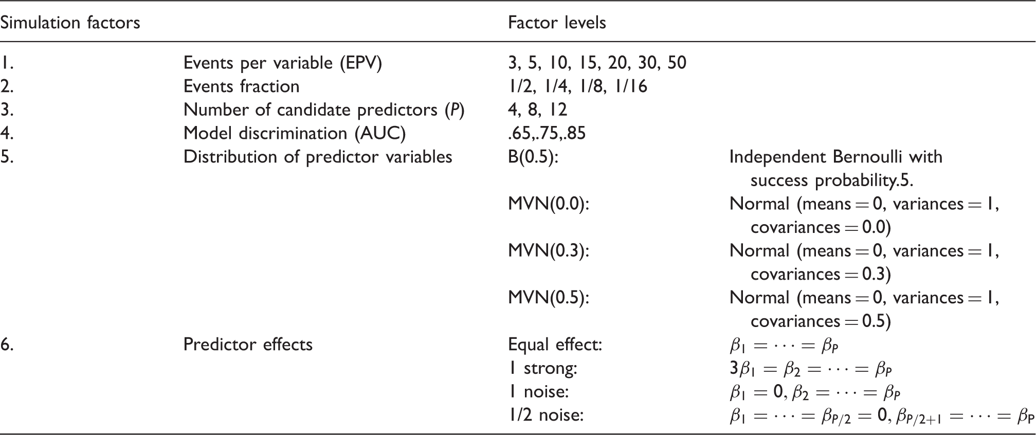
In total, 4032 unique simulation scenarios were investigated. For each of these scenarios, 5000 simulation runs were executed using the following steps:
A development data set was generated satisfying the simulation conditions (Table 1). For each of Nine binary logistic prediction models with different regression shrinkage and predictor selection strategies were estimated on the development data generated at step 1. These approaches are described in Table 2. A large validation data set was generated with sample size, The performance of the prediction models developed in step 2 is evaluated on the validation data generated in step 3. The measures of performance are detailed in section 3.3. Prediction models: parameter shrinkage and variable selection strategies.
More details about the development of the simulation scenarios appear in Web Appendix A.
3.3 Simulation outcomes
3.3.1 Predictive performance metrics
Model discrimination was evaluated by the average (taken over all validation simulation samples) loss in the area under the ROC-curve (ΔAUC). ΔAUC was defined by the average difference between the AUCs estimated on the generated data and the AUC of the data generating model (the AUC defined by simulation factor number 5, Table 1). ΔAUCs were expected to be negative, with higher values (closer to zero) indicating better discriminative performance.
Model calibration performance was evaluated by the median of calibration slopes (CS) and average calibration in the large (CIL). CS values closer to 1 and CIL closer to 0 indicate better performance. CS was estimated using standard procedures.52–54 Due to the expected skewness of slope distributions for smaller sized development data sets, medians rather than means and interquartile ranges rather than standard deviations were calculated. CS < 1 indicates model overfitting, CS > 1 indicates underfitting. CIL was calculated by average differences between the generated events fraction
The prediction error was evaluated by the average of Brier scores
55
(Brier), the square root of the mean squared prediction error (rMPSE) and mean absolute prediction error (MAPE). The rMPSE and MAPE are based on the distance between the estimated probabilities (
3.3.2 Metamodels
Variation in simulation results across simulation conditions was studied by using metamodels.27,28 The metamodels were used to quantify the relative impact of the various development data characteristics (taken as covariates in the metamodels) on a particular predictive performance simulation outcome (the outcome variable in the metamodel).
We considered the following covariates in the metamodel: development sample size (N), events fraction (
To facilitate interpretation, three separate metamodels were considered: i) a full model with all metamodel covariates, ii) a simplified model with only the development data size, events fraction and the number of candidate predictors, and for comparison: iii) a model with only development data EPV as a covariate. Metamodel ii was conceptualized before the start of the simulation study based on the notion that it would incorporate the same type of information as needed for estimating EPV before data collection, that is information available at the design phase of a prediction model development study (i.e. before the actual number of events are known).
The metamodels were estimated using linear regression with a Ridge penalty (i.e. Gaussian Ridge regression) specifying only linear main effects of the metamodel covariates. While more complex models (e.g. for interactions and non-linear effects) are possible, we found that linear main effects to be sufficient for constructing the metamodels. The Ridge metamodel tuning parameter was chosen based on 10-fold cross-validation that minimized mean squared error.
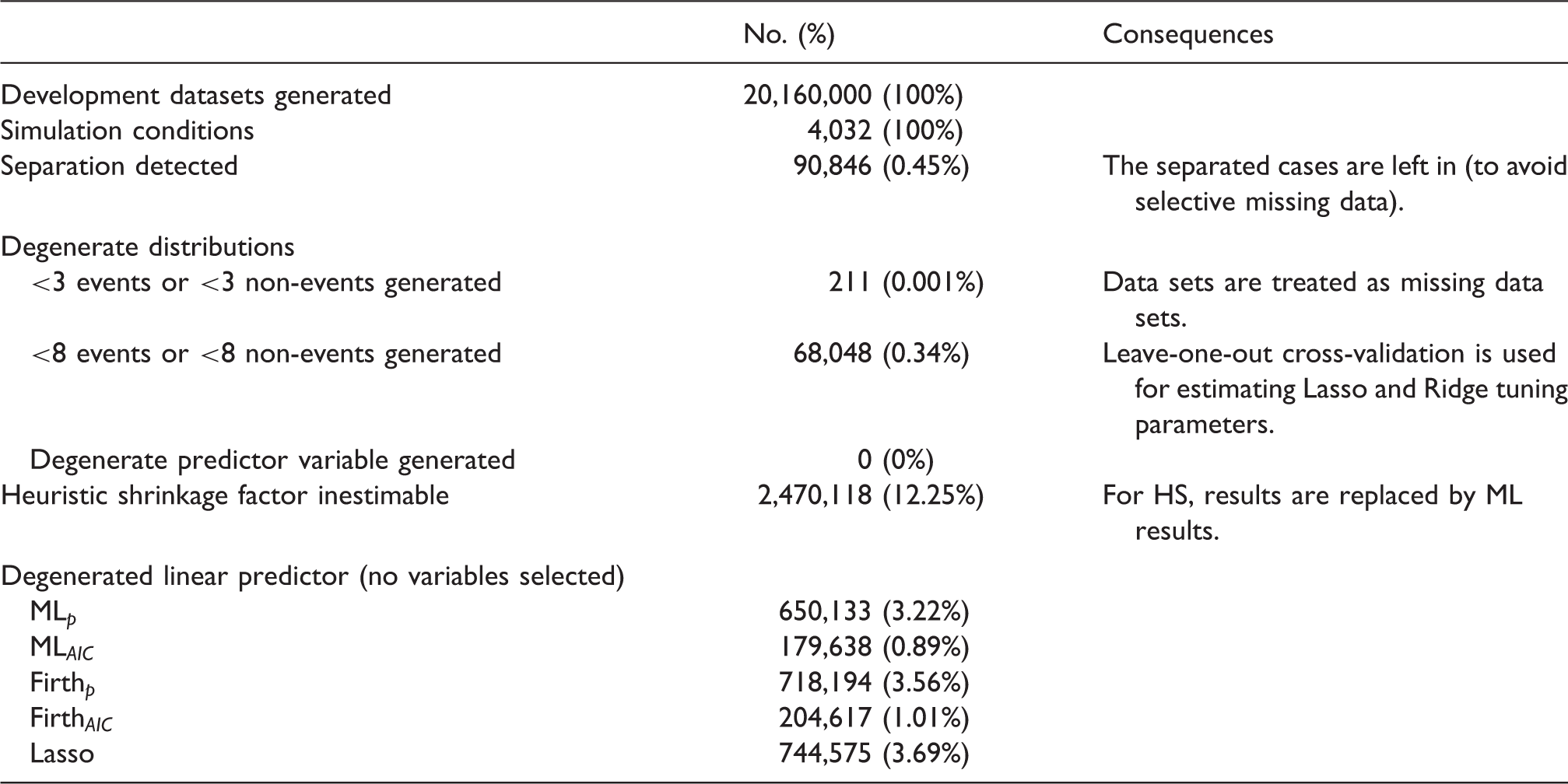
3.4 Software and estimation error handling
Simulation estimation errors and consequences.
4 Results
4.1 Predictive performance by relative size of development data
Figure 1 shows the average predictive performance of the various prediction models as a function of EPV and the events fraction. The impact of EPV and events fraction was consistent across the prediction models. There was improved predictive performance (i.e. reduction in average value for rMSPE and MAPE; ΔAUC closer to zero) when EPV increased (while keeping events fraction constant), and when the events fraction decreased (while keeping EPV constant). Differences between events fraction conditions decreased when EPV increased. Brier consistently improved (i.e. reduction in average value) with decreasing events fractions across prediction models, but showed little association with EPV beyond an EPV of 20.
Marginal out-of-sample predictive performance.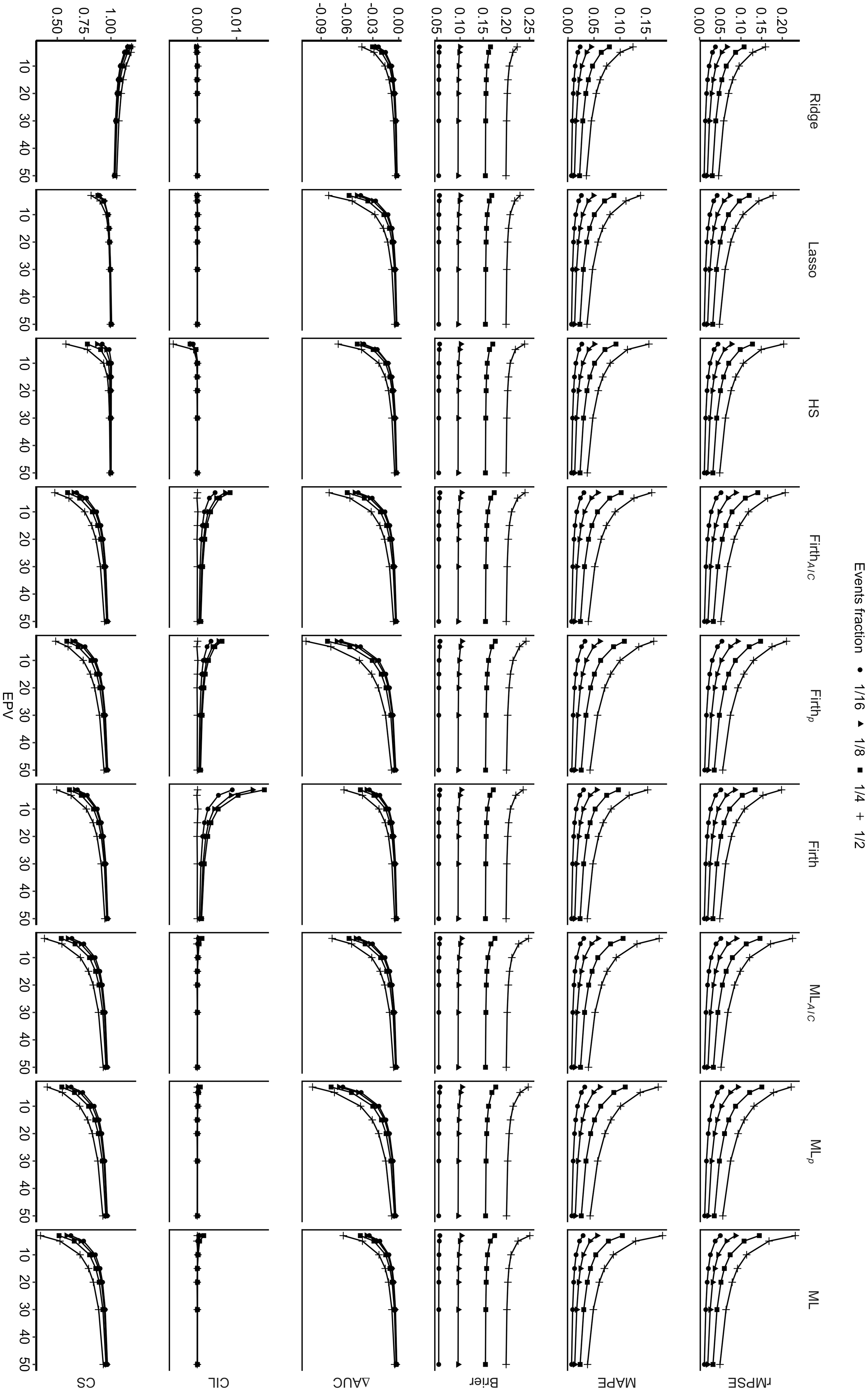
Close to perfect average values (a value of 0) were observed for CIL for all models across all studied conditions (Figure 1), except for the Firth regressions with and without predictor selection (Figure 1). This miscalibration-in-the-large occurred in lower EPV settings, and did not occur in the conditions where the events fraction was 1/2. CS improved (i.e. average values closer to 1) with increasing EPV and decreasing events fraction for all models. On average, all models except the Ridge regression showed signs of overfitting (CS values below 1). The Ridge regression consistently showed signs of underfitting (CS values above 1). For all models, improved CS values were observed when EPV increased (while keeping the events fraction constant) and the events fraction decreased (while keeping EPV constant).
4.1.1 Performance of regression shrinkage strategies by relative size of development data
Unsurprisingly, the impact of shrinkage lessened with increasing EPV as depicted in Figure 2. The active regression shrinkage strategies (Ridge, Lasso, HS, Firth) showed lower median rMPSE and MAPE values than the non-shrunken ML regression at EPV = 5 and EPV = 10. In those settings, Ridge, Lasso and HS regression showed more variability between simulation scenarios than Firth and ML. For simulation scenarios at EPV = 50, the differences between shrinkage strategies were smaller.
Boxplot distribution of out-of-sample predictive performance outcomes (restricted to conditions with events fraction = 1/2).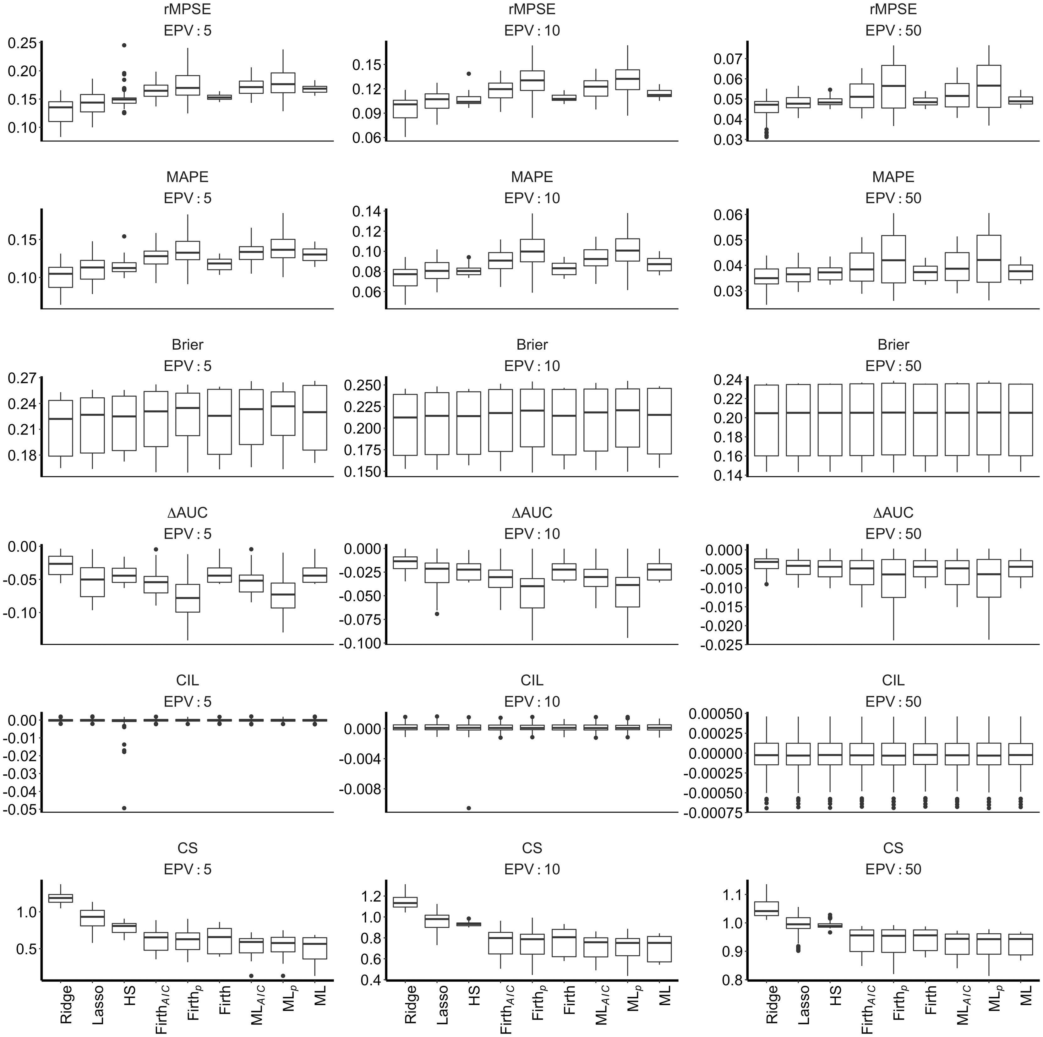
In Figure 2, Brier and CIL outcomes showed little variation between shrinkage strategies. Notice that for this figure the events fraction was kept constant at 1/2, miscalibration-in-the-large was therefore not observed for the Firth regression. Poor CIL and rMPSE for the HS model was observed in some conditions with a high rate of separation (results not shown). Only the Ridge regression showed superior performance on the outcome ΔAUC, with little differences between HS, Firth and ML, and slightly less favorable and more variable performance of the Lasso regression at EPV = 5 and EPV = 10. The Lasso regression yielded CS closest to optimal (value of 1).
4.1.2 Performance of predictor selection strategies by relative size of development data
Backwards elimination (ML p , ML AIC , Firth p and Firth AIC ) produced higher median rMPSE and MAPE than ML and Firth regressions that did not perform predictor selection (Figure 2). Median rMPSE and MAPE were more favorable for ML AIC and Firth AIC than ML p and Firth p . Backwards elimination also showed more variable MAPE and rMPSE values across the different simulation scenarios. The patterns were noticeable for the EPV = 5 and EPV = 10 conditions but did not completely disappear even at EPV = 50. Lasso regression had lower MAPE and rMPSE than the backwards elimination strategies and less variable results between conditions for the whole considered range of EPV.
Brier and CIL showed little variation between predictor selection strategies (Figure 2). For the predictor selection strategies, median ΔAUC were least favorable and more variable for Firth p and ML p , followed by ML AIC and Firth AIC , followed by Lasso. Lasso also yielded closer to optimal CS, with little differences observed between the backwards elimination strategies. These patterns were observed consistently across the considered EPV range.
4.2 Predictive performance by other development data characteristics
Figure 3 describes the average performances of prediction models. We left out Brier (only noticeable changes occurred when varying the AUC of the data generating mechanism) and CIL (close to optimal for all but Firth regressions) for this presentation.
Average relative out-of-sample performances of modeling strategies per simulation factor level.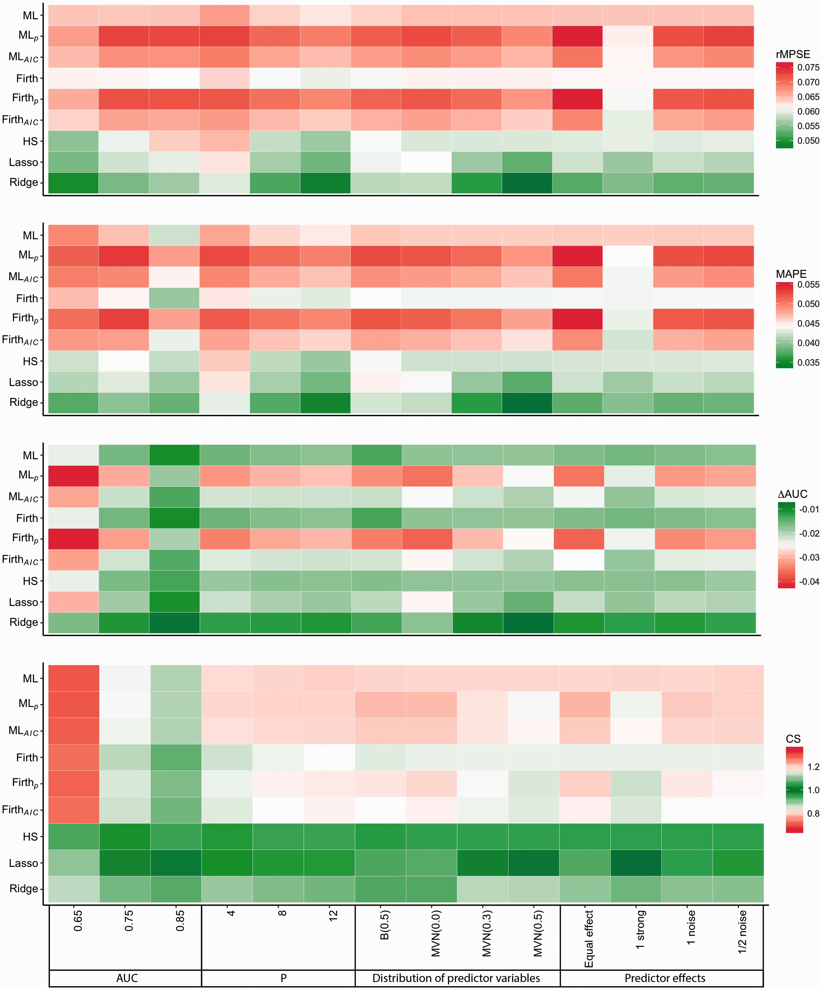
Lower AUC of the data generating mechanism was associated with poorer CS and ΔAUC outcomes. In conditions with AUC = 0.65, Ridge regression was superior in terms of rMPSE, MAPE and ΔAUC, while HS was superior in terms of CS. We also observed improved predictive performance as the number of predictors increased. This is partly due to a doubling of the development data size in our simulations when going from 4 to 8 predictors and three-fold increase in sample size when going from 4 to 12 predictors, a direct consequence of EPV as one of the chosen simulation factors.
With respect to the individual effects of the predictor variables (Figure 3), the average predictive performance of the variable selection strategies was best in conditions with one strong predictor. Effects of noise variables on the performances were negligible. Higher pairwise correlations between the predictors improved rMPSE, MAPE and ΔAUC for Ridge and Lasso and CS for Lasso. Higher correlations also increased the signs of underfitting of the Ridge regression (CS > 1).
4.3 Metamodels results
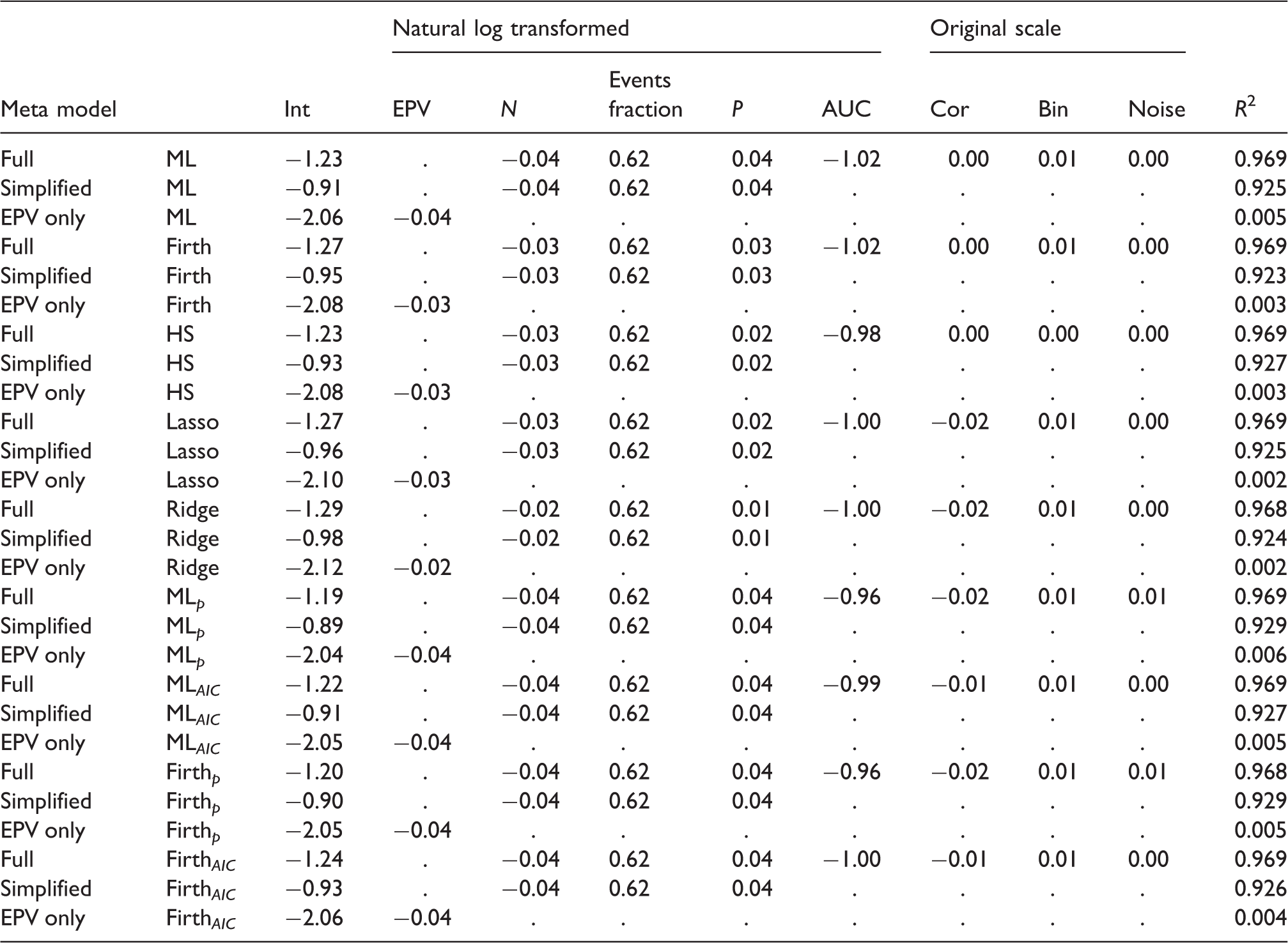
Results of simulation meta models: Outcome: ln(MSPE).
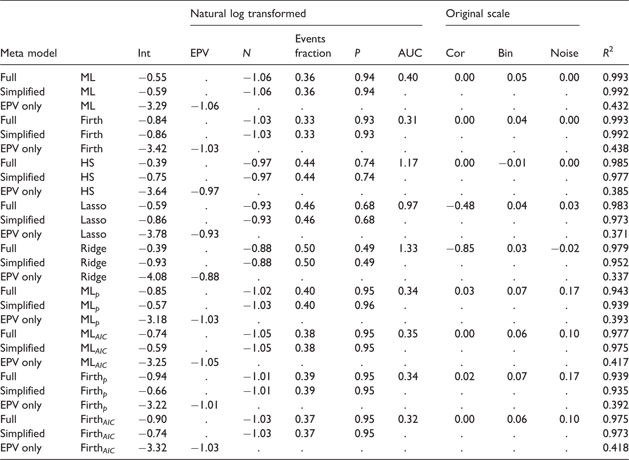
Full: metamodel with all eight meta-model covariates; Simplified: model with covariates N, events fraction and P, EPV only: meta model with EPV as a covariate. Int: Intercept; EPV: Events per variable; N: Sample size; P: number of candidate predictors; AUC: Area under the ROC-curve; Cor: Predictor pairwise correlations.
Results of simulation meta models: Outcome: ln(MAPE).
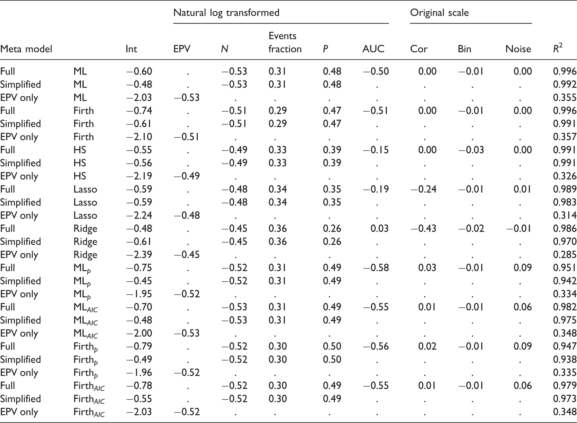
Full: metamodel with all eight meta-model covariates; Simplified: model with covariates N, events fraction and P, EPV only: meta model with EPV as a covariate. Int: Intercept; EPV: Events per variable; N: Sample size; P: number of candidate predictors; AUC: Area under the ROC-curve; Cor: Predictor pairwise correlations.
Results of simulation meta models: Outcome: ln(Brier).
Full: metamodel with all eight meta-model covariates; Simplified: model with covariates N, events fraction and P, EPV only: meta model with EPV as a covariate. Int: Intercept; EPV: Events per variable; N: Sample size; P: number of candidate predictors; AUC: Area under the ROC-curve; Cor: Predictor pairwise correlations.
Results of simulation meta models: Outcome: ΔAUC × 100.
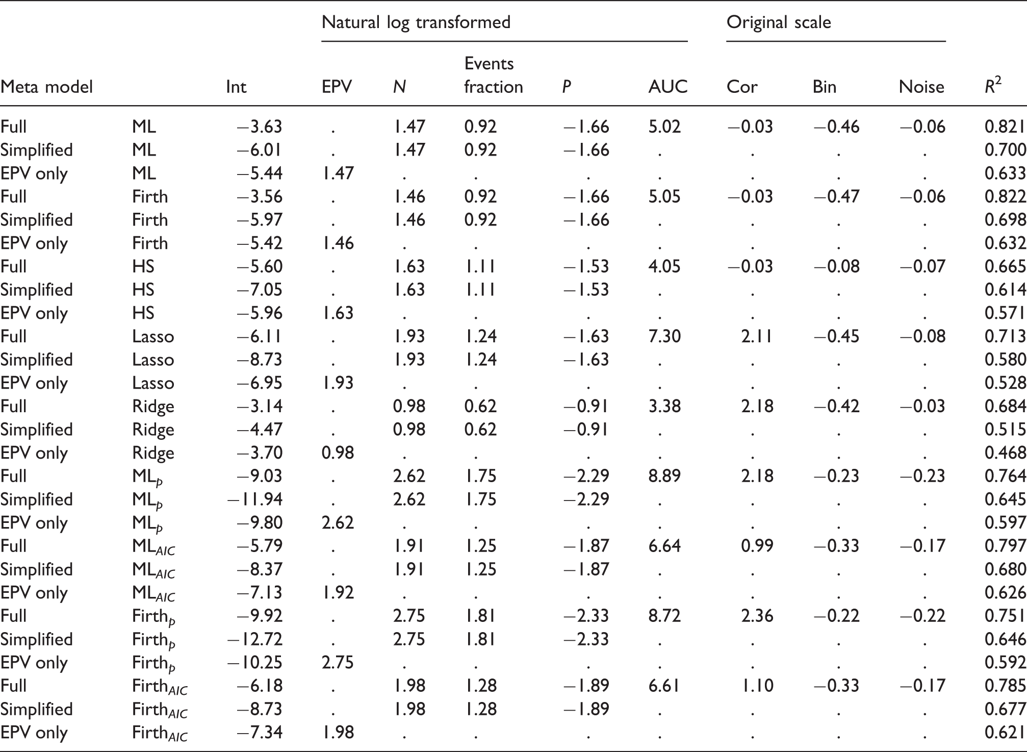
Full: metamodel with all eight meta-model covariates; Simplified: model with covariates N, events fraction and P, EPV only: meta model with EPV as a covariate. Int: Intercept; EPV: Events per variable; N: Sample size; P: number of candidate predictors; AUC: Area under the ROC-curve; Cor: Predictor pairwise correlations.
Results of simulation meta models: Outcome: CS.
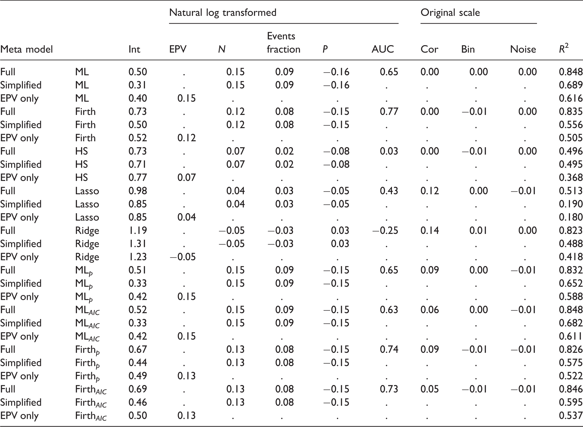
Full: metamodel with all eight meta-model covariates; Simplified: model with covariates N, events fraction and P, EPV only: meta model with EPV as a covariate. Int: Intercept; EPV: Events per variable; N: Sample size; P: number of candidate predictors; AUC: Area under the ROC-curve; Cor: Predictor pairwise correlations.
5 Discussion
This paper has investigated the impact of EPV and other development data characteristics in relation to modelling strategies on the (out-of-sample) predictive performance of prediction models developed with logistic regression. We showed that the EPV fails to have a strong relation with metrics of predictive performance across modelling strategies. Given our findings, it is clear that EPV is not an appropriate sample size criterion for binary prediction model development studies. Below we discuss our simulation results, followed by a discussion of the implications for sample size determination for prediction model development. A new strategy for such sample size consideration is proposed.
5.1 Simulation findings
Our study confirms previous findings that predictive performance can be poor for prediction models developed using conventional maximum likelihood binary logistic regression in data with a small number of subjects relative to the number of predictors. As expected, predictive performance generally improved when regression shrinkage strategies were applied, while backwards elimination predictor selection strategies generally worsened the predictive accuracy of the prediction model. These tendencies were observed consistently for discrimination (ΔAUC), calibration slopes (CS) and prediction error (rMPSE, MAPE, and Brier) outcomes. Calibration in the large was near ideal for all models in all simulation settings, except for Firth regression that showed upward biased estimation of probability towards
With larger sample sizes, the benefits (in terms of predictive performance) of the regression shrinkage strategies gradually declined, but predictive performance after shrinkage remained slightly superior or equivalent to ML regression even for larger sample sizes. Between the regression shrinkage strategies, the Ridge regression showed best discrimination (lowest average ΔAUC) and lowest prediction error (lowest average rMSPE, MAPE and Brier) performance when compared to Firth, Lasso and HS. Median CS of the HS and Lasso regression were closer to optimal than the Ridge regression, the latter showing signs of underfitting. The observed tendency to underfitting of Ridge regression is consistent with other recent simulation studies.16,48 In smaller samples, backwards elimination with conventional p = 0.050 and AIC criteria, generally performed worse than an equivalent regression without predictor selection or Lasso, even when only half of the predictor variables were randomly associated to the outcome. For conditions with EPV as large as 50, backwards elimination was found to yield higher rMSPE and MAPE than the equivalent model with all variables left in. Between the backward elimination criteria, the more conservative AIC criterion was found to produce better average predictive performance than p = 0.050, in accordance with earlier work.9,11
The metamodels fitted on the simulation results revealed that between simulation variation of (r)MPSE, MAPE and Brier could largely be explained by a linear model with three covariates: sample size, the events fraction and the number of candidate predictors. The joint effect of these three covariates on prediction error tended to become slightly weaker when regression shrinkage or variable selection strategies were applied. ΔAUC and CS were found to be more unpredictable by the metamodel regression. ΔAUC and CS were found to be particularly sensitive to the prediction model development strategy employed (e.g. whether regression shrinkage or predictor selection was used) and, importantly, dependent on the AUC of the data generating mechanism.
Some limitations apply to our study. The broad setup of our simulations, with over 4000 unique scenarios, does allow for a generalization of the findings to a large variety of prediction modeling settings. However, as with any simulation study, the number of investigated scenarios was finite and extrapolation of our findings far beyond the investigated regions is not advised. A total of nine prediction modeling strategies were investigated. In practice, we expect that other approaches to regression shrinkage and predictor selection than we considered may sometimes be preferable (e.g. Elastic Net, 49 non-negative Garrotte, 60 random forest 61 ). Finding optimal strategies for developing clinical prediction models in small or sparse data was not the main objective of the current study but is a worthwhile topic for future research.
5.2 Implications for sample size considerations
There is general consensus on the importance of having data of adequately size when developing a prediction model. 2 However, consensus is lacking on the criteria to determine what size would count as adequate.
Our results showed that the recommended minimal EPV criteria for prediction model development, notably the EPV Relation required sample size and events fraction. Calculations based on metamodels with criterion values that were kept constant. For illustration purposes, the criterion values were chosen such that they would intersect at events fraction = 1/2.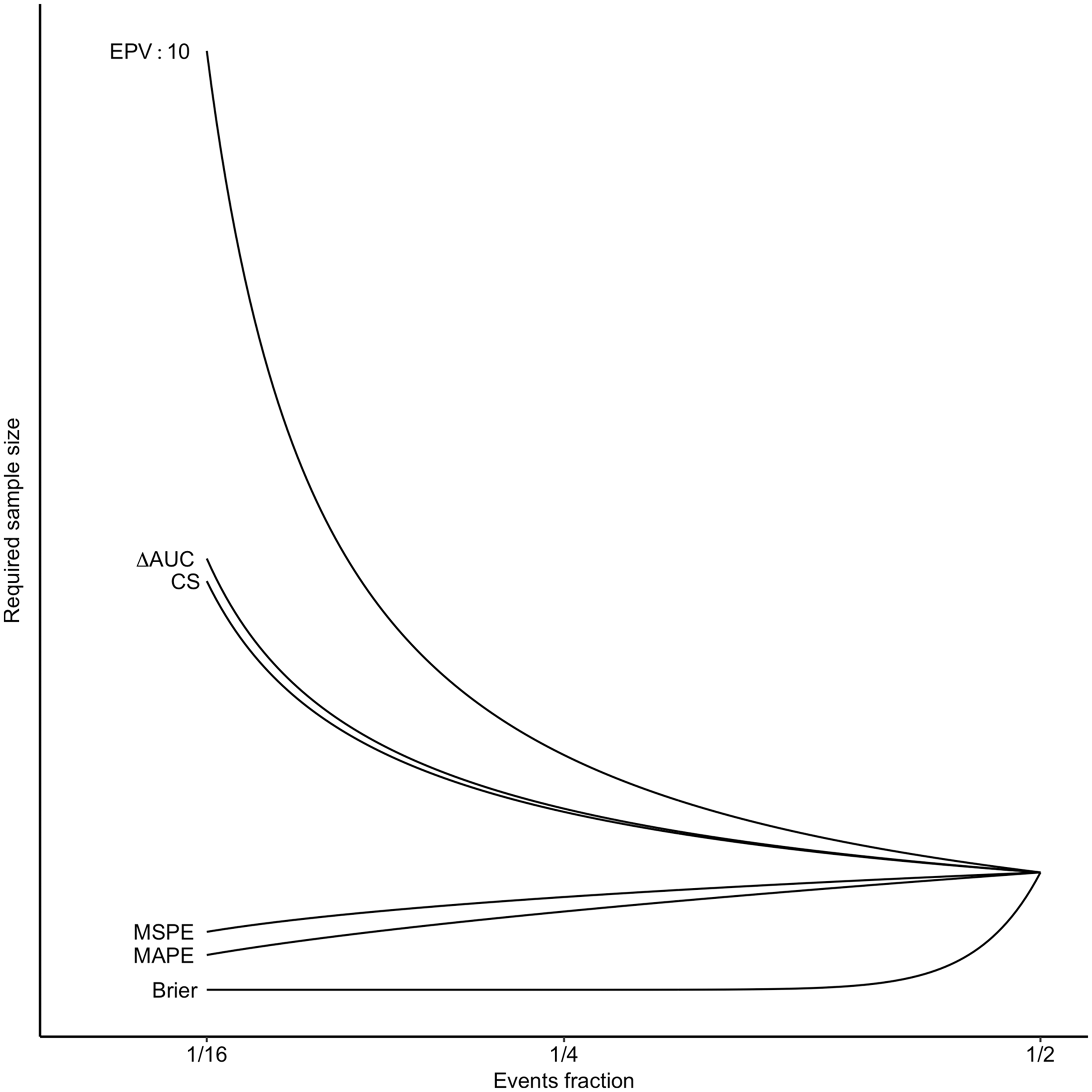
The search for new minimal sample size criteria inherently calls for abandoning EPV as the sole sample size criterion. Alternatives for sample size must have a predictable relationship with future predictive performance and be on a scale that is interpretable for users. It is our view that general single threshold values should be avoided. Instead, sample size determination should be based on threshold values on an interpretable scale that ensure predictive performance that is fit for purpose. What counts as fit for purpose varies from application to application (e.g. clinical prediction models for informing short-term high-risk treatment decisions may differ from the requirements for long-term low-risk decisions). It is the duty of the researcher to define what constitutes as fit for purpose in context and explain how the sample size was arrived at (see also: the TRIPOD statement2,3).
5.3 New sample size criteria
Out-of-sample (r)MSPE and MAPE are natural metrics to determine sample size adequacy of prediction models, as they define the expected distance (squared or absolute) for new individuals between the estimated probabilities for new patients and their unobservable “true” values. Because clinical prediction models are primary used to estimate probabilities for new individuals,3–5 rMSPE and MAPE have direct relevance when developing a prediction model.
The out-of-sample rMPSE and MAPE can be approximated via simulations as we have done in this paper. Our simulation code is available via GitHub (https://github.com/MvanSmeden/Beyond-EPV). Alternatively, rMSPE and MAPE may be approximated via the results of our metamodels (Table 4). For instance, at a sample size of N = 400, with P = 8 candidate predictors and an expected event fraction of 1/4, the predicted out-of-sample rMPSE is 0.065 when ML model (without variable selection) is applied and 0.053 for Ridge regression; MAPE is 0.045 for the ML model and 0.038 for the Ridge regression. Obviously, whether or not these expected “average” prediction errors on the probability scale are acceptable or not depends on the intended use of the prediction model (i.e. N = 400 may not be sufficient for accurate estimation of probability for high risk treatment decisions, even though for this example EPV = 20).
We warn readers that these out-of-sample performance predictions from the simulation metamodels have not been externally validated and that approximations may not work well far outside the range of investigated simulation settings. In particular, using these approximations for sample size calculations with very low events fractions may yield unacceptably poor discrimination and calibration performances (see Figure 4).
6 Conclusion
The currently recommended sample size criteria for developing prediction models, notably the EPV
Supplemental Material
Supplemental material for Sample size for binary logistic prediction models: Beyond events per variable criteria
Supplemental Material for Sample size for binary logistic prediction models: Beyond events per variable criteria by Maarten van Smeden, Karel GM Moons, Joris AH de Groot, Gary S Collins, Douglas G Altman, Marinus JC Eijkemans and Johannes B Reitsma in Statistical Methods in Medical Research
Footnotes
Acknowledgement
We thank Prof Dr Richard D Riley for his constructive comments on an earlier version of this manuscript.
Declaration of conflicting interests
The author(s) declared no potential conflicts of interest with respect to the research, authorship, and/or publication of this article.
Funding
The author(s) disclosed receipt of the following financial support for the research, authorship, and/or publication of this article: This work was supported by the Netherlands Organisation for Scientific Research (project 918.10.615).
References
Supplementary Material
Please find the following supplemental material available below.
For Open Access articles published under a Creative Commons License, all supplemental material carries the same license as the article it is associated with.
For non-Open Access articles published, all supplemental material carries a non-exclusive license, and permission requests for re-use of supplemental material or any part of supplemental material shall be sent directly to the copyright owner as specified in the copyright notice associated with the article.