Sage Journals: Discover world-class research

Abstract

In several areas of clinical research, it is common for trials to assign different sites of the participants’ bodies to different interventions. For example, a randomized controlled trial comparing surgical techniques for correcting myopia may randomize each eye of a participant to a different operation. Under such bilateral (‘split-body’) interventions, the observations from each participant are correlated. It is challenging to account for these correlations at the meta-analysis level, especially when the outcome is rare. Here, we present a meta-analysis model based on the bivariate binomial distribution. Our model can synthesize studies on patients who received one intervention at one body site, patients who received two interventions at different sites or a mixture of these two groups. The model can analyse studies with zero events in one or both treatment arms and can handle the case of incomplete data reporting. We use simulations to assess the performance of our model and to compare it with the bivariate beta-binomial model. In the case of bilateral interventions, our model performed well and outperformed the bivariate beta-binomial model in all scenarios explored. We illustrate our methods using two previously published meta-analyses from the fields of orthopaedics and ophthalmology. We conclude that our model constitutes a useful new tool for the meta-analysis of binary outcomes in the presence of split-body interventions.

Keywords

1 Introduction

Correlated outcome data can occur in trials when multiple related outcomes are measured, when a single outcome is measured at multiple time-points or when patients receive more than one intervention. Typical examples of the latter category are the cross-over trials and the within-person randomized trials.¹ For example, outcomes from patients receiving different surgical operations for myopia in each of their eyes or different carpal-tunnel release methods in each of their arms are correlated. We will refer to this kind of interventions as ‘split-body’ or ‘bilateral’ interventions. At the meta-analysis level, disregarding the correlation induced by bilateral interventions and analysing observations as if they belong to different patients may affect the precision of the pooled estimates.^2–6

For the case of binary outcomes, if studies with bilateral interventions report the full, ‘cross-classified’ information (number of events by patients and treatments) one can readily account for the correlations. This cross-classified information is, however, usually unavailable to the meta-analysts. If not available, an assumed value of the correlation between the arm-specific effects (e.g. the log-odds) can be imputed and the data can be synthesized using a bivariate normal likelihood.

While this approach might be reasonable for efficacy outcomes, it is problematic for safety outcomes. Safety outcomes are often rare and in this case, the normal approximation performs poorly while the estimation of the between-study variance (heterogeneity) becomes challenging.⁷ Moreover, the normal approximation of the log-odds or log risks cannot be readily used in the presence of studies with zero events in one (‘single-zero’ studies) or both arms (‘double-zero’ studies). Such studies are frequently encountered in meta-analyses: in a sample of 500 Cochrane reviews, 30% included at least one single-zero, while 34% of these reviews included at least one meta-analysis with a double-zero study.^8,9 In such cases, researchers usually resort to performing a ‘continuity correction’ i.e. they add a factor in each cell of the corresponding two-by-two table. The choice of the factor, however, may heavily affect the meta-analysis estimates^10,11 and might lead to paradoxical results.¹² Double-zero studies are typically excluded from meta-analysis.⁸

Alternative meta-analysis models that do not require a continuity correction and do not exclude studies have been suggested. These include generalized linear mixed models,¹³ using the arcsine difference,¹⁴ a Poisson-Normal model,¹⁵ a zero-inflation model,¹⁶ a Poisson-Gamma model,¹⁷ Firth's logistic regression model¹⁸ and a bivariate beta-binomial model^19–21 (sometimes called Sarmanov beta-binomial model). Kuss⁸ reviewed and compared 10 different methods for meta-analysing rare events in a simulation study and recommended the use of the beta-binomial model for the meta-analysis of rare events. None of the aforementioned methods, however, can account for correlations induced by bilateral interventions.

Although there are methods available for meta-analysing correlated binary outcomes, it is not clear whether they are appropriate when the outcome is rare and when reporting is incomplete. In this paper, we propose a new model fitted within a Bayesian framework that can be used to meta-analyse studies of unilateral design (each patient received one intervention in one body part), bilateral design (all patients received two interventions in different body parts) or a mixed design (where some patients received one intervention and some patients both). Our model uses a bivariate binomial likelihood that explicitly accounts for the correlations induced by the presence of bilateral interventions without employing the normal approximation. Our model can accommodate a meta-analysis in the presence of rare events, without excluding single- or double-zero studies from the dataset and can handle the case of incomplete reporting in the original studies, i.e. when cross-classified information is not provided.

The paper is structured as follows. In section 2, we describe the datasets from orthopaedics and ophthalmology we use to exemplify our methods. We chose these particular examples because they include studies of different designs and they cover both the case of rare and common outcomes. In section 3, we present our model and discuss how it can be applied for the case of studies of different designs. In section 4, we present results from simulations that we conducted in order to assess the performance of our model and to compare it with the previously recommended beta-binomial model. In section 5, we present results from the examples. Finally, in section 6, we highlight our main findings, summarize the strengths and weaknesses of our approach and discuss possible extensions.

2 Example datasets

2.1 Two surgical treatments for carpal tunnel syndrome

Our first example comes from a Cochrane review²² that compared the endoscopic release vs. any other open surgical intervention for carpal tunnel syndrome (CTS). CTS is a painful compression of a nerve at the root of the hand. One of the safety outcomes was the occurrence of minor complications (such as numbness around the incision or superficial infection) reported in 24 studies. Minor complications were rare: five out of 24 studies were single-zero and four were double-zero. In section 1.1. of the online Appendix, we provide a detailed description of the data. We categorize the 24 studies in four different types, depending on their design and reporting:

Unilateral design (studies 1–12): patients received one intervention in one of their arms. Studies report number of patients and number of events per intervention group.

Bilateral design (studies 13–15): each patient received both interventions in different arms. In the CTS example, these studies reported number of patients and number of events per intervention group. They did not report cross-classified information (e.g. number of patients with events in both of their arms, with events in none of their arms, with events in one of their arms).

Mixed design (studies 16–22): some patients received one intervention in one of their arms, and some patients received both in different arms. In the CTS example, these studies reported the corresponding number of patients in each group (or we calculated them from the reported data). No cross-classified information was reported.

Unknown design (studies 23–24): these studies only report number of events and number of treated arms, per intervention group. They do not provide information on how many patients (if any) received both interventions in both of their arms.

2.2 Two surgical techniques for correcting myopia

Our second example comes from a Cochrane review for the comparison of laser-assisted in-situ keratomileusis versus photorefractive keratectomy for myopia.²³ The outcome of interest is the proportion of eyes with uncorrected visual acuity (UCVA) of 20/20 or better, at six months after treatment. Ten studies reported this outcome. Two studies had a unilateral design, five studies had a bilateral design and did not report any cross-classified information and three studies had an unknown design, i.e. they did not report the exact number of unilateral and bilateral interventions. We present the data for this example in section 1.2 of the online Appendix. Table 1 summarizes the type of data that were available for each example and introduces notation.

Table 1.

Summary of the type of data available for the CTS and myopia examples.^a

Design	Data provided in the studies	No. of studies available
Unilateral design: Only one body part per patient was treated	$r_{A}$ , $N_{A},$ $r_{B}$ , $N_{B}$ , $N = N_{A} + N_{B}$	CTS: 12
	$r_{A}$ , $N_{A},$ $r_{B}$ , $N_{B}$ , $N = N_{A} + N_{B}$	Myopia: 2
Bilateral design: Each patient received both interventions in different body parts	$r_{A}$ , $r_{B}$ , $N = N_{A} = N_{B}$	CTS: 3
	$r_{A}$ , $r_{B}$ , $N = N_{A} = N_{B}$	Myopia:5
Mixed design: Mixture of unilateral and bilateral interventions; some patients received one intervention in one body part, some received both interventions in different body parts	$r_{A}$ , $N_{A}$ , $r_{B}$ , $N_{B}$ , N $max (N_{A}, N_{B}) \leq N$ $N < N_{A} + N_{B}$	CTS: 7
		Myopia: 0
Unknown design: No information on whether any patients received both interventions	$r_{A}$ , $N_{A}$ $r_{B}$ , $N_{B}$	CTS: 2
	$r_{A}$ , $N_{A}$ $r_{B}$ , $N_{B}$	Myopia: 3

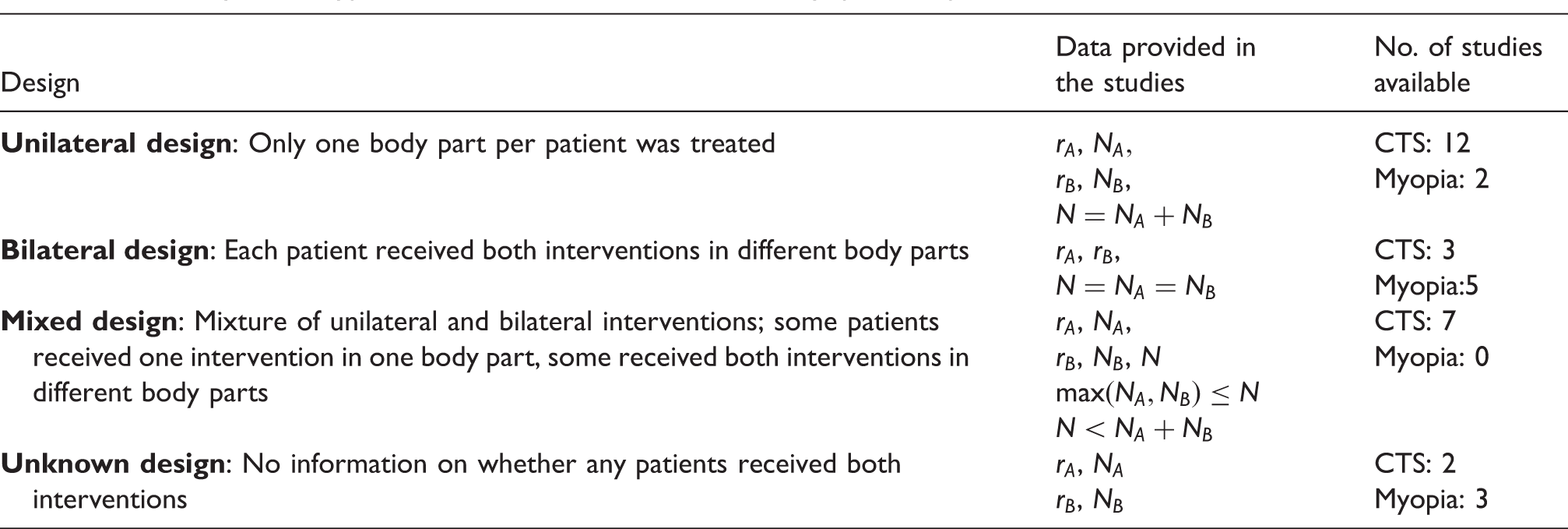
CTS: carpal tunnel syndrome.

r_A (r_B) denotes the number of events and N_A (N_B) the number of patients who received intervention A (B). With N, we denote the total number of patients included in each study.

3 Methods

In this section, we present our random effects meta-analysis model that can be fit within a Bayesian framework. Methods for estimating and summarizing treatment effects from studies of unilateral and bilateral design are established and we start by revising them. However, the number of events per patient and intervention (the cross-classified information) is required for a proper analysis of studies of bilateral design. Such information is often not available. We introduce a model that bypasses this problem, and then we extend it for the analysis of studies of mixed and unknown design. In section 3.6, we discuss approaches for formulating prior distributions for all model parameters. We only consider the case of a binary outcome, i.e. each patient can only have up to one event per intervention.

3.1 Unilateral design

Let's assume that a study i compared interventions A and B, and that it applied only unilateral interventions. Let us assume $N_{i, A}$ ( $N_{i, B}$ ) patients received intervention A (B), and that we observed $r_{i, A}$ ( $r_{i, B}$ ) events. Given that each patient only received one intervention, the events are independent and we can assume two univariate binomial distributions. The estimated probabilities of event in each intervention group of each study can be used to estimate study-specific intervention effects, with their corresponding standard errors. These study-specific estimates can be synthesized at a second stage, under a usual meta-analytical model. This corresponds to a two-stage meta-analysis model. The drawback of two-stage models is that in the second stage, the study-specific intervention effects are assumed to follow a normal distribution, and that the variances are assumed to be exactly known.²⁴ This implies that a two-step approach is generally suboptimal for the case of binomially distributed data, and even more so when the data are sparse.

Alternatively, we can do the meta-analysis in a single step using a hierarchical model. A one-step model can be written as follows

\begin{array}{l} r_{i, A} \sim B i n (p_{i, A}, N_{i, A}), r_{i, B} \sim B i n (p_{i, B}, N_{i, B}) \\ l o g i t (p_{i, A}) = u_{i} + \frac{θ_{i}}{2}, l o g i t (p_{i, B}) = u_{i} - \frac{θ_{i}}{2} \\ θ_{i} \sim N (μ, τ^{2}) \\ u_{i}, μ, τ \sim \dots (p r i o r d i s t r i b u t i o n s) \end{array}

(1)

where

θ_{i}

is the study-specific log-odds ratio (OR), μ is the summary log-OR and

τ^{2}

the heterogeneity variance.

u_{i}

is a nuisance parameter that corresponds to the log-odds of the mean event rate in both intervention groups (we will refer to this quantity as ‘average risk’ throughout this paper). For

u_{i}, μ

and τ prior distributions are required. An alternative, one-stage model can be formulated by assuming exchangeability on the average risk

\begin{array}{l} r_{i, A} \sim B i n (p_{i, A}, N_{i, A}), r_{i, B} \sim B i n (p_{i, B}, N_{i, B}) \\ l o g i t (p_{i, A}) = u_{i} + \frac{θ_{i}}{2}, l o g i t (p_{i, B}) = u_{i} - \frac{θ_{i}}{2} \\ u_{i} \sim N (μ_{u}, σ_{u}^{2}), θ_{i} \sim N (μ, τ^{2}) \\ μ_{u}, μ, τ, σ_{u} \sim \dots (p r i o r d i s t r i b u t i o n s) \end{array}

(2)

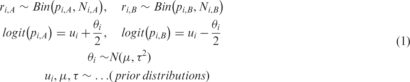
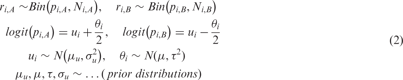
The advantage of model (equation (2)) is that in the case of rare events, it facilitates the estimation of the parameters by ‘borrowing strength’ for the average risk across studies. The price to pay is that the model makes an additional assumption, i.e. the exchangeability of average risk across studies. Note that one can write alternative one-stage models, e.g. by assigning a prior to $p_{i, A}$ or $p_{i, B}$ instead of $u_{i}$ . We discuss this assumption more in the Discussion.

3.2 Bilateral design: studies providing cross-classified information

Let us assume that study i compared interventions A and B and that each patient received both interventions. Let us also assume that the study reports the full cross-classified information, as shown in Table 2. For simplicity, in what follows, we drop the study index.

Table 2.

‘Contingency’ table for a study of bilateral design with N patients, providing the full cross-classified information.^a

	$B^{+}$	$B^{-}$	Total
$A^{+}$	$n_{1}$	$n_{2}$	$r_{A}$
$A^{-}$	$n_{3}$	$n_{4}$	$N - r_{A}$
Total	$r_{B}$	$N - r_{B}$	N

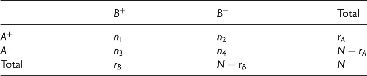
A⁺(A⁻) denotes events (non-events) in intervention A; likewise for treatment B. n₁ denotes the number of patients with events for both interventions. n₂ is the number of patients with an event for A and a non-event for B, the opposite is n₃. n₄ denotes the number of patients with no events in any intervention.

From this table, we can estimate the probability of an event in each treatment. E.g. by maximizing the likelihood, we estimate ${\hat{p}}_{A} = r_{A} / N$ , ${\hat{p}}_{B} = r_{B} / N$ , and also ${\hat{p}}_{k} = n_{k} / N$ , where $k = 1, 2, 3, 4$ . If we choose odds-ratio as an effect size, we have $\hat{l o g O R} = l o g i t ({\hat{p}}_{A}) - l o g i t ({\hat{p}}_{B})$ . Observations ( $r_{A}$ and $r_{B}$ ) belong to the same patients, which means that the estimates for the two probabilities ${\hat{p}}_{A}$ and ${\hat{p}}_{B}$ are correlated within each study. The estimated $\hat{v a r} (\hat{l o g O R})$ should thus include a covariance term

\hat{v a r} (\hat{l o g O R}) = \hat{v a r} (l o g i t ({\hat{p}}_{A})) + \hat{v a r} (l o g i t ({\hat{p}}_{B})) - 2 \hat{C o v} (l o g i t ({\hat{p}}_{A}), l o g i t ({\hat{p}}_{B}))

(3)

This covariance term can be written as a function of Pearson's ϕ coefficient,²⁵ which is a measure of the correlation between two binary variables of a 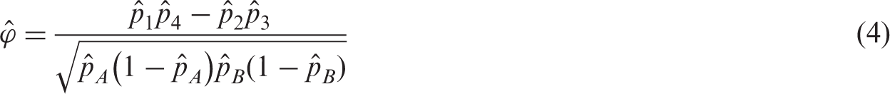$2 \times 2$ table²⁶

\hat{ϕ} = \frac{{\hat{p}}_{1} {\hat{p}}_{4} - {\hat{p}}_{2} {\hat{p}}_{3}}{\sqrt{{\hat{p}}_{A} (1 - {\hat{p}}_{A}) {\hat{p}}_{B} (1 - {\hat{p}}_{B})}}

(4)

If we ignore the cross-classifications ( $n_{1}$ , $n_{2}, n_{3}$ and $n_{4}$ ) and use only the margins of Table 2, we treat the two intervention groups as if they were independent. In that case, the variance of the effects will not account for any covariance. This, in turn, will lead to the precision of the estimated relative effects being either inflated or deflated, depending on the underlying correlation between $r_{A}$ and $r_{B}$ . In most clinical examples, we would expect a positive correlation, so ignoring this correlation is generally expected to lead to less precise results.

In order to correctly account for this covariance, we need to use the full information and to employ a multinomial likelihood

(n_{1}, n_{2}, n_{3}, n_{4}) \sim Multinomial (p_{1}, p_{2}, p_{3}, p_{4}; N)

(5)

We can then estimate ${\hat{p}}_{1}, {\hat{p}}_{2}, {\hat{p}}_{3}$ and ${\hat{p}}_{4}$ , and we can identify ${\hat{p}}_{A} = {\hat{p}}_{1} + {\hat{p}}_{2}$ and ${\hat{p}}_{B} = {\hat{p}}_{1} + {\hat{p}}_{3}$ and calculate their covariance. At the meta-analysis level, we can use model (equation (2)) with a multinomial instead of a binomial likelihood.

For this analysis, one would need to have the cross-classified information of Table 2. Alternatively, if the study has performed an appropriate analysis, one could use the reported results (e.g. standard error or p value) to reverse-engineer equation (3) so as to calculate the entries of Table 2 and then use the correct multinomial distribution of equation (5). To our experience, published studies rarely report the information needed for such back-calculations. To make matters worse, some of the studies may include a mixture of unilateral and bilateral interventions, often without reporting the corresponding numbers. In the following sections, we show how to correctly analyse the data in such circumstances. We start by the simplest cases of data availability and move on to more complex situations.

3.3 Bilateral design: studies that do not provide cross-classified information

Let us assume a bilateral study where only the margins of Table 2 are reported (i.e. $r_{A}, r_{B}$ and N). The exact likelihood of the marginal data (i.e. $r_{A}$ , $r_{B}$ and N) is given by Gonin and Aitken in the form of a bivariate binomial distribution.^27–29 More specifically, the probability of having $r_{A}$ events in intervention group A and $r_{B}$ events in B, in a total of N patients that received both interventions is given by

P (r_{A}, r_{B}) = Σ_{n_{1} = max (0, r_{A} + r_{B} - N)}^{min (r_{A}, r_{B})} \frac{N!}{n_{1}! (r_{A} - n_{1})! (r_{B} - n_{1})! (N - r_{A} - r_{B} + n_{1})!} \times p_{1}^{n_{1}} p_{2}^{r_{A} - n_{1}} p_{3}^{r_{B} - n_{1}} p_{4}^{N - r_{A} - r_{B} + n_{1}}

(6)

where

p_{1}

p_{2}

p_{3}

and

p_{4} = 1 - p_{1} - p_{2} - p_{3}

are the probabilities corresponding to each cell of Table 1.

Equation (6) runs through the total number of different set-ups of the contingency table that gives rise to the same margins $r_{A}$ and $r_{B}$ . One could in principle assume an uninformative prior for $p_{1}$ , $p_{2}$ , $p_{3}$ and $p_{4}$ (e.g. through a uniform Dirichlet distribution) and then use the likelihood of equation (6) to obtain the posterior distribution for these four probabilities. As discussed in the previous section, the estimation of the relative effects between the two interventions would use ${\hat{p}}_{A} = {\hat{p}}_{1} + {\hat{p}}_{2}$ and ${\hat{p}}_{B} = {\hat{p}}_{1} + {\hat{p}}_{3}$ . This would induce a correlation between the estimates of $p_{A}$ and $p_{B}$ .

However, this approach would result to an average of all possible values for this correlation. It might be the case, however, that having an event in A is highly correlated with having an event in B. This could happen when for instance events are induced by the presence of a certain characteristic in the patient, irrespective of intervention received. In the CTS example, it might be the case that patients with manual labour professions are more prone to having a minor complication in both arms. In such cases, there would be a strong underlying correlation, which would not show in this approach. A hypothetical example to clarify this point is presented in Figure 1, where a study of 100 bilateral interventions reports 60 events in intervention A and 70 in B, but no information on the cross-classification. The likelihood of equation (6) sums across all possible contingency tables: from those that correspond to a high correlation, like the one with $n_{1} = 60$ in Figure 1 ( $ϕ = 0.80)$ , up to those that correspond to a strong negative correlation like the bottom configuration in Figure 1 (where $ϕ = - 0.53)$ . I.e. equation (6) incorporates a correlation of $p_{A}$ and $p_{B}$ based on the average of all possible values of ϕ. Essentially, the estimates for $p_{A}$ and $p_{B}$ are correlated in a study of a bilateral design, but one cannot estimate this correlation using only the margins of the 2 × 2 table.

Figure 1.

Three possible configurations of the 2 × 2 table of a study of 100 bilateral interventions reporting only the margins of the contingency table. The first configuration corresponds to a large positive correlation (φ = 0.80), the second to no correlation (φ = 0), the third to a large negative correlation (φ = –0.53).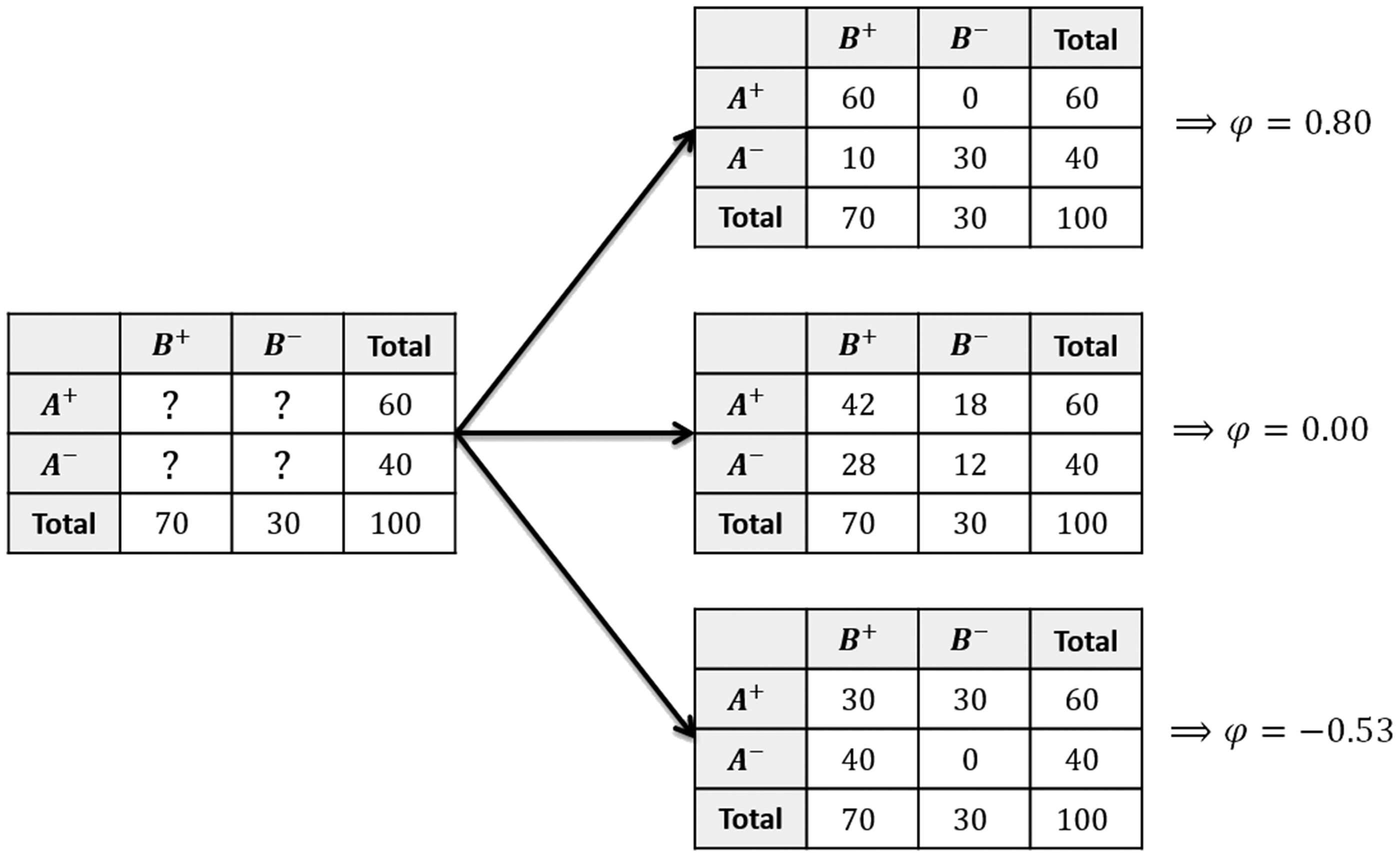

In order to use an informed account of the correlations while employing the correct likelihood of the data described in equation (6), we instead utilize external information for ϕ. In section 3.6, we discuss how to formulate prior distributions for this quantity based on external data or expert opinion. Given $p_{A}$ , $p_{B}$ and ϕ, we calculate $p_{1} = p_{A} p_{B} + ϕ \sqrt{p_{A} (1 - p_{A}) p_{B} (1 - p_{B})}$ , $p_{2} = p_{A} - p_{1}$ , $p_{3} = p_{B} - p_{1}$ and $p_{4} = 1 - p_{1} - p_{2} - p_{3}$ . This method allows for an informed reconstruction of the full contingency table. This is performed in a stochastic way: more plausible configurations (according to the prior) are given a higher probability. Note that given a set of values for $p_{A}$ and $p_{B}$ , ϕ is bounded between a minimum and a maximum value.^30,31 Thus, after drawing values for the model's parameters from the corresponding prior distributions, values the prior distribution for ϕ need to be appropriately truncated. Finally, note that when one (or more) of the margins is 0, then the contingency table can be reconstructed with certainty. For the reader's convenience, we provide the full likelihood of the model in the online Appendix, section 2.

An alternative method for reconstructing the 2 × 2 table uses the odds-ratios of the cross-classified information instead of ϕ. The advantage of this method is that it does not require any truncation. The disadvantage is that it is less easy to formulate clinically meaningful priors for the parameters. Details on this alternative approach are presented in section 3 of the online Appendix.

3.4 Mixed design

We now move on to the situation where a study includes a mixture of bilateral and unilateral interventions (mixed-design studies). For including this type of studies in the analysis, we will make one extra assumption. We will assume that in each such study, the probability of having an event when receiving a specific intervention is the same in patients receiving unilateral interventions (patients receiving only that intervention) and bilateral interventions (patients receiving both interventions): $p_{A}^{unil} = p^{bilat} (A^{+} | B^{+}) p^{bilat} (B^{+}) + p^{bilat} (A^{+} | B^{-}) p^{bilat} (B^{-}) \equiv p_{A}$ . This assumption might not hold if there is an interaction between the two interventions, for patients who received both. In such case, additional assumptions would be needed. Note that for the case of zero correlation, we would have $p^{bilat} (A^{+} | B^{+}) = p^{bilat} (A^{+} | B^{-})$ .

In what follows, we suppress the study index. Let us start by assuming that such a study provides all relative information, i.e. the number of patients who only received intervention A, the number of patients who only received B, as well as the number of patients who received both A and B; also, the number of events for each of these three patients groups, and the full cross-classifications for the bilateral interventions. We can estimate relative effects from such a study by employing the methods described in the previous sections, namely two independent binomial likelihoods for the unilateral interventions in A and B, and a multinomial likelihood as in equation (5) for the bilateral ones. If no information on the cross-classifications is available, likelihood (equation (6)) needs to be used instead, together with some external information on the correlation coefficient. According to our assumptions, these three groups inform only two probability parameters, $p_{A}$ and $p_{B}$ .

Let us now focus on an even more complicated scenario, which also corresponds to the seven mixed-design studies in the CTS example. More precisely, let us assume that such a study provides information on the events on each intervention ( $r_{A}, r_{B}$ ), the total number of patients receiving each intervention ( $N_{A}, N_{B})$ and the total number of patients in the study (N). The number of events and the number of patients with a unilateral intervention (A and B), and the number of events and patients with a bilateral intervention are not reported.

We first need to calculate the number of patients who received unilateral and bilateral interventions, using the reported data. Let us keep in mind that each patient can have a maximum of one event per intervention. Let us denote $N_{A}^{u}$ ( $N_{B}^{u}$ ) the number of patients who received only intervention A (B). Let $N^{b}$ denote the bilateral interventions, i.e. the number of patients who received both A and B. Obviously $N_{A}^{u} + N_{B}^{u} + N^{b} = N$ . It also holds that $N_{A}^{u} + N^{b} = N_{A}$ and $N_{B}^{u} + N^{b} = N_{B}$ . By solving this set of equations, we find the number of patients in each group, i.e. $N_{A}^{u} = N - N_{B}$ , $N_{B}^{u} = N - N_{A}$ and $N^{b} = N_{A} + N_{B} - N .$

We do not have information on how the $r_{A}$ events in intervention A are divided among the $N_{A}^{u}$ patients who received only A and the $N^{b}$ patients who received both A and B. Let us assume that x out of these $r_{A}$ events were in the $N_{A}^{u}$ patients; the rest $r_{A} - x$ were in the $N^{b}$ bilateral cases. Obviously, it should hold that $x < N_{A}^{u}$ . Also $r_{A} - x < N^{b},$ i.e. the number of events in the bilateral interventions group must be smaller than the total number of patients in that group. Of course $x \geq 0$ and also $x \leq r_{A}$ . All these constraints are summarized in the following double inequality: $max (0, r_{A} - N^{b}) \leq x \leq min (N_{A}^{u}, r_{A})$ . Likewise, if we denote by y the number of patients who only received intervention B and had an event, it holds that $max (0, r_{B} - N^{b}) \leq y \leq min (N_{B}^{u}, r_{B})$ .

We also do not know how the $r_{A} - x$ and $r_{B} - y$ events observed in patients who received bilateral interventions are cross-classified in a $2 \times 2$ contingency table, like the one in Table 1. In Figure 2, we give a graphical analysis of the possible ways that the observed events may be distributed in each category of patients.

Figure 2.

Graphical analysis of the different ways in which the observed events can be distributed among different categories of patients in a mixed-design study. x, y and n₁ are not reported.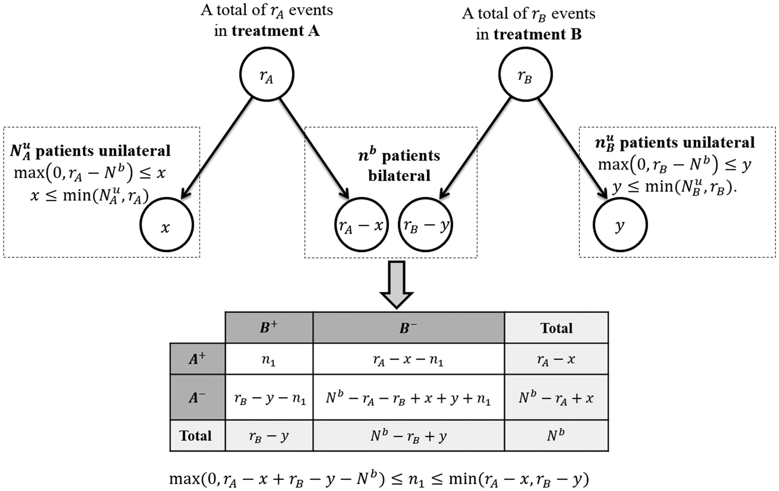

Quantities 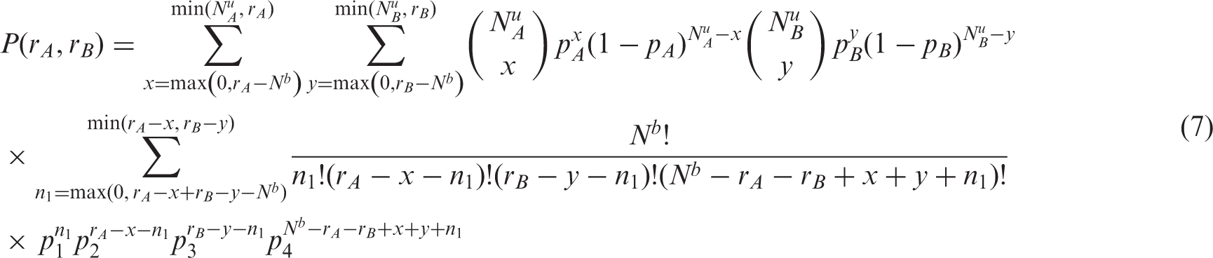$x, y$ and $n_{1}$ of Figure 2 are not reported. In order to write the exact likelihood of the reported data ( $r_{A}, r_{B}$ , $N_{A}, N_{B}$ and N), we will combine the likelihoods of all possible configurations that lead to these observations, as presented in Figure 2. Since x and y correspond to events in different groups of patients, they follow independent binomial distributions i.e. $x \sim Bin (p_{A}, N_{A}^{u})$ and $y \sim Bin (p_{B}, N_{B}^{u})$ . For the events in the group of patients with bilateral interventions, we follow the analysis of section 3.3 and we can write the likelihood after carefully adjusting equation (6). The full, exact likelihood of the observed data ( $r_{A}$ , $r_{B}$ ) can be written as

\begin{array}{l} P (r_{A}, r_{B}) = \sum_{x = \max (0, r_{A} - N^{b})}^{min (N_{A}^{u}, r_{A})} \sum_{y = \max (0, r_{B} - N^{b})}^{min (N_{B}^{u}, r_{B})} (\begin{matrix} N_{A}^{u} \\ x \end{matrix}) p_{A}^{x} {(1 - p_{A})}^{N_{A}^{u} - x} (\begin{matrix} N_{B}^{u} \\ y \end{matrix}) p_{B}^{y} {(1 - p_{B})}^{N_{B}^{u} - y} \\ \times \sum_{n_{1} = max (0, r_{A} - x + r_{B} - y - N^{b})}^{min (r_{A} - x, r_{B} - y)} \frac{N^{b}!}{n_{1}! (r_{A} - x - n_{1})! (r_{B} - y - n_{1})! (N^{b} - r_{A} - r_{B} + x + y + n_{1})!} \\ \times p_{1}^{n_{1}} p_{2}^{r_{A} - x - n_{1}} p_{3}^{r_{B} - y - n_{1}} p_{4}^{N^{b} - r_{A} - r_{B} + x + y + n_{1}} \end{array}

(7)

This likelihood is a generalization of the cases described in sections 3.1 (unilateral interventions only) and 3.3 (bilateral interventions only). It is easy to see that this likelihood decomposes into a simple product of two independent binomials if we set $N^{b} = 0$ (in which case $x = r_{A}, y = r_{B}$ and $n_{1} = 0$ ): this corresponds to the case where there are no bilateral interventions. It is also straightforward to see that if we set $N^{b} = N$ then $N_{A}^{u} = N_{B}^{u} = x = y = 0$ and the likelihood of equation (7) reduces to the one of equation (6), as expected. A more detailed description of this model can be found in section 4 of the online Appendix.

The joint posterior distribution for $p_{A}$ and $p_{B}$ includes their correlation. The extent of this correlation depends on (1) the number of patients who received bilateral interventions in the studies, where zero bilateral interventions will mean zero correlation and (2) the prior distribution used for ϕ.

3.5 Unknown design

A study of this type reports $r_{A}, r_{B}$ , $N_{A}$ and $N_{B}$ , but does not provide any information on the total number of patients. This implies that there is no (exact) information on how many of the included patients received unilateral and how many bilateral interventions; but meta-analysts might have reasons to suspect that at least some of the patients in these studies received both interventions.

The lack of more information from these studies means that researchers cannot use the methods described in the previous sections to take into account correlations in the estimation of relative intervention effects, unless some strong assumption is employed, i.e. on the percent of bilateral interventions in the study. The simplest approach for the analysis is to assume two independent binomials. As we discussed, this may lead to over- or under-precision in the estimated relative intervention effects if the correlation is non-zero.

The two extreme cases for such a study are (1) there are no bilateral interventions and (2) there are a maximum number of bilateral interventions ( $= max (N_{A}, N_{B}))$ . Given that information on this number is unavailable, when analysing such a study researchers may want to use the most conservative estimate. This means that if $p_{A}$ and $p_{B}$ are expected to be positively correlated in bilateral interventions, the analyst should analyse a study of unknown design as if all patients received only one intervention, i.e. as if the study was unilateral. If instead researchers are interested in obtaining the most liberal estimates, they should assume that a large number of interventions might be bilateral (maximum value is $max (N_{A}, N_{B})$ ). These considerations need to be reversed for the (perhaps less relevant) case of having a negative correlations. In any case, a sensitivity analysis is warranted to explore the effect of the (unknown) study design in the overall, pooled effect.

In section 5 of the online Appendix, we provide a summary table of how to choose the likelihood for each study, depending on its design and on the information it provides.

3.6 Formulating informative prior distributions

In what follows, we discuss how meta-analysts can augment the information included in the studies using external information in the form of informative prior distributions for the model parameters. We focus on one-step meta-analysis models. We discuss the following parameters: the heterogeneity variance, the mean and variance of the average risk and the correlation (ϕ coefficient).

3.6.1 Heterogeneity

In a recent meta-epidemiological study by Turner et al.,³² the authors re-analysed data from around 15,000 binary outcome meta-analyses from the Cochrane Database of Systematic Reviews. Results were used to create informative predictive distributions for $τ^{2}$ .³³ These prior distributions cover 80 different settings, categorized by the outcome being assessed, the types of interventions being compared, etc.

3.6.2 Average risk

The optimal source of information for this parameter would be to use eligible randomized controlled trials that were excluded from the original meta-analysis due e.g. to inadequate reporting of effect sizes. This would allow researchers to obtain a realistic estimate of the mean and variance of the (logit-transformed) average risk in order to formulate priors that can be included in the model. Alternatively, one could use observational studies (such as registries or large cohort studies). Note, however, that in order to formulate a prior distribution for the variance (parameter $σ_{u}$ in equation (2)), one would need to include multiple studies. If no external source of information is readily available, then a prior distribution can be elicited from the experts, following a method described in Efthimiou et al.²⁵ and Garthwaite et al.³⁴ In section 6 of the online Appendix, we discuss the details of this method, i.e. how researchers can elicit information and how they can synthesize information obtained from multiple experts (after possibly weighting each expert's opinion, e.g. for the years of experience on the field or the number of studies he/she has been involved in).

3.6.3 Correlation

If some of the studies report full, cross-classified information (as described in section 3.2), then the corresponding estimates of the correlation coefficients can be used to formulate an informative prior distribution for the analysis of the rest of the studies. Alternatively, one can formulate priors by eliciting information from expert clinicians. In a previous work, we describe how to elicit information on correlation indirectly, using a conditional probability.²⁵ Here, we propose a more straightforward method. As shown empirically by Clemen et al.,³⁵ directly asking for the correlations is a reasonable approach, often more accurate than indirect methods. More detail on how to synthesize information from multiple experts in order to construct a prior distribution for ϕ can be found in section 7 of the online Appendix. The method uses the Fisher transformation to synthesize information, $ζ = \frac{1}{2} log (\frac{ϕ + 1}{1 - ϕ})$ . If there is no usable external information for ϕ, researchers can use a minimally informative prior $ϕ \sim U (0, 1)$ if the correlation is generally expected to be positive (and conversely $ϕ \sim U (- 1, 0)$ if it is expected to be negative).

It is unclear whether the choice of the prior distribution for the different parameters of our model is equally important, and whether researchers should focus on obtaining informative priors for some of the parameters rather than others. It is also unclear what would be the impact of using misspecified prior distributions to our model estimates. Lambert et al.³⁶ showed that in general the choice of scale parameters (such as standard deviations) is more important than the choice of location parameters in Bayesian analyses with sparse data. As we will see in the next section, this agrees with the findings of our simulations. There we discuss that heterogeneity is the most influential parameter in our model. Using an informative prior for heterogeneity can greatly increase precision and enhance the power of the model. As we will also see, using minimally informative (or even misspecified) priors for the rest of the parameters may have a smaller impact on the model's performance.

4 Simulations

4.1 Data generation procedure and description of the scenarios

We performed a small-scale simulation study to assess the performance of the model we proposed in this paper. We limited the simulations to the case of studies with bilateral design where only the marginal numbers of events are reported, and among which there is variability (heterogeneity). We explored a range of different scenarios. For each scenario, we simulated 100 datasets, with each dataset corresponding to an independent meta-analysis.

Scenarios 1–20 aimed to compare our model with the bivariate beta-binomial model. This model has been previously recommended for meta-analysing rare events.⁸ For these scenarios, we simulated 20 studies for each meta-analysis. Two additional scenarios (21 and 22) aimed to explore the importance of specifying informative priors for the parameters of our bivariate binomial model. For these scenarios, we simulated 10 studies for each meta-analysis, aiming to increase the impact of the prior distributions.

To generate data, for each scenario, we first defined the true relative treatment effect on the log-OR scale (μ), the log-odds of the average risk of event and its standard deviation $(μ_{u}, σ_{u})$ and also the correlation between the events (ϕ). For each independent meta-analysis, we sampled the variance of random effects from a log-normal distribution: $τ^{2} \sim LN (- 2, 1.5)$ .³³ Suppressing the study index for clarity, for each study, we sampled the study-specific treatment effects, $θ \sim N (μ, τ^{2})$ and the log-odds of the average risk, $u \sim N (μ_{u}, σ_{u}^{2})$ . We simulated the number of patients (N) in each study by drawing from a uniform distribution, $U (50, 100)$ .

Using $θ, u$ and ϕ, we calculated the probabilities $p_{1}$ , $p_{2}$ , $p_{3}$ and $p_{4}$ (corresponding to $n_{1}$ , $n_{2}$ , $n_{3}$ and $n_{4}$ of Table 2). Using these four probabilities and the number of patients per study, we generated the number of events of the 2 × 2 cross-classified table by drawing from a multinomial distribution. We then calculated $r_{A}, r_{B}$ ; together with $N,$ these are the only data that were supposed to be available from the study.

We explored scenarios using the following values for the simulation parameters:

$μ = 0, 0.5$ .

$ϕ = 0.30 (ζ = 0.31$ , low correlation) and $ϕ = 0.60 (ζ = 0.69$ , high correlation).

$μ_{u} = - 1.5$ , $σ_{u} = 0.5$ : in these scenarios, there were almost no single- and double-zero studies (<1%). $μ_{u} = - 3.0, - 3.5$ and $σ_{u} = 1.0$ : these scenarios have some single- and double-zero studies (0 – 30% in total). $μ_{u} = - 4.0$ , $σ_{u} = 1.0$ and $μ_{u} = - 3.0$ , $σ_{u} = 3.0$ : these scenarios have many single- and double-zero studies (more than 30% in total).

We generated all data in R,³⁷ code is provided in the online Appendix, section 8.

4.2 Analyses of the simulated datasets

The simulated datasets were analysed using the bivariate binomial model discussed in section 3.2. The model is also presented in more detail in section 2 of the online Appendix. We performed our analyses in OpenBUGS,^38,39 the code is available in section 9 of the online Appendix. For each analysis, we simulated a single chain of 20,000 samples, and we discarded the first 5,000 samples. This was deemed to be sufficient based on some initial runs and also after visually inspecting the posterior distributions.⁴⁰

For the analysis of scenarios 1–20, we chose between using weakly informative prior distributions centred near the true value of the parameters, vague priors and misspecified priors for the correlation. These choices are described in detail in Table 4 of the online Appendix (section 10.1). In addition, these scenarios were analysed using the bivariate (Sarmanov) beta-binomial model, which accounts for correlations in the 2 × 2 tables.²¹ For this, we used a routine in R³⁷ provided by Chen et al.²¹ We also checked results by comparing with results obtained from the mmeta package in R, which also implements the beta-binomial model.⁴¹ We compared our model with beta-binomial in terms of (a) mean bias; (b) mean squared error (MSE) (the mean of the squared bias); (c) empirical coverage (the percent of meta-analyses that included the true effect in their 95% credible interval (CrI)); (d) empirical power (percent of meta-analyses that rejected the null hypothesis of no treatment effect, when the true treatment effect was non-zero); and (e) the gain in precision (bivariate binomial model over beta-binomial model). This was calculated as the percentage reduction of the mean width of the 95% CrI obtained from our model as compared to the 95% confidence interval from the beta-binomial model. The datasets generated under scenarios 21 and 22 were analysed multiple times, using only the model presented in this paper. Each dataset was analysed using first vague priors for all parameters, and then using vague priors for all model parameters except for one at a time. Details can be found in Table 5, section 10.2 of the online Appendix.

Table 4.

Results from analysing scenarios 21 and 22, for different choices of priors for the model parameters.^a

No.	Scenario	Informative priors used for	Mean bias	MSE	Coverage	Power	Increase in precision compared to non-informative priors
21	μ = 0.5, φ = 0.3 Many SZ/DZ	–	0.067	0.250	94%	25%	(reference)
		τ ²	0.016	0.210	90%	41%	30%
		φ	0.055	0.227	97%	21%	0%
		μ_u and σ_u	0.056	0.227	95%	27%	5%
22	μ = 0.5, φ = 0.6 Many SZ/DZ	–	0.094	0.146	96%	25%	(reference)
		τ ²	0.046	0.114	90%	55%	29%
		φ	0.078	0.132	98%	21%	0%
		μ_u and σ_u	0.068	0.124	96%	26%	5%

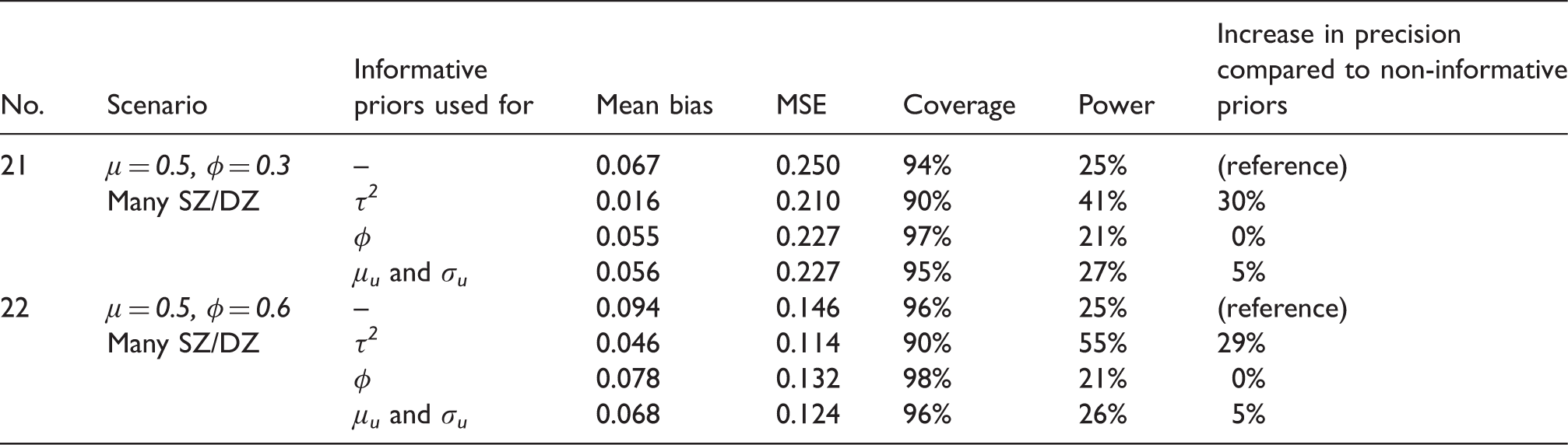
MSE: mean squared error.

μ denotes the log-odds ratio and φ the correlation. μ_u and σ_u denote the mean and standard deviation of the average risk.

4.3 Results from the simulations

The results from the analyses of scenarios 1–20 are presented in Table 3. Regarding the interpretation of results, and taking scenario 1 as an example, we can see that our model had a slightly larger mean bias for the logOR than the bivariate beta-binomial (0.012 vs. 0.001), and also a slightly larger MSE (0.024 vs. 0.018). However, the CrIs obtained from our model were narrower than the confidence intervals obtained from the bivariate beta-binomial model. Thus, coverage for the former model was 95% while for the latter it was 99%. By comparing the precision of the two models (quantified by the width of the corresponding credible/confidence intervals), we calculated a 29% increased precision of our model as compared to the bivariate-binomial.

Table 3.

Results from 20 scenarios, comparing the proposed bivariate binomial model to the bivariate beta-binomial model.^a

			Bivariate binomial				bivariate beta-binomial
#	Scenario description		Mean bias	MSE	Coverage	Power	Mean bias	MSE	Coverage	Power	Precision gained
μ = 0
1	φ = 0.3	No SZ/DZ	0.012	0.024	95%	-	0.002	0.018	99%	-	29%
2		Some SZ/DZ	0.006	0.044	96%	-	0.000	0.030	100%	-	30%
3		Many SZ/DZ	0.031	0.059	96%	-	0.017	0.055	98%	-	29%
4	φ = 0.6	No SZ/DZ	0.000	0.022	98%	-	0.007	0.010	100%	-	27%
5		Some SZ/DZ	0.006	0.032	95%	-	0.008	0.029	99%	-	41%
6		Many SZ/DZ	0.002	0.031	95%	-	0.004	0.024	99%	-	38%
μ = 0.5
7	φ = 0.3	No SZ/DZ	0.017	0.024	96%	90%	0.043	0.013	98%	53%	31%
		Some SZ/DZ and:					0.042	0.056	100%	16%
8		Informative priors	0.022	0.054	95%	69%					39%
9		Vague priors	0.037	0.069	97%	56%					22%
10		Misspecified priors	0.014	0.050	97%	59%					36%
11		Many SZ/DZ	0.026	0.079	91%	59%	0.005	0.077	97%	13%	34%
12	φ = 0.6	No SZ/DZ	0.006	0.016	98%	90%	0.052	0.015	100%	49%	43%
		Some SZ/DZ and:					0.040	0.047	98%	12%	44%
13		Informative priors	0.008	0.054	95%	82%
14		Vague priors	0.035	0.062	97%	75%					32%
15		Misspecified priors	0.017	0.048	98%	67%					33%
16		Many SZ/DZ	0.076	0.066	91%	71%	0.033	0.064	99%	17%	43%
μ = 0.5. Assumed large σ_u (variability in the average risk)
17	φ = 0.3	Many SZ/DZ	0.000	0.063	97%	44%	0.258	0.103	81%	1%	18%
18	φ = 0.3	Some SZ/DZ	0.024	0.028	98%	77%	0.221	0.071	95%	1%	39%
19	φ = 0.6	Many SZ/DZ	0.040	0.071	96%	60%	0.242	0.112	86%	2%	29%
20	φ = 0.0	Many SZ/DZ	0.011	0.046	100%	45%	0.260	0.101	87%	0%	25%

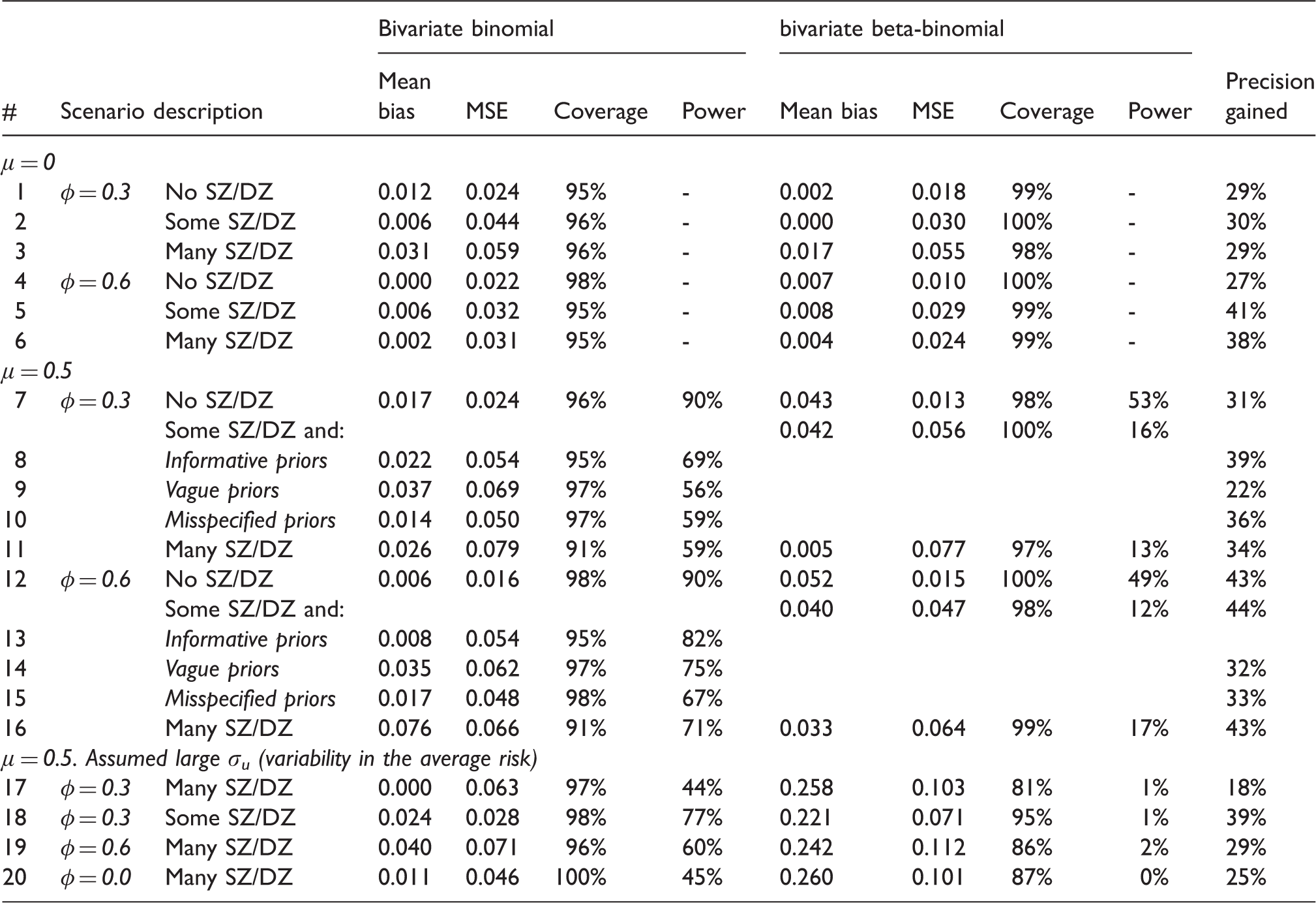
CrI: credible interval; MSE: mean squared error.

All scenarios are analysed using informative priors on φ for the bivariate binomial model, except otherwise noted. SZ (DZ): single (double)-zero studies. ‘Some SZ/DZ’ denotes scenarios with 0–30% SZ/DZ studies. ‘Many SZ/DZ’ denotes scenarios with >30%. μ denotes the true log-odds ratio, φ the true correlation in each scenario and σ_u the standard deviation of the log-odds of the average risk. Large heterogeneity in average risk corresponds to σ_u > 2. Gain in precision corresponds to the percentage reduction in the width of the 95% CrI of our model vs. the beta-binomial.

Simulations showed that our model performs markedly better than the beta-binomial model in most scenarios we explored. In almost all cases, our approach led to smaller mean bias and similar MSE. Coverage probability was closer to the nominal 95% in our approach for most scenarios. Our model led to an increased precision of the estimates. This increase in precision, quantified as the percentage reduction of the width of the 95% CrI, ranged from 29 to 44% in all scenarios. Our approach performed much better in scenarios with many single- and double-zero studies, when we assumed non-zero log-ORs. In these settings, the beta-binomial model had very low power to detect a relative treatment effect. Our simulations showed that in the presence of bilateral interventions, even when the prior distributions are only mildly informative or misspecified, the bivariate binomial model performs better than the bivariate beta-binomial (Scenarios 13–16).

Another interesting finding in our simulations was that for the case of non-zero relative treatment effects and large heterogeneity in the average risk (Scenarios 17–20), the beta-binomial model was very inefficient. In these scenarios, this model showed excessive bias, and in all cases, the bias was towards zero treatment effects. Moreover, there was large MSE, insufficient coverage and minimal power. This was the case even under zero correlation scenario, i.e. for the usual unilateral design (Scenario 20). This finding comes in contrast with the recommendations by Kuss,⁸ i.e. to use the beta-binomial model for all meta-analyses of rare events. But, in his simulations,⁸ Kuss did not explore the scenario of large heterogeneity in the average risk of an event. In a somewhat different context (meta-analysis of proportions, not relative effects), Ma et al. showed that the beta-binomial model performs worse when the event rates are relatively large (e.g. >5%).⁴²

In Table 4, we present the results from the analysis of data simulated under scenarios 21 and 22, using different priors for the model's parameters. Results suggested that the most influential prior is the one for heterogeneity. Using an informative prior distribution for $τ^{2}$ instead of a vague one greatly enhanced the performance of the model in terms of bias, precision, coverage and power. Using informative priors for the other model, parameters had a smaller impact in all scenarios explored.

5 Applications

In this section, we show results from applying our methods to the two examples presented in section 2. We used the following models for the analysis:

Univariate fixed-effects meta-analysis, i.e. we used model in equation (2), but omitting the random effects distribution. This analysis ignores the correlations due to bilateral interventions. We fitted this model in a Bayesian as well as a frequentist setting, using maximum likelihood estimation (MLE).

Univariate random effects meta-analysis (UNI-RE), using the model in equation (2). This analysis ignores the correlations due to bilateral interventions. We fitted this model in a Bayesian as well as a frequentist setting, using MLE.

Bivariate binomial, fixed-effects meta-analysis: we used the model described in this paper accounting for the correlations due to bilateral interventions, as discussed in sections 3.3 and 3.4. We omitted random effects.

Bivariate binomial, random effects meta-analysis (BB-RE): the same as in model 3, but also including random effects

The bivariate beta-binomial model. Note that this is by definition a random effects model.

We provide the OpenBUGS code in section 11 of the online Appendix. In section 12 of the online Appendix, we provide codes for fitting the model in R using the R2WinBUGS package,⁴³ and for fitting the model of equation (2) in a frequentist setting. We performed 20,000 iterations, and we discarded the first 5000 samples. We fitted the bivariate beta-binomial model in R.²¹ We fitted all models using a conventional laptop computer. The run-time required for fitting our bivariate binomial model was around 23 min for the CTS example and less than a minute for the myopia example.

5.1 Surgical operations for CTS

Two studies in this dataset had unclear design. We analysed these studies as if they were of unilateral design following the arguments presented in section 3.5 as we expect a positive correlation between complications in two arms of the same patient.

For models 1 to 4, we assume a vague prior $μ_{u} \sim U (- 6, 0)$ for the log-odds of the mean event rate, $σ_{u} \sim U (0, 3)$ for the corresponding variance and $μ \sim U (- 2, 2)$ for the log-OR. For the random effects models (models 2 and 4), we use informative priors from the empirical distributions for a safety outcome for non-pharmacological interventions $log (τ^{2}) \sim N (- 1.43, 1 . 45^{2})$ provided in Turner et al.³³ For the bivariate models (3 and 4), we perform two analyses: one assuming a low correlation between the outcomes, $ζ \sim N (0.2, 0 . 1^{2})$ , and one assuming a moderate-high correlation, $ζ \sim N (0.5, 0 . 1^{2})$ . Results are in Figure 3. The BB-RE model with moderate-high correlation was assumed to be our primary model, the rest of the models can be seen as sensitivity analyses. For the primary model, the posterior median estimate for $μ_{u}$ was –3.41 (–4.35, 2.56) and for $σ_{u}$ was 1.93 (1.33, 2.80).

Figure 3.

Meta-analysis for minor events, endoscopic vs. open surgical operation for CTS, using a range of alternative models: UNI-FE (B/F): univariate fixed-effect (Bayesian/Frequentist), UNI-RE (B/F): univariate random effects (Bayesian/Frequentist), BB-FE: bivariate binomial fixed-effect (Bayesian), BB-RE: bivariate binomial random effects (Bayesian). For all Bayesian models, we present the median of the posterior distribution.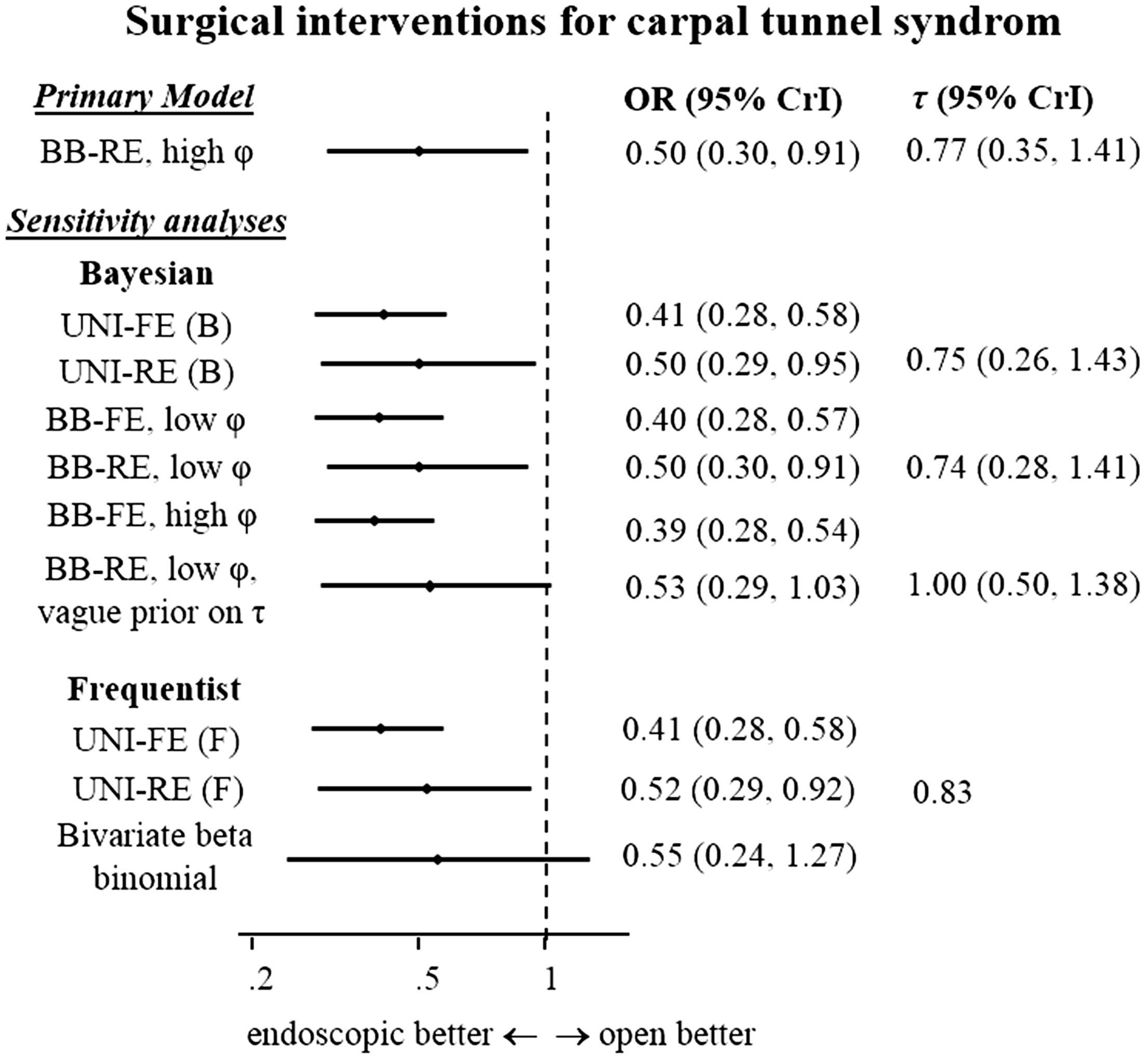

The endoscopic surgical operation was found to be more safe than the open in all analyses. When switching from the univariate to the bivariate model, the increase in precision was rather small, especially when a low correlation was assumed. This should come as no surprise, as only 13% of the patients in this meta-analysis received bilateral interventions. One interesting observation was that when we increase the assumed correlation in the BB-RE scenario, the estimate and CrI for the OR remained unchanged. This is because the increased precision in study-estimates is accompanied by an increase in the estimated heterogeneity. All implementations of the bivariate binomial model were more precise than the beta-binomial model. Comparing the Bayesian and frequentist implementations of the UNI-RE model, we see some differences, which reflect the impact of the prior distributions. E.g. the MLE estimate for τ in the UNI-RE (F) model was 0.83, while for UNI-RE (B), the median of the posterior median for τ was 0.75. This difference was due to the impact of the informative prior distribution, which has median 0.48, thus pulling the MLE estimate towards lower values. The estimate for the ORs was also slightly different (0.50 for the Bayesian implementation vs. 0.52 for the frequentist). This difference can be attributed to the prior used for logOR, which was centred at 0, thus pulling the MLE estimate to lower values.

In order to assess the impact of the prior distributions in our results, we did a sensitivity analysis for model 4 (BB-RE) with low correlation. Assuming vague priors for μ, $μ_{u}$ and $σ_{u}$ had an immaterial impact on the results. However, a less informative prior for the heterogeneity ( $τ^{2} \sim U (0, 2)$ ) considerably increased imprecision in the treatment effects. This highlights once more the importance of using informative prior distributions specifically for the random effects variance parameter.

Finally, as we argued in section 3.3, the only information the data carries for the correlation coefficient ζ is the range of the allowed values within each study determined by the marginal total counts (as also depicted in Figure 1). As a result, the posterior estimates for ζ are entirely determined by their prior distributions.

5.2 Surgical techniques for correcting myopia

Two studies in this dataset had unclear design. We analysed these studies as if they were of unilateral design. We used the following prior distributions for the model parameters: $μ_{u} \sim U (- 5, 5)$ ; $σ_{u} \sim U (0, 5)$ and $μ \sim U (- 2, 2)$ . For heterogeneity, we use an informative prior distribution $log (τ^{2}) \sim N (- 1.69, 1 . 68^{2})$ based on the empirical evidence.³³ We explore two options for correlation, $ζ \sim N (0.2, 0 . 1^{2})$ (low correlation), and $ζ \sim N (0.5, 0 . 1^{2})$ (moderate-high correlation). Results are presented in Figure 4. For our primary model, the posterior median estimate for $μ_{u}$ was 1.35 (–0.16, 2.99) and for $σ_{u}$ was 2.20 (1.34, 3.90).

Figure 4.

Meta-analysis for uncorrected visual acuity (UCVA) of 20/20 or better, at six months after treatment, LASIK vs. PRK for myopia. Model abbreviations as per Figure 3.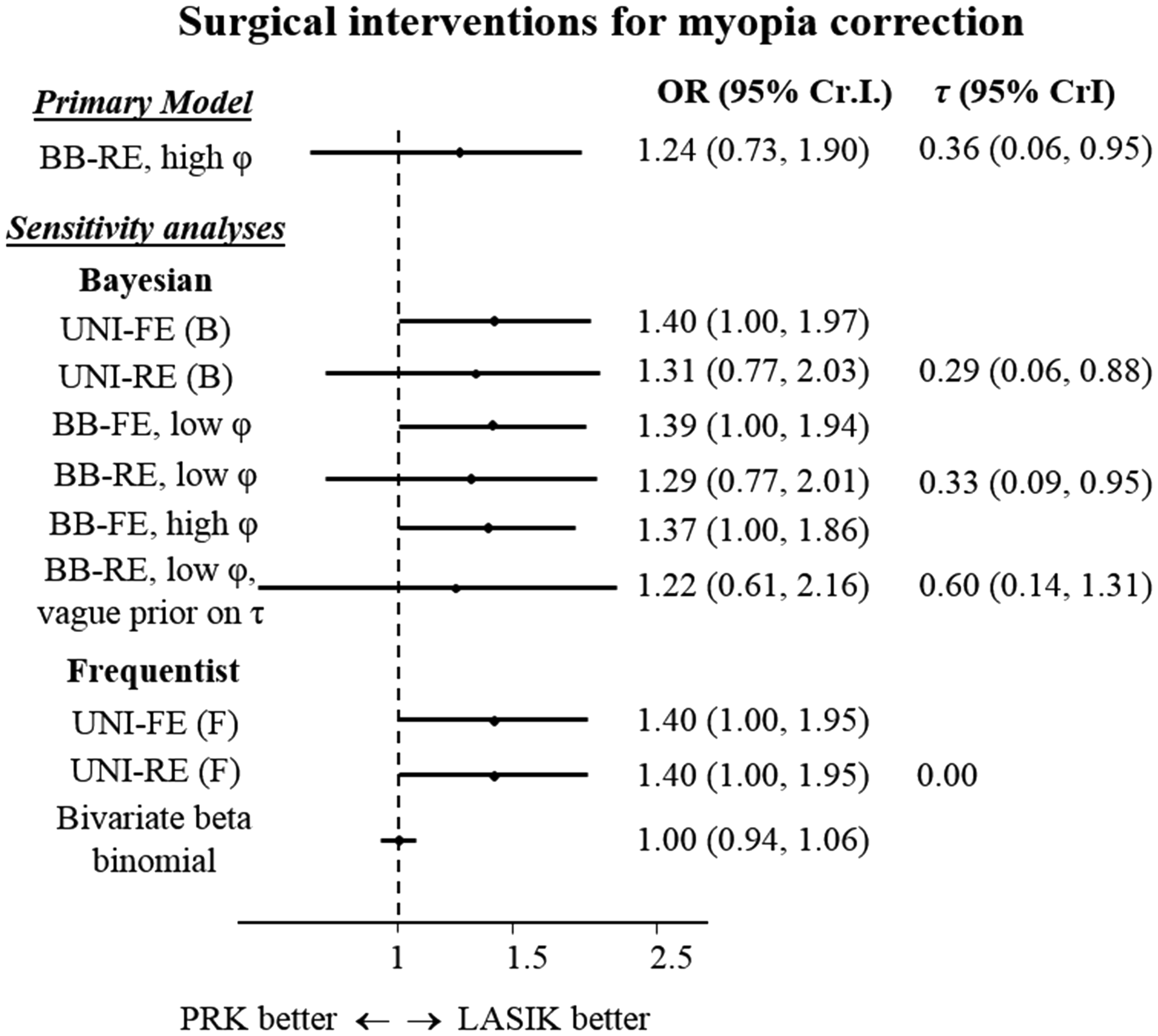

Accounting for correlations using our approach led to an increase in precision of the pooled estimates. For the case of random effects model, some of the increase in precision was again counterbalanced by an increase in the estimates for $τ^{2}$ , as in the CTS example. There are some differences between Bayesian and frequentist implementations of the UNI-RE model, particularly for τ. Heterogeneity was estimated to be 0 in the frequentist implementation, while in the Bayesian approach, the median posterior τ was 0.29. This difference is again due to the effect of the informative prior distribution (which had a median of 0.43).

The OR estimated from the beta-binomial model was 1.00 (0.94, 1.06). This finding was markedly different to the results from all bivariate binomial models. It was also in disagreement with the frequentist analysis performed in the original publication; the authors performed a Mantel-Hanszel fixed-effects meta-analysis resulting into OR = 1.40 (1.00, 2.00), which is in broad agreement with bivariate binomial models.

One explanation for this important discrepancy between beta-binomial and the other approaches lies in the distribution of the average risk in the included studies. The average event risk ranged from 8 to 97% in the included studies, despite the fact that the relative treatment effect was not very heterogeneous (see online Appendix, section 1.2). In such situations, the bivariate beta-binomial model may be heavily biased towards zero, as shown in the simulations (section 4, scenarios 17–20). Additionally, the bivariate beta-binomial model was shown to perform well when the event rate is small; here it is on average 70%.⁴²

6 Discussion

In this paper, we have presented a Bayesian meta-analysis model for synthesizing binary data obtained from collection studies of different designs: studies of the usual parallel design, studies of a bilateral (split-body) design and studies including a mixture of unilateral and bilateral interventions. Our model uses a bivariate binomial distribution that accounts for the correlations induced due to bilateral operations and has several distinct advantages. It uses the exact likelihood of the data; it does not employ the normal approximation; it respects the randomization of the studies; it includes in the analysis data coming from studies with zero events in one or even both interventions, without a need for imputation. Our model has similarities with the bivariate beta-binomial (Sarmanov) model for meta-analysis (e.g. as described by Chen et al.²¹). The two models differ, however, in the model parametrisation and the assumption of random effects. The bivariate beta-binomial model assumes random effects for the arm-specific event probabilities while the mean log-OR is not a parameter of the model. In our approach, random effects are assumed for study-specific log-ORs, and the mean log-OR is a parameter directly estimated in the model. This feature allows us to assume an informative prior distribution for the log-OR, based on available empirical distributions.

The bivariate beta-binomial model has been previously suggested as the optimal approach for meta-analysing rare events.⁸ Our simulations showed that our model may lead to significant increase in precision, coverage and power, and a decrease in bias, as compared to the bivariate beta-binomial model. Moreover, according to our simulations, the bivariate beta-binomial model was found to perform very badly when the baseline risk was very variable in the included studies, even when no correlation was assumed. This was also demonstrated in one of the two real data-sets we used to illustrate our methods. The increase of precision in our model is more pronounced in fixed-effects meta-analyses. In the random effects regime, increasing the precision of the study estimates by accounting for correlations can be partly counterbalanced by an increase in the estimate for heterogeneity.

We set our model in a Bayesian framework. This allows the inclusion of external information for the model parameters. However, for the case of rare events, inferences from Bayesian meta-analyses may heavily depend on the choice of prior distribution for the parameters – even when these are thought to be uninformative.³⁶ Due to this fact, the use of frequentist approaches instead of Bayesian approaches is sometimes advocated. We understand the reasoning behind this view; in this paper, however, we argue in favour of a Bayesian approach. We think that the scarcity of information due to the rarity of events should not be seen as an argument against the use of Bayesian methods. On the contrary, we think that meta-analysts should opt for using Bayesian methods when they have the opportunity to include high quality, trustworthy external evidence in the analysis.

The major limitation of our model lies on its complexity. The software code we provide might be computationally heavy when studies have very large sample sizes. This may be especially true if there are large, mixed-design studies in the dataset. Moreover, embarking into this complicated modelling will only make a difference in the estimates if the corresponding correlation is large. If the correlation is expected to be small (e.g. $ϕ < 0.2$ ), then researchers can safely treat observations from patients that received both interventions as if they corresponded to different patients.

In our model, we assumed exchangeability on the average risk. This might be a very strong assumption to make, e.g. if there are large differences in the randomization ratio across studies. Alternatively, researchers can assume exchangeability in the probability of having an event in one of the interventions, $p_{i, A}$ or $p_{i, B}$ in equation (2). Choosing between the two, however, might be important when the data are sparse. Thus, the choice should be ideally guided by the availability of trustworthy external information that can be used to formulate informative priors. Another limitation of our model is that it does not account for the ordering and timing of the treatments. E.g. there might be studies where the treatments were administered simultaneously and there might be studies where treatment A is given first and treatment B later, or vice versa, first B then A.

One additional limitation of our model is that it cannot correctly account for correlations induced by patients that received the same intervention in multiple sites of their bodies i.e. a classical cluster design (e.g. the same intervention in both hands, both eyes, multiple teeth, multiple people in a household, etc.). This situation requires an extension of the approach described in this paper. Other possible extensions of our bivariate binomial meta-analysis model relate to the case of two correlated outcomes (for studies of the usual, parallel design) and for the meta-analysis of twin studies. Also, our model can be extended for the meta-analysis of the accuracy of multiple diagnostic tests. Finally, it would be interesting to explore the use of the non-central hypergeometric distribution^15,44 for bilateral interventions, and compare it with the bivariate binomial approach described in this paper.

Dimou et al.⁴⁵ discuss an alternative method that can be used to fill the (unknown) cross-classified information in the contingency tables of studies that do not report it. Their method uses information from studies that report the full tables. When no studies report the full tables, the authors suggest the use of the iterative proportional fitting algorithm,⁴⁶ which is, however, based on strong assumptions. Both these methods do not account for uncertainty in the (unobserved) missing values of the contingency tables. Moreover, the methods described in that paper are not suitable to use in the case of rare events.

A different approach to synthesizing data from studies with bilateral design is to only use information on the number of discordant pairs,² i.e. the number of patients with an event in A but not in B, and the number of patients with an event in B but not in A. This approach, however, could not be used for the case where some studies in the meta-analysis are of a unilateral design, and/or some studies are of a mixed design. E.g. this approach could not have been used in the examples presented in this paper.

To summarize, we think that the model we presented constitutes the best available method for meta-analysing binary outcomes in the presence of bilateral (split-body) interventions, and that its implementation is in practice straightforward.

Footnotes

Acknowledgements

We would like to thank Nikolaos Pandis and Haris Vasileiadis for their help in choosing and interpreting the clinical examples we used.

Declaration of conflicting interests

The author(s) declared no potential conflicts of interest with respect to the research, authorship and/or publication of this article.

Funding

The author(s) disclosed receipt of the following financial support for the research, authorship, and/or publication of this article: OE was supported by the Swiss National Science Foundation (grant title: ‘Enhancing methods for evaluating the comparative safety of medical interventions’). GR was funded by the German Research Foundation (DFG) (grant RU 1747/1-2). GS is a Marie Skłodowska-Curie Fellow (MSCA-IF-703254).

Supplemental material

Supplemental material for this article is available online.

References

Pandis

Chung

Scherer

et al.

CONSORT 2010 statement: extension checklist for reporting within person randomised trials. BMJ 2017; 357: j2835.

Elbourne

et al.

Meta-analyses involving cross-over trials: methodological issues. Int J Epidemiol 2002; 31: 140–149.

Curtin

Elbourne

Altman

. Meta-analysis combining parallel and cross-over clinical trials II: binary outcomes. Stat Med 2002; 21: 2145–2159.

Jackson

Riley

White

. Multivariate meta-analysis: potential and promise. Stat Med 2011; 30: 2481–2498.

Riley

. Multivariate meta-analysis: the effect of ignoring within-study correlation. J R Stat Soc Ser A Stat Soc 2009; 172: 789–811.

Mavridis

Salanti

. A practical introduction to multivariate meta-analysis. Stat Method Med Res 2013; 22: 133–158.

Bhaumik

et al.

Meta-analysis of rare binary adverse event data. J Am Stat Assoc 2012; 107: 555–567.

Kuss

. Statistical methods for meta-analyses including information from studies without any events – add nothing to nothing and succeed nevertheless. Stat Med 2015; 34: 1097–1116.

Vandermeer

et al.

Meta-analyses of safety data: a comparison of exact versus asymptotic methods. Stat Method Med Res 2009; 18: 421–432.

10.

Sweeting

Sutton

Lambert

. What to add to nothing? Use and avoidance of continuity corrections in meta-analysis of sparse data. Stat Med 2004; 23: 1351–1375.

11.

Bradburn

Deeks

Berlin

et al.

Much ado about nothing: a comparison of the performance of meta-analytical methods with rare events. Stat Med 2007; 26: 53–77.

12.

Greenland

. Simpson's paradox from adding constants in contingency tables as an example of Bayesian noncollapsibility. Am Stat 2010; 64: 340–344.

13.

Simmonds MC and Higgins JP. A general framework for the use of logistic regression models in meta-analysis. Stat Method Med Res 2016; 25: 2858–2877.

14.

Rücker

Schwarzer

Carpenter

et al.

Why add anything to nothing? The arcsine difference as a measure of treatment effect in meta-analysis with zero cells. Stat Med 2009; 28: 721–738.

15.

Stijnen

Hamza

Ozdemir

. Random effects meta-analysis of event outcome in the framework of the generalized linear mixed model with applications in sparse data. Stat Med 2010; 29: 3046–3067.

16.

Böhning

Mylona

Kimber

. Meta-analysis of clinical trials with rare events. Biom J 2015; 57: 633–648.

17.

Cai

Parast

Ryan

. Meta-analysis for rare events. Stat Med 2010; 29: 2078–2089.

18.

Firth

. Bias reduction of maximum likelihood estimates. Biometrika 1993; 80: 27–38.

19.

Sarmanov

. Generalized normal correlation and two-dimensional Fréchet classes. Dokl Akad Nauk SSSR 1966; 168: 32–35.

20.

Molenberghs

Verbeke

. Models for discrete longitudinal data, New York: Springer, 2005. .

21.

Chen

Chu

Luo

et al.

Bayesian analysis on meta-analysis of case-control studies accounting for within-study correlation. Stat Method Med Res 2015; 24: 836–855.

22.

Vasiliadis

Georgoulas

Shrier

et al.

Endoscopic release for carpal tunnel syndrome. Cochrane Database Syst Rev 2014; 1: CD008265.

23.

Shortt

Allan

BDS

Evans

. Laser-assisted in-situ keratomileusis (LASIK) versus photorefractive keratectomy (PRK) for myopia. Cochrane Database Syst Rev 2013; 1: CD005135.

24.

Lunn

Barrett

Sweeting

et al.

Fully Bayesian hierarchical modelling in two stages, with application to meta-analysis. J R Stat Soc Ser C Appl Stat 2013; 62: 551–572.

25.

Efthimiou

et al.

An approach for modelling multiple correlated outcomes in a network of interventions using odds ratios. Stat Med 2014; 33: 2275–2287.

26.

Cramer

. Mathematical methods of statistics, Princeton: Princeton University Press, 1946.

27.

Aitken

Gonin

. XI. – on fourfold sampling with and without replacement. Proc R Soc Edinb 1936; 55: 114–125.

28.

Hamdan

. Canonical expansion of the bivariate binomial distribution with unequal marginal indices. Int Stat Rev Rev Int Stat 1972; 40: 277.

29.

Bayramoglu (Bairamov)

Kemalbay

. Some novel discrete distributions under fourfold sampling schemes and conditional bivariate order statistics. J Comput Appl Math 2013; 248: 1–14.

30.

Guilford

. The minimal phi coefficient and the maximal phi. Educ Psychol Meas 1965; 25: 3–8.

31.

Davenport

El-Sanhurry

. Phi/phimax: review and synthesis. Educ Psychol Meas 1991; 51: 821–828.

32.

Turner

Davey

Clarke

et al.

Predicting the extent of heterogeneity in meta-analysis, using empirical data from the Cochrane Database of Systematic Reviews. Int J Epidemiol 2012; 41: 818–827.

33.

Turner

Jackson

Wei

et al.

Predictive distributions for between-study heterogeneity and simple methods for their application in Bayesian meta-analysis. Stat Med 2015; 34: 984–998.

34.

Garthwaite

Kadane

O'Hagan

. Statistical methods for eliciting probability distributions. J Am Stat Assoc 2005; 100: 680–701.

35.

Clemen

Fischer

Winkler

. Assessing dependence: some experimental results. Manag Sci 2000; 46: 1100–1115.

36.

Lambert

Sutton

Burton

et al.

How vague is vague? A simulation study of the impact of the use of vague prior distributions in MCMC using WinBUGS. Stat Med 2005; 24: 2401–2428.

37.

R Core Team. R: a language and environment for statistical computing. R Foundation for Statistical Computing, Vienna, Austria, http://R-project.org (accessed 21 March 2017).

38.

Lunn

Thomas

Best

et al.

WinBUGS – A Bayesian modelling framework: concepts, structure, and extensibility. Stat Comput 2000; 10: 325–337.

39.

Lunn

Spiegelhalter

Thomas

et al.

The BUGS project: evolution, critique and future directions. Stat Med 2009; 28: 3049–3067.

40.

Raftery

Lewis

. How many iterations in the Gibbs sampler? In Bayesian Statistics 4, Oxford: Oxford University Press, 1992, pp. 763–773.

41.

Luo

Chen

et al.

mmeta: an R package for multivariate meta-analysis. J Stat Softw 2014; 56: 11.

42.

Chu

Mazumdar

. Meta-analysis of proportions of rare events–a comparison of exact likelihood methods with robust variance estimation. Commun Stat Simul Comput 2016; 45: 3036–3052.

43.

R2WinBUGS: A package for running WinBUGS from R | Sturtz | Journal of Statistical Software, https://jstatsoft.org/article/view/v012i03 (accessed 21 March 2017).

44.

Houwelingen

VCH

Zwinderman

Stijnen

. A bivariate approach to meta-analysis. Stat Med 1993; 12: 2273–2284.

45.

Dimou

Adam

Bagos

. A multivariate method for meta-analysis and comparison of diagnostic tests. Stat Med 2016; 35: 3509–3523.

46.

Deming

Stephan

. On a least squares adjustment of a sampled frequency table when the expected marginal totals are known. Ann Math Stat 1940; 11: 427–444.

Supplementary Material

Please find the following supplemental material available below.

For Open Access articles published under a Creative Commons License, all supplemental material carries the same license as the article it is associated with.

For non-Open Access articles published, all supplemental material carries a non-exclusive license, and permission requests for re-use of supplemental material or any part of supplemental material shall be sent directly to the copyright owner as specified in the copyright notice associated with the article.

0.00 MB

0.82 MB

A model for meta-analysis of correlated binary outcomes: The case of split-body interventions

Abstract

Keywords

1 Introduction

2 Example datasets

2.1 Two surgical treatments for carpal tunnel syndrome

2.2 Two surgical techniques for correcting myopia

3 Methods

3.1 Unilateral design

3.2 Bilateral design: studies providing cross-classified information

3.3 Bilateral design: studies that do not provide cross-classified information

3.4 Mixed design

3.5 Unknown design

3.6 Formulating informative prior distributions

3.6.1 Heterogeneity

3.6.2 Average risk

3.6.3 Correlation

4 Simulations

4.1 Data generation procedure and description of the scenarios

4.2 Analyses of the simulated datasets

4.3 Results from the simulations

5 Applications

5.1 Surgical operations for CTS

5.2 Surgical techniques for correcting myopia

6 Discussion

Footnotes

Acknowledgements

Declaration of conflicting interests

Funding

Supplemental material

References

Supplementary Material