Sage Journals: Discover world-class research

Abstract

Recent paleoclimatic research has revealed that volcanic events around 536–540 AD caused severe, short-term global cooling. For this same period, archeological research from various regions evidences significant cultural transformation. However, there is still a lack of understanding of how human societies responded and adapted to extreme climate variability and new circumstances. This study focuses on the effects of the 536/540 AD volcanic event in four Scandinavian regions by exploring the shift in demographic and land use intensity before, during, and after this abrupt climate cooling. To achieve this, we performed climate simulations with and without volcanic eruptions using a dynamically downscaled climate model (iLOVECLIM) at a high resolution (0.25° or ~25 km). We integrated the findings with a comprehensive collection of radiocarbon dates from excavated archeological sites across various Scandinavian regions. Our Earth System Model simulates pronounced cooling (maximum ensemble mean −1.1°C), an abrupt reduction in precipitation, and a particularly acute drop in growing degree days (GDD0) after the volcanic event, which can be used to infer likely impacts on agricultural productivity. When compared to the archeological record, we see considerable regional diversity in the societal response to this sudden environmental event. As a result, this study provides a more comprehensive insight into the demographic chronology of Scandinavia and a deeper understanding of the land-use practices its societies depended on during the 536/540 AD event. Our results suggest that this abrupt climate anomaly amplified a social change already in progress.

Keywords

archeology climate modeling Scandinavian Fimbulwinter spatial analysis volcanic eruption

Introduction

There is still a lack of clear understanding of the immediate impact of volcanism on the climate and the people during the late ancient societies throughout Europe. In our study, we analyze an extensive set of radiocarbon dates from excavated archeological sites from several regions of Scandinavia, providing detailed information on societal changes, and combine this with paleoclimate simulations performed with a high-resolution (0.25° or ~25 km) climate model to examine the impact of volcanism on Scandinavia in the 6th century AD. Although the link between climate and volcanism has been studied widely (e.g. Goosse and Renssen, 2004; Jones et al., 2005; McGregor and Timmermann, 2011; Robock, 2000; Schmidt et al., 2004; Schneider et al., 2009; Timmreck et al., 2010), these studies have not empirically explored the societal impacts (Iversen, 2016; Pfister, 2010; Solheim and Iversen, 2019). Our study traces the climatological effects of the 536/540 AD volcanic eruption and the human response to it using a comparative analysis of the ¹⁴C archeological record and a downscaled climate model.

Our analysis compares responses between Sweden and Norway’s coastal and inland regions’, focusing on spatiotemporal changes in land use. Combining climate and archeological data poses a challenge due to differing spatial scales, as climate models capture large-scale processes and archeological materials reflect local landscape contexts. To address this, we thus utilize an Earth System Model (iLOVECLIM) that is a downscaled climate model with a high spatial resolution (25 km) to provide fine-scale local climate information, including temperature gradient and precipitation distribution, to match regional archeological data more closely. Additionally, we categorized ¹⁴C records into general land use categories to evaluate adaptive strategies to climate variability. This integrative approach for climate and archeological data helps discern regional effects of the volcanic event on land use and society.

We aim to investigate how massive volcanic eruptions around 536 and 540 AD influenced the coping strategies of Late ancient European societies in response to sudden environmental changes caused by climate cooling. To guide our research, we have formulated the following research questions:

(i) What is the impact of the 536/540 volcanic event on Scandinavian society?

(ii) Can we see evidence for a relationship between patterns of climate and ¹⁴ C records? Can we identify the volcanic event as a leading signal to change in the archeological record?

(iii) Did the 536/540 event result in changes to land use or regional spatial intensity? If so, what does this indicate about the region’s ability to cope with abrupt climate risk?

Background

Proxy-based reconstructions of volcanic eruptions have widely been used to understand climate variability (Hegerl et al., 2006; Masson-Delmotte et al., 2013; Sigl et al., 2015). These reconstructions have demonstrated that volcanism has been a principal natural driver of climatic variation in the recent past (Schurer et al., 2014). Explosive volcanic eruptions inject sulfur into the stratosphere, leading to the formation of sulfate aerosols from gases like sulfur dioxide (SO₂) and hydrogen sulfide (H₂S) (Helama et al., 2018). These aerosols disperse globally, scattering and reflecting incoming solar energy while absorbing infrared radiation, resulting in a net reduction reaching the Earth’s surface and subsequent cooling. The short-term impacts of this radiative forcing are well-documented, including post-eruption surface cooling in summer and the reduction of the amount of sunlight reaching the Earth’s surface (Helama et al., 2018). A volcanic eruption’s impact on climate is influenced by eruption latitude and eruption season (Toohey et al., 2013). In general, the climate is more affected by tropical eruptions than extratropical ones (Schneider et al., 2009). Tropical eruptions disperse volcanic aerosols to both hemispheres, eventually reaching both poles, and this leads to more prolonged and pronounced impacts compared to extra-tropical eruptions (Zhuo et al., 2021). Yet, short-term temperature decreases due to increased aerosols can be more pronounced in the tropics and at lower latitudes where the sun’s energy is typically more intense (Timmreck, 2012).

However, recent studies by Toohey et al. (2019) have found extratropical volcanic eruptions to have a stronger cooling effect than tropical eruptions, citing previous models’ tendencies to overestimate volcanic forcings. Their results are supported by current studies from Zhuo et al. (2021) using a fully coupled atmosphere–ocean model, MPI-ESM, which demonstrates stronger cooling in the extratropical hemispheres. These high latitude volcanic eruptions can affect atmospheric circulation, altering precipitation and temperature distribution patterns, lead to a long-term impact on regional climate variability and seasonality (Robock, 2000). For example, strong northern high-latitude volcanic (NHV) eruptions, such as the Laki eruption in 1978, are known to have weakened the Asian and African monsoons, contributing to severe famine in these regions (Oman et al., 2006).

Archeological research into mid-sixth century Scandinavia increasingly links the periods’ significant settlement abandonment, reorganization, and material transformation with a brief and abrupt cooling event which followed an explosive volcanic event between 536 and 540 AD (Axboe, 2001; Gräslund, 2007; Gräslund and Price, 2012; Guillet et al., 2020; Gundersen, 1970; Herschend, 2009; Löwenborg, 2023; Price and Gräslund, 2015; Sigl et al., 2013; Toohey et al., 2016; van Dijk et al., 2023; Zachrisson, 2011). The connection to volcanism is established through historical research on known volcanic eruptions before 630 AD (e.g. Stothers and Rampino, 1983), with notable events taking place in 536 and 540 AD. Written accounts of the 536 AD events align with the optical features of stratospheric sulfate aerosol generated from volcanic eruptions (Arjava, 2005; Gräslund and Price, 2012; Robock, 2000). Furthermore, Toohey et al. (2016) argue that the double eruptions of 536 and 540 AD caused the largest decadal volcanic forcing in the last 2000 years, leading to over a decade of surface cooling. Recent ice core evidence has established the origin of the 536 AD volcanic eruption; Larsen et al. (2008) found two sulfate signals in Greenland ice cores around 536 AD separated by about 4 years. They associated the second sulfate peak, a possible tropical eruption, with the 540 AD event. With advances in climate reconstructions based on paleoecological proxies, there has been a growing interest in simulating the Northern Hemisphere climate during the 536/540 event for comparison against contemporaneous changes in the archeological record (Dull et al., 2019; Toohey et al., 2016; van Dijk et al., 2022, 2023).

Previous studies that have examined the impact of the volcanic event of 536 AD on Scandinavian climate and society from an archeological perspective generally cite negative effects (Arrhenius, 2013; Axboe, 1999; Baillie, 1999; Gräslund, 2007; Gräslund and Price, 2012; Gunn, 2000; Høilund-Nielsen, 2006; Keys, 2000; Solheim and Iversen, 2019). Gräslund (2007) proposed that a layer of dust dimmed the sky, leading to two or more years without summer known as the Fimbulwinter after an Old Norse myth, resulting in widespread crop failures in Scandinavia (Bellows, 2004). Dendrochronological analysis of Irish oak by Baillie (1994) also indicated reduced plant productivity in the mid-sixth century. Helama et al. (2018) and other researchers suggest that the cascading effects of deteriorating climate and reduced agricultural productivity had significant impacts on human health and led to famine, reducing societies’ resilience to plague outbreaks like the Justinian plague during the same period (Büntgen et al., 2016, 2020; Iversen, 2016; Keller et al., 2019; Price and Gräslund, 2015; Sigl et al., 2015; Stothers, 1984, 1999; Tvauri, 2013). However, these studies do not account for the spatiotemporal heterogeneity of climatic effects and societal response.

Regional setting

Our Swedish study areas include two biomes: (1) the inland boreal forest of Dalarna and (2) the temperate southern coastal area of Skåne and Blekinge (Figure 1). Dalarna experiences marked seasonal variation with cold winters and moderate summers. Its topography also varies from mountains in the west to flat plains in the east, interspersed with bogs and lakes providing milder microclimates (Holm, 2012). In contrast, southern Sweden has a temperate oceanic climate with mild winters, stronger winds, and less temperature variation along the coast (Persson et al., 2012). This region has relatively high rainfall, with peak levels in autumn. The landscape is generally flat, including coastal plains, hills, and low-lying areas, making it one of Scandinavia’s most productive arable farming regions due to its mild climate and fertile soils (Skoglund, 2022).

Figure 1.

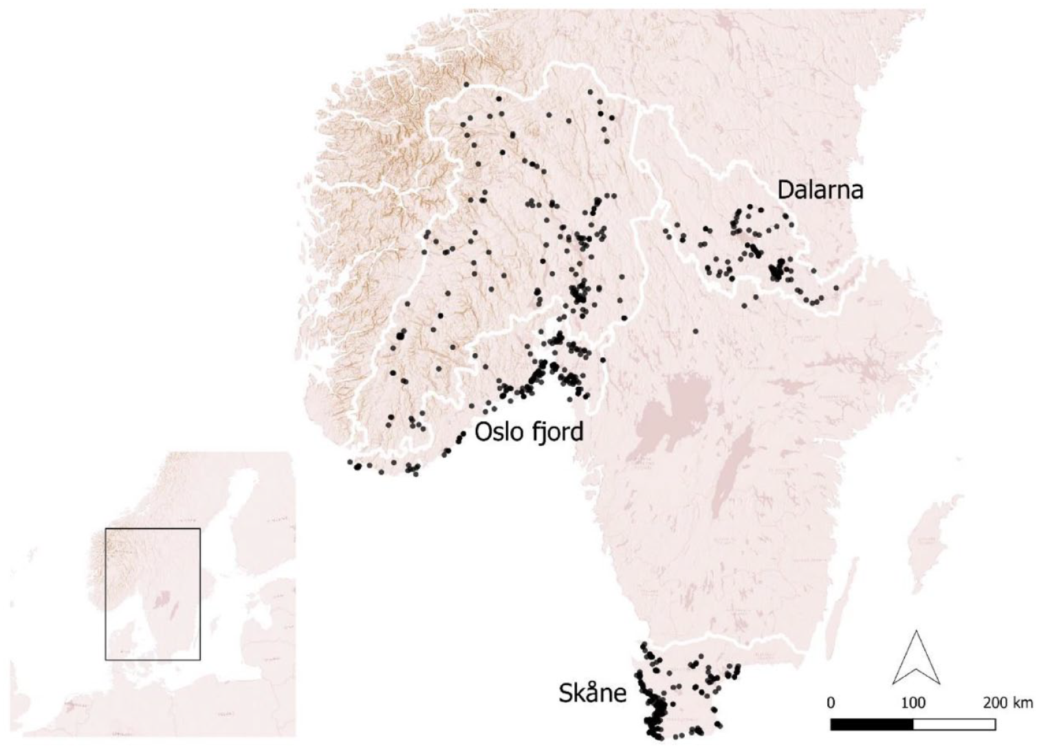
Map showing inland and coastal study regions (white outline) of Norway and Sweden, as well as locations for the 4016 radiocarbon dates (black points) used in this analysis.

Our research area in Norway spans latitudes 57.9°–62.3°N (Figure 1) and it is also divided into (1) inland, which includes highland/mountain regions, and (2) coastal areas. The division into “coastal” and “inland” regions is based on their distinct climates and topography. The coastal region experiences a humid climate with mild winters; the most fertile areas are found along the Oslo fjord and inland Lake Mjøsa. The inland experiences a rain shadow effect that limits rainfall and produces significant temperature fluctuations between seasons. The lower-lying parts of the inland consist of dense forests and bogs, while the elevated areas include alpine and sub-alpine regions. The inland provided valuable resources during the Iron Age for pastures, hunting, trapping, and iron production, while sufficient arable land was still essential for farming (Holm et al., 2005; Loftsgarden, 2019; Svensson, 1998).

Methods

The iLOVECLIM model

iLOVECLIM (hereafter version 1.1) (Quiquet et al., 2018) is a three-dimensional model classified under Earth system models of intermediate complexity, EMICs (Claussen et al., 2002), due to its simplified representation of the atmosphere relative to Global Circulation Models (GCMs). As a result of its efficient description of climate dynamics, iLOVECLIM is substantially faster than coupled GCMs. (Goosse et al., 2010; Kitover et al., 2015). iLOVECLIM is a code fork of the LOVECLIM 1.2 model (Goosse et al., 2010) and shares the main climate system components. The version applied in our study includes the atmospheric model ECBilt (Opsteegh et al., 1998), Coupled Large-scale Ice-Ocean model CLIO (Goosse and Fichefet, 1999), and the terrestrial vegetation and carbon allocation model VECODE (Brovkin et al., 1997). The reader is referred to the supplementary information for more details about the components of the model and how it has been used previously to simulate some past climate periods.

In this study, we utilized a dynamically downscaled version of the coupled iLOVECLIM model to enhance its spatial resolution for temperature and precipitation (Quiquet et al., 2018). This downscaling procedure allowed for a higher spatial variability in simulating the Holocene climate in Europe, leading to better alignment with proxy-based reconstructions compared to the standard model (Arthur et al., 2023). For a more detailed explanation of the physics applied to the dynamical downscaling in the model, please refer to (Quiquet et al., 2018).

Set-up and simulations

We conducted ensemble experiments, both with and without volcanic forcings, using the iLOVECLIM-1.1 model (Quiquet et al., 2018) to simulate the evolution of the climate from 1 to 1000 AD. We forced the simulations with orbital forcings to represent variations in eccentricity, obliquity, and precession (Berger, 1978) and atmospheric trace gas concentrations of CO₂, CH₄, and N₂O (Raynaud et al., 2000). Constant ice sheet configurations were prescribed for the experiments. Four different simulation groups were performed, referred to as VOLC_50, VOLC_1000, NOVOLC_50, and NOVOLC_1000, and each consisting of 10 ensemble members. For instance, VOLC_50 consists of 10 equilibrium experiments which were run for 50 years with the same forcings at 1 AD, including volcanic eruptions but different initial conditions. Each initial condition of the simulation is derived from the previous ensemble run. The NOVOLC_50 simulation shares the same setup as VOLC_50 but excludes volcanic eruptions and uses different initial conditions. VOLC_50 and NOVOLC_50 were run to establish distinct climate states that serve as the initial conditions for our 10 ensemble transient simulations (VOLC_1000 and NOVOLC_1000). VOLC_1000 is a transient experiment with volcanic eruptions applied from 1 to 1000 AD (1000-year run) using the same climate forcings for all 10 ensemble members but with different initial conditions derived from the VOLC_50 simulations (see Supplementary Information, Table S1, for specific volcanic forcings applied for 536/540 AD). On the other hand, NOVOLC_1000 is a transient experiment without volcanic eruptions applied over the same period, with the same climate forcings for all 10 ensemble members but with different initial conditions derived from the NOVOLC_50 simulations.

To account for uncertainties associated with internal climate variability due to the chaotic nature of the climate system, we employed a 10-member ensemble simulation. Each member has identical atmospheric physics, dynamics, parameters, and forcings but starts with different initial conditions, resulting in diverse evolutions. The range covered by the 10 members provides an estimate of the internal variability. However, the ensemble mean represents the average response to the volcanic forcing, as the averaging over the ten members effectively mitigates the individual members’ noise and reveals a common signal among them. We present the results of the volcanic eruption simulations as anomalies with respect to the experiment without volcanic eruptions. This approach highlights the impact of volcanism on the climate in our regions of interest.

Volcanic forcings

The volcanic forcing set named eVolv2k, used for the 536 and 540 AD eruptions in VOLC_1000, is described in detail elsewhere (Jungclaus et al., 2017; Sigl et al., 2015; Toohey and Sigl, 2017). The eVolv2k database includes estimates of the magnitudes of the volcanic stratospheric sulfur injection (VSSI) events and their source of eruption (latitudes) from 500 BCE to 1900 CE, based on the measurements from the Antarctica and Greenland ice cores. In the iLOVECLIM model, the stratospheric sulfate loading is derived from ice core deposition using the model from Gao et al. (2008). The sulfate loadings are then converted into an equivalent total solar irradiance (TSI) anomaly through the aerosol optical depth (AOD) by a linear scaling (Mairesse, 2013), where volcanism is considered a negative anomaly of TSI (W/m²) in the iLOVECLIM model (Mairesse, 2013).

In the model, volcanic forcing can be applied in four different latitudinal bands: extra-tropical and tropical bands, separately in both hemispheres. For this study, we focus on the double eruption of 536/540 AD. The 536 AD eruption is assigned to the Northern Hemisphere extra-tropical band, and the 540 AD eruption to the tropical band in the model (Toohey and Sigl, 2017). The volcanic forcings for other periods in the simulations (1–1000 AD without 536/540) are prescribed in the iLOVECLIM model from Goosse et al. (2010).

Spatial-temporal analysis of archeological radiocarbon (¹⁴C) data

Using summed probability distributions (SPD) of radiocarbon dates to study large-scale demographic and environmental processes is an established method across various disciplines. It has evolved from the time-series analysis methods of researchers like Deacon (1974) and Geyh (1980), who used radiocarbon dates as proxies for demographic and environmental change, respectively (see Carleton and Groucutt (2021 for a history of the approach’s development). Following these earlier research contributions, Rick’s “Dates as Data” (Rick, 1987), emerged as a pivotal work, frequently referenced for using radiocarbon dating as proxies to explore temporal developments in human activity.

In the past three decades, significant advancements in calibration programs and computing technology have enhanced the utilization of SPDs of radiocarbon dates. However, longstanding debate about the reliability of the technique remains (Brown, 2015; Carleton and Groucutt, 2021; Williams, 2012). Critics contend that relying on a qualitative assessment or “eyeballing” of SPDs lacks statistical rigor and introduces subjective inferences (Crema, 2022). They argue that such approaches may mask systematic and random errors, including issues related to sample size, sampling intensity bias, taphonomic loss, calibration, and measurement error, potentially leading to misinterpretations (Crema, 2022). To address imperfect data in archeology and palaeosciene, computational statistical analysis has emerged as a valuable approach to enhance the robustness of interpretations and conclusions drawn from radiocarbon date distributions (Crema, 2022; Shennan et al., 2013).

For our analyses, we employ a quantitative approach using the rcarbon package (version 1.5.0) from the R programing environment. This package offers a statistical framework for the aggregate analysis of ¹⁴C data, accounting for systematic and random errors inherent in ¹⁴C analysis through its provided functions (Crema and Bevan, 2021). We compared regional summed probability distributions (SPDs) against a logistical growth model as well as compared regional and categorized land use SPDs against one another (see Crema, 2022 for a detailed description). This approach, following methods from previous works (Brown and Crema, 2021; Crema et al., 2016, 2017; Riris and Arroyo-Kalin, 2019; Shennan et al., 2013; Timpson et al., 2014), requires first calibrating and binning ¹⁴C samples based on temporal proximity (h = 50; see Fig. S15 for sensitivity analysis). Binning attempts controls for sampling intensity bias (Crema, 2022). Next, we generated normalized SPDs from the observed data, and fit them to a logistical growth model and conducted mark permutation tests between our regions and land uses. Null hypothesis testing takes into account calibration effects by creating an expected range of SPDs, or a 95% critical envelope, through the Monte-Carlo method (nsim = 1000) that addresses sampling errors (Crema and Bevan, 2021).

Our spatial analysis, also utilized a permutation test, sptest(), from the rcarbon package, where spatial positions of sites are shuffled randomly, and departures from the permuted null are calculated with p-values and false discovery rates (q-values) to assess the significance of these departures (Brown and Crema, 2021; Crema et al., 2017; Crema and Bevan, 2021). Our spatial analysis was based on a bandwidth of 25 km, comparable to the resolution of the iLOVECLIM climate simulation.

Archeological radiocarbon ¹⁴C datasets

Throughout our analysis, we reuse existing data and utilize open-source software, highlighting the significance of and advocating for FAIR data practices (e.g. Wilkinson et al., 2016). Through the diligent efforts of previous researchers, we gained to access rich ¹⁴C databases in our study regions (see Acknowledgments) and reoriented our analyses to compare the effects of the volcanic event and the so-called Fimbulwinter on topographically and economically diverse regions of inland and coastal Sweden and Norway. This approach facilitates comparative analysis, shedding light on how environmental impacts may have influenced regional land use.

These datasets contain over 12,238 dated records spanning most of the Holocene. However, due to our study’s specific focus on the 536/540 volcanic event, we restricted our examination to the first millenium AD, enabling the establishment of demographic and land use patterns in the region across three climatic transitions: (1) before the volcanic event, (2) during the Fimbulwinter, and (3) the subsequent climate recovery period. This filtering process resulted in a dataset of 4016 Scandinavian records (see Figure 1; Norway n = 1555, Sweden n = 2461, sites n = 1894). With our substantial sample size and a focus on general trends, we have confidence that the impact of any individual source of error is minimal and does not significantly affect our research outcomes (Riris and Arroyo-Kalin, 2019; Shennan et al., 2013; Timpson et al., 2014).

Land use categorization

Our research aims to understand past human responses to environmental risks through not only the spatiotemporal analysis of population trends, but also categories of land use. Our extensive ¹⁴C datasets, we have been able to assign each ¹⁴C record in our database to a general land use category that considers the context of artifacts, features, and site type associated with the sample. As land use activities vary greatly over time and space, our categorizations are intentionally broad and high-level and aim to represent cultural changes and adaptations to external factors. Grouping the data into inclusive categories helps reduce noise in the material and facilitates our exploration of general patterns in response to climatic events. Despite our extensive dataset, challenges arise due to the disproportionate representation of certain sites or structures in the records. For instance, remains from iron production in specific inland regions of Norway between AD 600 and 700 to 1350 and cooking pits, particularly abundant between AD 200 and 600, may skew the data due to their visibility and higher dating frequency (Gundersen et al., 2019; Larsen, 2009; Loftsgarden, 2020; Rundberget, 2013). The land use categories are adapted from Hatlestad et al. (2021) and are informed by the data discussion on cultural change in the categories and contextual associations are as follows:

• Settlement: Postholes, hearths, cooking pits, foundations, cellar pits, pit houses, longhouses, floor layers, remnant fields, urban plots, and ovens are examples of the features that were, when found in combination, interpreted as settlements in study area archeological site reports;

• Iron production: Bloomeries, charcoal production sites, slag, roasting features, forging pits, casting pits;

• Agriculture: cultivation terraces, clearance cairns, fences, enclosures, irrigation ditches, and flax processing sites as agriculture features;

• Hunting: pitfall traps, high altitude/melting glacier hunting finds

• Other: all other dates that did not meet the criteria for the above categories

Results

Climate results

Simulated ensemble mean temperature change during the volcanic period (536–541 AD) relative to the NOVOLC_1000 experiment show pronounced cooling in Scandinavia and the whole of Europe (Figure 2b), with a maximum ensemble mean cooling of −1.1°C reached after the eruption. The inland and coastal areas of Norway, Dalarna, and southern Sweden exhibit temperature change of up to –1°C relative to the simulation without volcanic forcing (Figure 2b). The ensemble mean represents the average response to the volcanic forcing, effectively canceling out the noise of the individual ensemble members; the “real” climate signal observed in proxy data reflects both internal variability and external forcings like volcanic eruptions. Consequently, the ensemble mean representing the forced response should not be the sole focus when comparing model results with proxy data.

Figure 2.

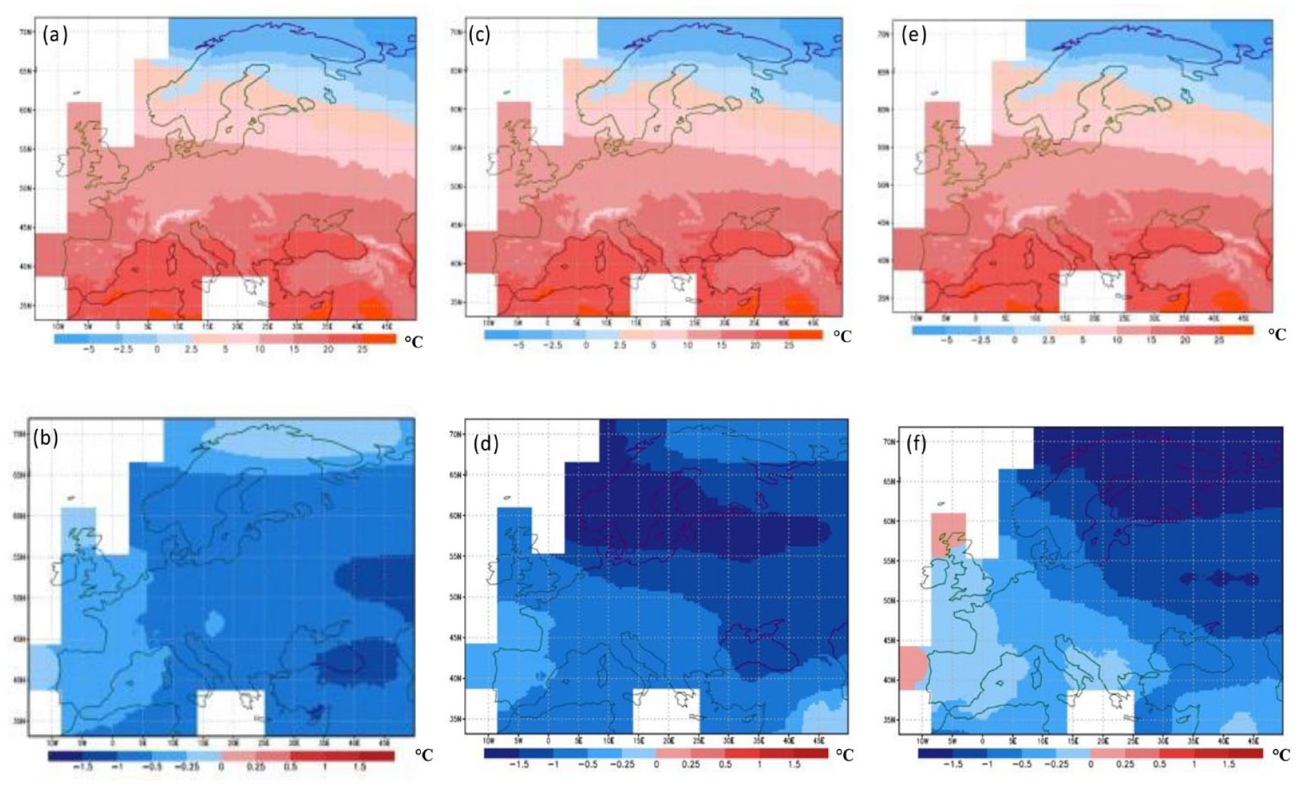
(a) Shows the ensemble mean temperature (all 10 ensemble members) simulated without volcanic eruption, averaged from 1 to 1000 AD as reference period; (b) Ensemble mean temperature change during the volcanic eruption (536–541 AD) relative to the ensemble mean temperature without volcanic eruption While (c and e) show ensemble member 1 and 7 temperatures respectively without volcanic eruption, averaged from 1 to 1000 AD as reference period. (d and f) show ensemble member 1 and 7 temperature change respectively, during the volcanic eruption (536–541 AD) relative to ensemble member 1 and 7 simulated without volcanic eruption (i.e. the reference period).

Consistency between the model and data implies that the proxy signal should lie within the simulated climate range of the ensemble set, which includes both the forced response and internal variability (Goosse and Renssen, 2004). In this context, the climatic signal observed in proxies is similar to the results of a specific ensemble member. To assess the full range of climate responses, we consider two ensemble members (1 and 7) that exhibit relatively large climate change during the volcanic forcing. Figure 2d and f show temperature changes for the double eruption event relative to NOVOLC_1000 for ensemble members 1 and 7, respectively.

Ensemble member 1 indicates temperature decreased by more than −1.5°C during the eruption in most regions of Norway and Sweden. For ensemble member 7, temperature anomalies fall below −1.5°C, with inland Norway and central Sweden experiencing changes between (–1°C and −1.5°C) relative to NOVOLC_1000. In southern Norway and Sweden, temperature changes ranged from −0.25°C to −0.5°C for ensemble member 7 (Figure 2f).

Precipitation also responded to the significant explosive volcanic eruption with a decrease in most European regions. Figure 3a shows the model ensemble mean spatial patterns of precipitation averaged from 1 to 1000 AD (without volcanic eruption), while Figure 3b shows the ensemble mean change averaged from the eruption period (536–541 AD) relative to Figure 3a. The ensemble model indicates a clear decrease in precipitation following volcanic eruptions, particularly in Scandinavia, where negative change of up to −25 mm/year are observed. Some areas in Norway have precipitation change ranging from −25 to −50 mm/year, indicating dryness post-eruption. This reduction in precipitation is attributed to a decrease in short-wave radiation reaching the surface due to the eruption (Figure S3: Supplemental information), which leads to reduced evaporation and atmospheric stabilization (Cao et al., 2012). Additionally, a cooler atmosphere undergoes less radiative cooling to space, allowing less condensation and precipitation (Allen and Ingram, 2002; O’Gorman et al., 2012).

Figure 3.

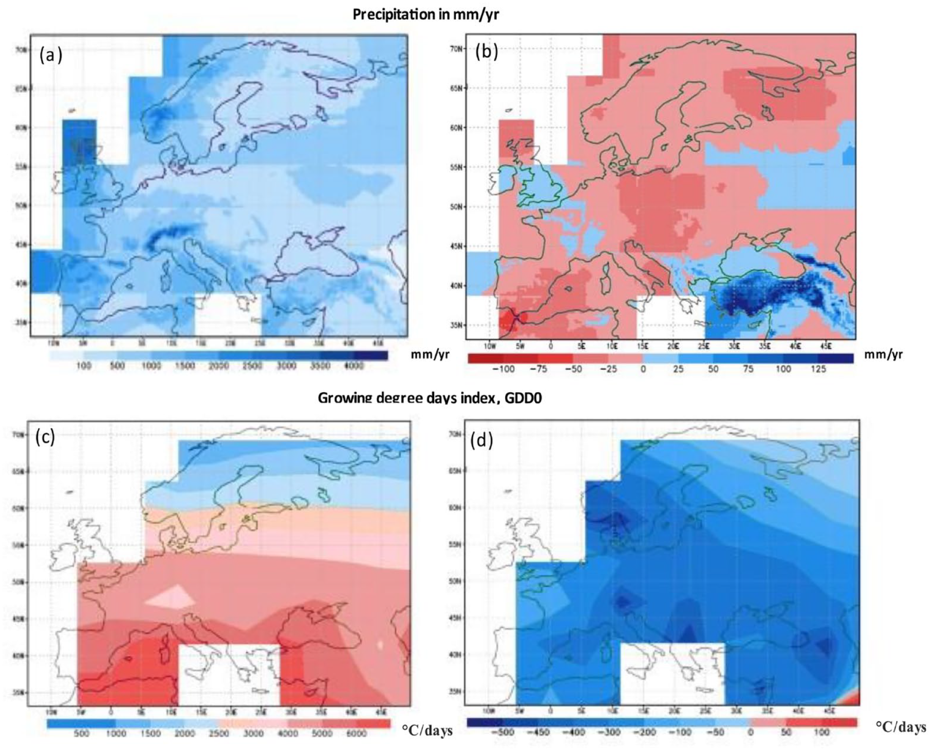
Showing (a) Ensemble mean precipitation simulated without volcanic eruption, averaged from 1 to 1000 AD (NOVOLC_1000) as reference period; (b) Ensemble mean precipitation change during the volcanic eruption (536–541 AD) relative to NOVOLC_1000; (c) Growing Degree Days index (GDD0) simulated without volcanic eruption, averaged from 1 to 600 AD and (d) Growing Degree Days index change during the eruption period (536–541 AD) relative to the GDD0 without volcanic eruption expressed as °C-days.

Volcanic response in different regions

Figure 4 shows the temperature evolution in our selected study regions, including all 10 ensemble members and their ensemble mean for the model simulations from 500 to 600 AD with volcanic eruption. In Dalarna, the results indicate an immediate cooling at 537 and 541 AD after the eruption, with the mean ensemble temperature declining from 5.2°C to 4.5°C and 4.1°C, respectively, following the eruption at 536. The model ensemble means change at 537 AD was −1.2°C and −1.6°C at 541 AD compared to the no volcanic ensemble mean for this inland Sweden region (Figure S2: Figure in Supplemental Material). The temperatures started to rise again after the eruption in 543 AD.

Figure 4.

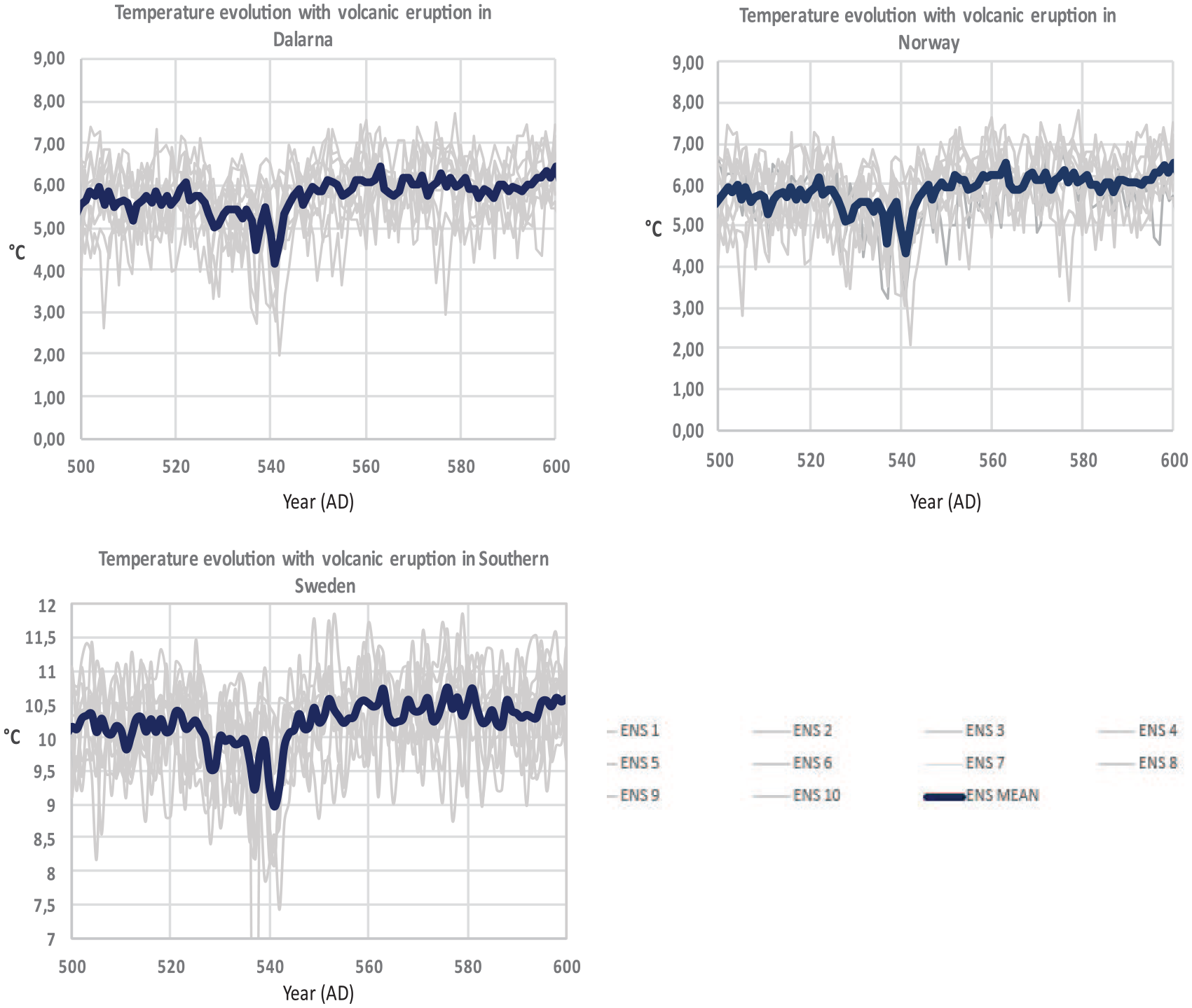
Time series of the temperature ensemble runs simulated by the climate model (iLOVECLIM) with volcanic eruption applied in our study regions (Dalarna, Norway, and South Sweden). All the 10 ensemble members are shown in gray with the ensemble mean in deep blue color.

The southern Sweden (Coastal) study region (Figure 4) also shows a temperature decrease following a pattern similar to Dalarna but with different changes and recovery periods in response to the volcanic eruption. The volcanic signals are significant and clearly shown, with maximum cooling observed in the first (537 AD) and second year (541 AD) after the eruption, followed by a gradual rise after 543 AD for over 30 years.

We utilized a student t-test to establish the statistical significance of the volcanic eruption’s impact on the ensemble simulations. By comparing the change in temperature of the ensemble mean during the volcanic period (536–541 AD) to the average ensemble mean temperature without the volcanic eruption period (536–541 AD) for all study regions, we determined p-values. Southern Sweden showed p-values below 0.05 (Table S2, Supplemental Material), indicating a significant cooling at 95%. Norway and Dalarna had p-values below 0.1, indicating substantial cooling at 90%. This statistical test is crucial to validate the confidence in our results, Our test gives us confidence than the volcanic eruption during the 536–541 AD had an impact in the regions we studied in Scandinavia, showing that the change in temperature between the two experiments was due to the impact of the volcanic forcings prescribed in the simulations.

Growing degree days (GDD0)

The simulated ensemble mean temperature changes are similar across the study areas after the 536 and 540 eruptions. However, the impact of climate variability on society and society’s response depends on its effect on agriculture in different regions. To understand agricultural vulnerability, we analyzed changes in simulated growing degree days (GDD0), the sum of daily mean temperatures above a given threshold (in our case, 0°C) to provide GDD0 during the growing season.

The simulated GDD0 index changes during the eruption (relative to NOVOLC_1000) showed a substantial reduction in plant growing conditions in Scandinavia and the rest of Europe (Figure 3d). The GDD0 anomalies were between −400 and −500 degree days in the coastal regions of Norway and Sweden, while the GDD0 anomalies of Sweden and Norway’s inland were between −200 and −400 degree days, which indicates a larger limiting impact on plant growing conditions on the coast than the inland.

Figure 5 displays localized Scandinavian temporal trends in the growing degree days index following the volcanic eruption. The results show southern Sweden experienced the most negligible impact on the growing season compared to the inland areas in Norway and Dalarna, with coastal Norway having the most drop in GDD0 during the eruption period.

Figure 5.

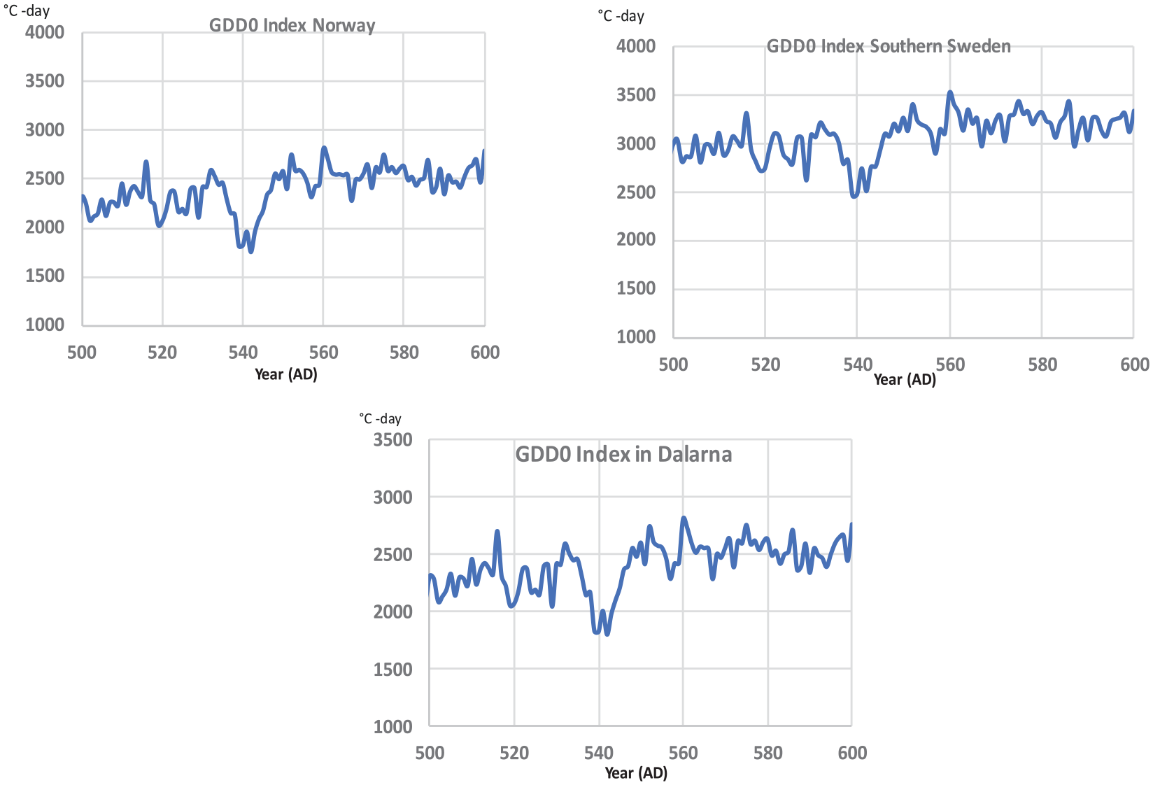
Time series of the Growing Degree Days index simulated with volcanic eruption applied in the iLOVECLIM model in our study regions (Dalarna, Norway, and Southern Sweden).

The trends in GDD0 follow similar patterns in all regions, but the degree index and percentage change magnitude differ. In Dalarna, GDD0 decreased by approximately 27% during the eruption but later recovered (Figure 5). Before the eruption, in 535 AD, GDD0 was around 2452°C-days but declined to 2138°C-days in 537 AD, then 1818°C-days to 540 AD, with its lowest level of 1794°C-days occurring in 542 AD. However, the GDD0 started rising again in 543 AD, reaching a peak of 2803°C-days in 560 AD (Figure 5). Norway experienced about 29% reduction in the length of the growing season after the eruption, with GDD0 declining from 2461°C-days (535 AD) to 1752°C-days (542 AD) (Figure 8). Southern Sweden also had a 20% reduction in growing degree days, decreasing from 3101 (535 AD) to 2477°C-days (540 AD). Coastal Norway showed the most significant reduction during the event, with a drop of almost 500°C-days, while the inland experienced a reduction of 400°C-days as shown in (Figure 3d).

Null model hypothesis testing of 14C datasets

The logistical growth model analysis of our data set as whole reveals a significant negative departure from the null occurring just after the 536/540 AD event (Figure 6). The observed SPD’s lack of fit within much of the 95% confidence envelope, coupled with a global p-value of 0.001, suggests an effect on demographic growth at this time. Similar significant negative deviations after the 536/540 AD event are observed in coastal and inland Sweden. However, while growth in these regions falls below the null’s expectations, the observed SPDs still reflect increasing growth. In both of Norway’s regions, the observed SPD begins a downward trend close to the 536/540 AD eruptions, but there is an approximate 10 to 20-year lag before a significant negative deviation from the null.

Figure 6.

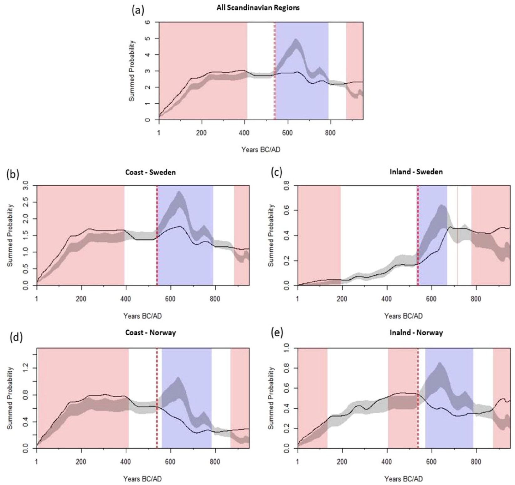
Logistical growth models for (a) all Scandinavian regions (n_dates = 4016, n_sites = 1898, n_bins = 2583, p-value = 0.001); (b) Coastal Sweden (n_dates = 2093, n_sites = 755, n_bins = 1389, p-value = 0.001); (c) Inland Sweden (n_dates = 368, n_sites = 280, n_bins = 254, p-value = 0.001); (d) Coastal Norway (n_dates = 879, n_sites = 435, n_bins = 508, p-value = 0.001); (e) Inland Norway (n_dates = 676, n_sites = 428, n_bins = 432, p-value = 0.001). Gray area represents the 95% confidence envelope of the fitted logistical growth model. Black line represents the observed SPD with red areas showing periods exceeding the expected growth and blue areas showing periods below the expected growth. The dashed red line represents the 536/540 AD event.

Mark permutation test

The initial permutation test results (Figure 7) reveal significant divergences in demographic patterns between Norway and Sweden in the first millenium AD (Crema and Bevan, 2021). In Sweden’s inland region (p-value = 0.001), significant deviations below the permuted null persist until shortly after the volcanic event. Following 536/540 AD, regional growth recovers, meeting the confidence envelope before exceeding expectations around 650 AD. Meanwhile, coastal Sweden’s observed SPD (p-value = 0.008) closely adheres to the confidence envelope but trends upwards just before the Fimbulwinter, deviating positively from the null approximately 50 years after the event.

Figure 7.

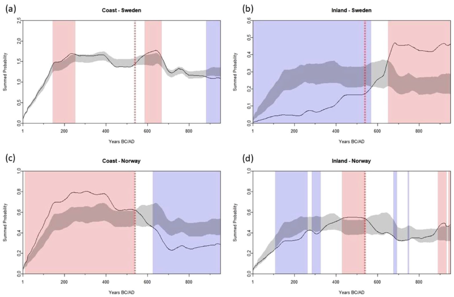
Permutation test comparing (a) Coastal Sweden (n_dates = 2093, n_sites = 755, n_bins = 1389, p-value = 0.001); (b) Inland Sweden (n_dates = 368, n_sites = 280, n_bins = 254, p-value = 0.001); (c) Coastal Norway (n_dates = 879, n_sites = 435, n_bins = 508, p-value = 0.001); (d) Inland Norway (n_dates = 676, n_sites = 428, n_bins = 432, p-value = 0.001). Gray area represents the 95% confidence envelope of the permutation null model (i.e. where the distribution is calculated from a rearrangement or permutation of the observed ¹⁴C records). Black line represents the observed SPD with red areas showing periods exceeding the expected growth and blue areas showing periods below. The dashed red line represents the 536/540 AD event.

Conversely, Norway’s regions positively deviate from the null leading up to the 536/540 eruptions, but then experience a decline. This reduction may have started before the volcanic event (Figure 7), raising the curiosity as to whether the eruption triggered a demographic and social restructuring or intensified an ongoing societal transformation. These results will be further discussing in the following discussion section.

Spatial permutation tests

Using the spatial permutation method provided by the rcarbon package, we analyzed the geographical intensity of population and land use activity in the Scandinavian region over two centuries (450–650 AD) (see SI and Crema et al., 2017 for an in-depth explanation of this approach; Brown and Crema, 2021; Crema et al., 2017). Our findings indicate an increased dependence on the inland regions of Sweden and Norway, a substantial decline in the Norwegian coastal area, a heterogenous results for the southern coast of Sweden (Figure 8; Figure S5–S9, Supplemental Material).

Figure 8.

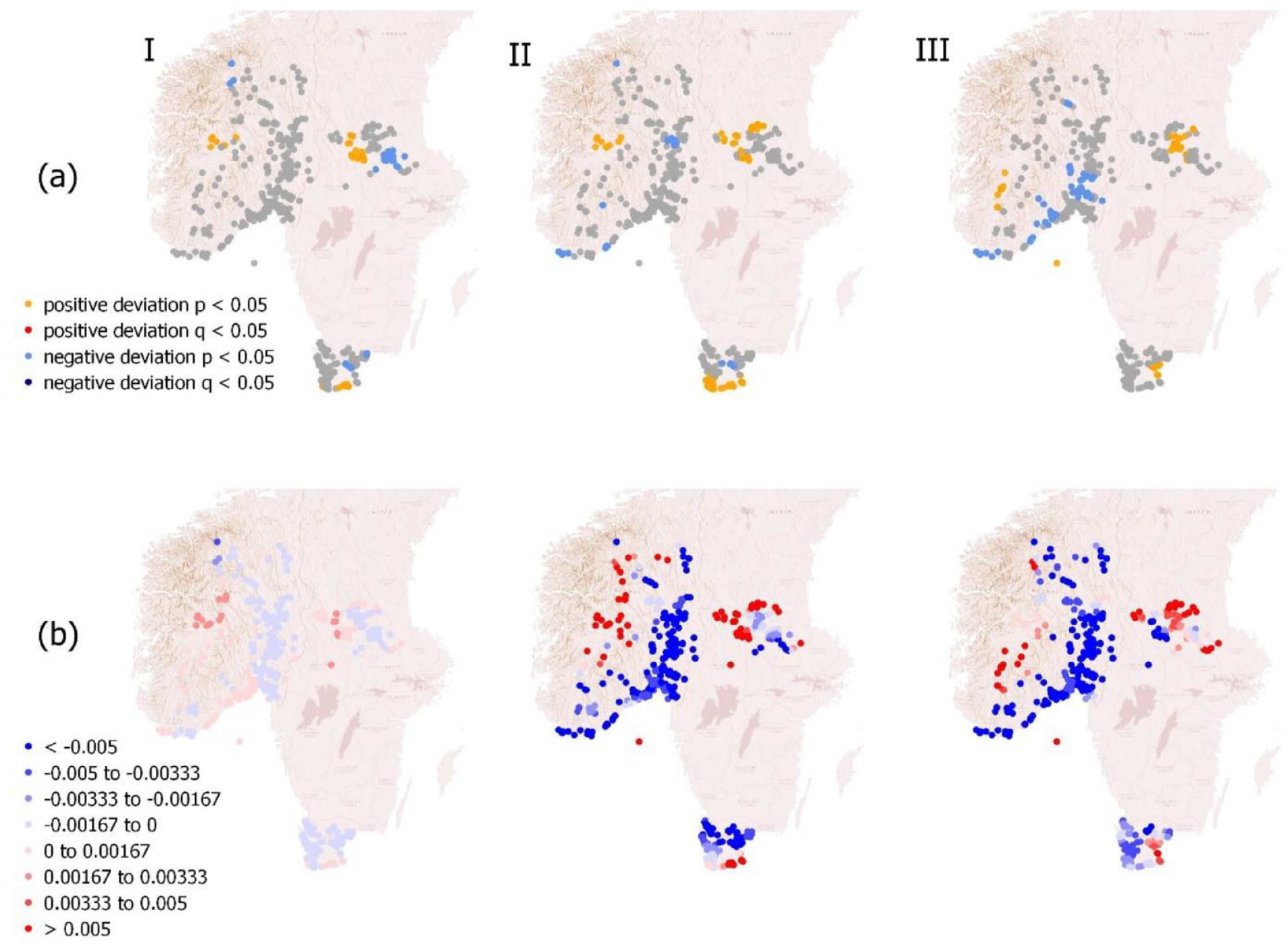
(a) rcarbon sptest () (i.e. spatial permutation test) for all radiocarbon dated sites in Scandinavian study regions across three transitions: (I) 450–500 to 500–550 AD, (II) 500–550 to 550–600 AD, (III) 550–600 to 650 AD, depicting “hot and cold” spots of growth with p-value and q-value deviations. (b) Local geometric growth rates across transitions I-III.

The results for the Swedish inland align with our previous permutation analysis, showing a significant positive deviation after the Fimbulwinter. However, this spatial permutation test revealed a Norwegian inland hotspot not detected in the earlier analysis, highlighting how region-specific nuances can be obscured with a solely temporal permutation approach (Figure 8a).

Across the 200-year time block, pronounced growth is observed in the inland regions and the southernmost tip of Sweden, while Norway’s Oslo fjord coastal region shows decline (Figure 8). Southern Sweden’s coast displays variation, with the northern portion experiencing a decline in growth and less fluctuation at the southernmost border. In the third transition, a geographic shift in land use intensity is evident, with an expansion southward in inland Norway and eastward in inland Sweden, possibly indicating recovery and a return to areas previously utilized before the Fimbulwinter (Figure 8b).

Land use tests

We analyzed regional land utilization to extend the investigation of the overarching demographic patterns, which had previously suggested an increased dependence on the boreal inland following the 536/540 AD event. Thus, we employed a spatial permutation test to examine specific spatial alterations in land use over a 200-year timeframe, which revealed notable changes in several land use categories (see Figure S5–S9, Supplemental Material).

During the three transitions, settlement activity deviated negatively, especially along the Norwegian coast (Figure S5a, Supplemental Material). However, southern Sweden exhibited only a slight decline in growth rates (Figure S5b) across transitions I–III, still surpassing the expectations of the null model (Figure S5a). Meanwhile, the inland region of Norway experienced pockets of considerable positive settlement growth, exceeding the expectations of the null model, whereas settlement in inland Sweden only trended positively in transition III.

Limited ¹⁴C records hindered a prominent agricultural signal, but local growth rates indicate increased activity around the Oslo fjord and inland Sweden in the first two transitions (Figure S7a). Transition III witnessed a decline in coastal growth rates and Sweden’s inland region exhibited heterogeneity (Figure S7b).

Similarly, our datasets contained limited hunting records for these periods, but hunting appeared more prevalent in the inland regions, with Norway’s hunting declining across transitions and Sweden’s increasing (Figure S8).

Iron production significantly grew in the inland areas of Norway and Sweden over the transitions (Figure S6b). Inland Norway presents as an iron production hotspot during the first two transitions, while Sweden’s iron production rising notably during transition II, or the fimbulwinter event period, and thereafter (Figure S6a). Moreover, as observed in the overall demographic activity, the same geographical shift eastward in inland Sweden is reflected in the third transition, or climate recovery period (Figure S6b).

Discussion

Summary of results

The iLOVECLIM climate simulations reveal distinct patterns of temperature, precipitation and GDD changes during the volcanic period, with variations observed between our coastal and inland regions. Temperature results show an overall regional decrease in mean ensemble (−1°C), yet the inland areas see a larger reduction in temperature, with ensemble 7 yielding a more regionally varied difference in temperature (−1°C to −1.5°C inland and −0.25°C to − 0.5°C coastally) compared to the mean and ensemble 1 (−1.5°C). Precipitation results are generally homogenous between regions, with negative changes of up to −25 mm/year observed and a few areas in Norway with changes of up to −50 mm/year. Simulations of GDD for regional coastal areas show changes between −400 and −500 degrees days, while the inland regions changes were between −200 and −400 degree days.

Our spatial-temporal analysis of ¹⁴C archeological data also reveals distinct regional patterns in the demographic chronology and land use activities surrounding the 536/540 event. All regions negatively deviate from the logistical null either during or closely after the volcanic event. Notably, the Swedish regions’ observed SPDs trend positively around 536/540 AD, while Norway’s observed SPDs trend negatively. However, results from the mark permutation test somewhat alter these findings, as significant deviations in the demographics of coastal Norway and both inland regions end just before or around 536/540 AD (Figure 7b–d). Additionally, the coastal Sweden region shows significant deviations approximately 50 years after the event and then trends positively (Figure 7a). The spatial permutations findings indicate an increased spatial intensity occurring in the inland regions of Sweden and Norway, a substantial decline in the Norwegian coastal area, a heterogenous results for the southern coast of Sweden during the modeled volcanic event period (500–550 to 550–600 AD) (Figures S5–S9).

Moreover, the land use mark permutation tests highlight regional variations occurring around Transition II (500–550 to 550–600 AD). Coastal Norway emerges as a cold spot for settlement, with specific local growth rates indicating declines in settlement and iron production, an uptick in agriculture, and a decline in the other category sites. Inland Norway maintains two small hotspots of settlement before, during, and after the volcanic event, with local growth rates increasing during transition II. Similarly, the region experiences positive trends in iron production during Transition II. Coastal Sweden is a minor hotspot for settlement during Transition II, mixed cold and hotspots for agriculture and hunting, and declining sites in the “other” category. Inland Sweden also emerges as a minor hotspot for settlement, becoming an iron production hotspot after the volcanic event (550–600 to 600–650 AD). However, local growth rates in this region indicate an increase in iron production, agriculture, hunting, and other activities during Transition II.

Regional societal response to the 536/540 AD volcanic event

During the volcanic event, Norway’s coast experienced the largest decrease in GDD0 among all four regions, reaching −500-degree days (see Figure 3d). This decline in GDD0 can be attributed to a combination of temperature and precipitation factors, although individually, these variable changes were not as drastic as compared to other regions. The significant decrease in GDD0 suggests that crop growth and production were more severely affected in this region, particularly in the Oslo fjord area, which relied more heavily on domestic crops compared to the mixed farming inland areas (Bevan et al., 2017; Eriksson et al., 2021; see Figures 3d and 5, Figure S7). The GDD0 values can be compared to specific crops relevant to the study area (Table S2). Figure 5 indicates that the volcanic eruption may have limited wheat and buckwheat growth but not barley, which dominated crops in Norway and Sweden during the first millenium BC (Widgren and Pedersen, 2011). The ¹⁴C land use tests reveal a slight increasing trend in agriculture leading up to and during the 536/540 AD event, followed by a decline during the climate recovery period, raising questions about the lag time between a climate event and societal change, and the significance of crop diversification as a coping strategy.

The trend in the archeological ¹⁴C results for Norway’s coast during the same period indicates general decreased spatial-temporal intensity in demography and land use, suggesting region’s specific environmental risks, such as its latitude and topography, may have pushed it past a critical threshold, contributing to unavoidable activity declines. However, our land use analysis of the region shows a reduction in the diversity of activities had begun prior to the Fimbulwinter period (Figures S10, S13), possibly affecting the region’s ability to quickly adapt to the 536/540 AD event. Additionally, the evidence of prior land use change suggests that social influences, possibly the Migration period upheaval (400–800 AD), were already affecting the region before 536/540 AD. The volcanic event may have augmented this ongoing change (Eriksson et al., 2021; Gjerpe, 2017; Iversen, 2016; Loftsgarden and Solheim, 2023).

Norway’s inland, also experienced quite drastic declines in GDD0 (−400-degree days), temperature (−1 to −1.5°C) and precipitation (up to −50 mm/year). However, this region’s permutation results show hotspots of demographic intensity before, during and after the 536/540 event. ¹⁴C records of land use also present as more robustly diverse, both in intensity and in number, than its coastal counterpart prior to the volcanic event (Figure S10, S14). Specifically, there is an increase in iron production after the volcanic event and agricultural activity remains stable for a period. The trends observed imply that in challenging environments, where diverse economic strategies like iron production and agri-pastoral farming are necessary, trade continued to be a valuable adaptive response to uncertainties. These economic pursuits provided communities with added resilience, ensuring their ability to cope with sudden environmental adversities.

The iLOVECLIM model simulated similar climate effects of the volcanic event on coastal Sweden as coastal Norway, presenting decreasing temperatures (−0.25°C to − 0.5°C), precipitation (−25 mm/year) and GDD0 (−400-degree days). This implies a potential impact on agricultural productivity due to a shortened growing season, with increased frost days and higher likelihood of drought. Though similar climatic variability occurs here as on the Norwegian coast, demographic and land use trends present as generally stable and within expected critical envelope ranges (S10, S11) in the face of the volcanic event. Unlike the Norwegian coast, the land use intensity levels in coastal Sweden prior to the volcanic event were generally stable and, in some cases, even displayed positive trends. This finding reinforces the idea that stability is resilient and difficult to disrupt. It also highlights the importance of creating diverse resources and strategies to withstand and adapt to abrupt events effectively.

Inland Sweden experienced a relatively minimal climatological impact during the 536/540 AD event, with decreases of approximately −200-degree days in GDD0, −1.2°C and −1.6°C in temperature, and −0.25 mm/year in precipitation compared to other regions. Despite this, the spatial-temporal analysis of inland Sweden’s ¹⁴C records shows some degree of growth across all five land-use categories in the aftermath of the volcanic eruption (Figures S10, S12). The region’s unique geographical location, possible favorable microclimates, diversified land uses, and the creation of new grazing space for livestock resulting from forest clearance for iron production likely preconditioned the area for success during the Fimbulwinter (Eriksson et al., 2021; Eriksson, 2023; Hatlestad et al., 2021; Löwenborg, 2023; Oinonen et al., 2020). Just like in inland Norway, the fact that iron production continued in inland Sweden after the Fimbulwinter indicates that trade remained a viable strategy for coping with environmental risk.

Uncertainties and future extensions

Most climate models confirm cooling effects following Northern Hemisphere volcanic eruptions, aligning with our dynamically downscaled iLOVECLIM model ensemble setup, which reveals surface cooling during the fimbulwinter in Scandinavia. Recent work by van Dijk et al. (2022) utilizing the Max Planck Institute Earth System Model and identical PMIP4 volcanic forcing as our study, demonstrates significant cooling in mean Northern Hemisphere surface climate for up to two decades post the major eruptions of 536, 540, 574, and 626 AD. Earlier research on volcanic eruption effects within the last millenium, such as Timmreck et al. (2009) and Guillet et al. (2020), indicated a decade-long cooling period following exceptionally large eruptions. Notably, Earth System Model simulations around 536 and 540 AD by Toohey et al. (2016), driven by volcanic forcings, displayed Northern Hemisphere mean temperature anomalies exceeding −2°C, implying substantial crop production reductions across Scandinavia. In agreement with the findings of Toohey et al. (2016), iLOVECLIM simulations also demonstrate a decrease in the GDD0 index across our study areas, lending support to the hypothesis linking the mid-sixth-century social crisis to the volcanic eruptions of 536 and 540 AD.

Divergent ¹⁴C results observed in these studies may be influenced by other concurrent factors, such as famine and plague, which themselves may be a cascading result of sudden perturbations that destabilize the climate and further impact a society’s ability to cope (Bondeson and Bondesson, 2014; Harbeck et al., 2013; Iversen, 2016; Solheim and Iversen, 2019). This underscores the complexity of human-environment dynamics. Nevertheless, our comparative analysis provides strong evidence that mid-sixth century societal transformations in our study regions were influenced by the 536/540 AD volcanic event.

Another issue is a lack of terrestrial hunting data for the Norwegian coast, which can be attributed to its marine geography, indicating a greater dependence on aquatic sources. Unfortunately, there are few archeological sites reflecting the exploitation of marine resources. As a result, our understanding of land use diversification opportunities in this area may be skewed.

Consideration of lag time is crucial when comparing the climate and societal records. Changes in human societies do not often present in the archeological record immediately, resulting in a time delay before responses to environmental influences become evident. Several researchers have developed and employed methods to address this issue. The methods used include running significance tests on the correlation between climate events and differences in population development, to identify “trigger” events or measure temporal lags between population decline and change in environmental proxy age depth models (Donges et al., 2016; Siegmund, Siegmund and Donner, 2017; Heitz et al., 2021; Riris and de Souza, 2021; Kim et al., 2021; Kintigh and Ingram, 2018). By considering these lag time factors and employing rigorous statistical methods, researchers can gain a more nuanced understanding of the relationship between climate events and societal changes.

Conclusion

In this study, we conducted a spatial-temporal analysis of ¹⁴C records from Sweden and Norway compared to the downscaled iLOVECLIM climate model. Our results revealed distinct regional capabilities in maintaining land-use systems during the climate variability of the Fimbulwinter. Our investigation concludes with the insights we have gained into our original research questions:

(i) What is the impact of the 536/540 volcanic event on Scandinavian society? Our analysis of the simulated ensemble mean changes and the changes of Ensembles 1 and 7 during the volcanic event, in comparison to the NOVOLC_1000 simulations, revealed abrupt declines in temperature, precipitation, and GDD0 index across all regions during 536 and 540 AD. However, our findings indicate that the impact of these changes varied across regions, with Norway experiencing more severe climatic changes after the event, while Sweden with milder climatic effects, showed fewer indications of societal decline during the same period.

(ii) Can we see evidence for a relationship between patterns of climate and ¹⁴C records? Can we identify the volcanic event as a leading signal to change in the archeological record? Again, we observed pronounced regional disparities in the correlation between the climate simulations and the archeological data. Specifically, while the climate deteriorated in Scandinavia as a whole following the volcanic event, we noted that land use and demography in Sweden remained relatively stable, and even increased in its inland, while the coast of Norway experienced a decline. However, we were not able to definitively identify the 536/540 AD event as a “trigger” for these regions’ changes in demography and land use.

(iii) Did changes in land use or regional spatial intensity occur following the event? If so, what does that indicate about regional capacities to cope with abrupt climate risk?

The spatial permutation tests performed on the ¹⁴C samples allowed us to track regional trends before, during and after the volcanic eruptions. The results reveal that trade, mobility and land use diversification were adaptive societal responses to abrupt environmental risks.

The study enhances our comprehension of the multifaceted relationship between society and the environment and sheds light on the adaptive mechanisms of humans in response to environmental stressors. The outcomes of our investigation emphasize the need for a region-specific approach when evaluating the impact of climate change on societal response. Furthermore, our results point to diversification and mobility as resilient societal adaptations.

Supplemental Material

sj-docx-1-hol-10.1177_09596836231225718 – Supplemental material for The impact of volcanism on Scandinavian climate and human societies during the Holocene: Insights into the Fimbulwinter eruptions (536/540 AD)

Supplemental material, sj-docx-1-hol-10.1177_09596836231225718 for The impact of volcanism on Scandinavian climate and human societies during the Holocene: Insights into the Fimbulwinter eruptions (536/540 AD) by Frank Arthur, Kailin Hatlestad, Karl-Johan Lindholm, Kjetil Loftsgarden, Daniel Löwenborg, Steinar Solheim, Didier M Roche and Hans Renssen in The Holocene

Footnotes

Acknowledgements

We wish to thank our many colleagues for providing their insights, technical assistance and reviews throughout this process, notably Marco Hostettler and Eugene Costello. We are also grateful to Joakim Wehlin for sharing his ¹⁴C database (originally published in Hatlestad et al., 2021) as well as whose database we have accessed thanks to FAIR principles. And many thanks to our co-authors Kjetil Loftsgarden and Steiner Solheim for the reuse of their comprehensive Norwegian ¹⁴C database.

Authors contribution

All authors designed the study. FA and KH performed the climate simulations and the archeological analysis and wrote the manuscript with contributions of HR, K-JL, KL, DL, SS, and DMR. The results were analyzed and interpreted by all authors.

Data and code availability

The iLOVECLIM source code is accessible at https://www.elic.ucl.ac.be/modx/elic/index.php?id=289 (UCL, 2021). The developments on the iLOVECLIM source code are hosted at (IPSL, 2021); due to copyright restrictions they cannot be publicly accessed. Request for access can be made by contacting Didier M. Roche (didier.roche@lsce.ipsl.fr). For this study, we used the model at revision 1147.

S1 File. Supporting information and figures [DOCX].

S2 File. R Scripts and Data [ZIP].

Funding

The author(s) disclosed receipt of the following financial support for the research, authorship, and/or publication of this article: The research is financed through the European Union’s Horizon 2020 research and innovation program within the TERRANOVA project, no. 813904. The paper only reflects the views of the authors, and the European Union cannot be held responsible for any use which may be made of the information contained therein.

ORCID iDs

Frank Arthur

Kailin Hatlestad

Kjetil Loftsgarden

Steinar Solheim

Hans Renssen

Supplemental material

Supplemental material for this article is available online.

References

Allen

Ingram

(2002) Constraints on future changes in climate and the hydrologic cycle. Nature 419(6903): 224–232. DOI: 10.1038/nature01092

Arjava

(2005) The Mystery Cloud of 536 CE in the Mediterranean sources. Dumbarton Oaks Papers 59: 73.

Arrhenius

(2013) Helgö in the shadow of the dust veil 536-37. Journal of Ancient History and Archeology 5: 1–15.

Arthur

Roche

Fyfe

, et al. (2023) Simulations of the Holocene climate in Europe using an interactive downscaling within the ILOVECLIM model (version 1.1). Climate of the Past 19(1): 87–106.

Axboe

(1999) The year 536 and the Scandinavian gold hoards. Medieval Archaeology 43: 186–188.

Axboe

(2001) Amulet pendants and a darkened sun. On the function of the gold bracteates and a possible motivation for the large gold hoards. In: Magnus

(ed.) Roman Gold and the Development of the Early Germanic Kingdoms, vol. 51, pp.119–136.

Baillie

MGL

(1994) Dendrochronology raises questions about the nature of the AD 536 dust-veil event. Holocene 4(2): 212–217.

Baillie

MGL

(1999) Exodus to Arthur: Catastrophic Encounters with Comets. London: BT Batsford Ltd.

Bellows

(2004) The Poetic Eddas: The Mythological Poems. Mineola, NY: Dover Publishers.

10.

Berger

(1978) Long-term variations of daily insolation and quaternary climatic changes. Journal of the Atmospheric Sciences 35(12): 2362–2367.

11.

Bevan

Colledge

Fuller

, et al. (2017) Holocene fluctuations in human population demonstrate repeated links to food production and climate. Proceedings of the National Academy of Sciences 114(49): E10524–E10531. DOI: 10.1073/pnas.1709190114

12.

Bondeson

Bondesson

(2014) On the mystery cloud of AD 536, a crisis in dispute and epidemic ergotism: A linking hypothesis. Danish Journal of Archaeology 3(1): 61–67.

13.

Brovkin

Ganopolski

Svirezhev

(1997) A continuous climate-vegetation classification for use in climate-biosphere studies. Ecological Modelling 101(2–3): 251–261.

14.

Brown

Crema

(2021) Māori population growth in pre-contact New Zealand: Regional population dynamics inferred from summed probability distributions of radiocarbon dates. Journal of Island and Coastal Archaeology 16(2–4): 572–590.

15.

Brown

(2015) Through a filter, darkly: Population size estimation, systematic error, and random error in radiocarbon-supported demographic temporal frequency analysis. Journal of Archaeological Science 53: 133–147.

16.

Büntgen

Arseneault

Boucher , et al. (2020) Prominent role of volcanism in Common Era climate variability and human history. Dendrochronologia 64: 1125–7865.

17.

Büntgen

Myglan

Ljungqvist

, et al. (2016) Cooling and societal change during the Late Antique Little Ice Age from 536 to around 660 AD. Nature Geoscience 9(3): 231–236.

18.

Cao

Bala

Caldeira

(2012) Climate response to changes in atmospheric carbon dioxide and solar irradiance on the time scale of days to weeks. Environmental Research Letters 7(3): 034015.

19.

Carleton

Groucutt

(2021) Sum things are not what they seem: Problems with point-wise interpretations and quantitative analyses of proxies based on aggregated radiocarbon dates. Holocene 31(4): 630–643.

20.

Claussen

Mysak

Weaver

, et al. (2002) Earth system models of intermediate complexity: Closing the gap in the spectrum of climate system models. Climate Dynamics 18(7): 579–586.

21.

Crema

(2022) Statistical inference of prehistoric demography from frequency distributions of radiocarbon dates: A review and a guide for the perplexed. Journal of Archaeological Method and Theory 29: 1387–1418.

22.

Crema

Bevan

(2021) Inference from large sets of radiocarbon dates: Software and methods. Radiocarbon 63(1): 23–39.

23.

Crema

Bevan

Shennan

(2017) Spatio-temporal approaches to archaeological radiocarbon dates. Journal of Archaeological Science 87: 1–9.

24.

Crema

Habu

Kobayashi

, et al. (2016) Summed probability distribution of 14C dates suggests regional divergences in the population dynamics of the Jomon period in eastern Japan. PLoS One 11(4): e0154809.

25.

Deacon

(1974) Patterning in the radiocarbon dates for the Wilton/Smithfield Complex in Southern Africa. South African Archaeological Bulletin 29(113/114): 3.

26.

Donges

JF.

Schleussner

C-F

Siegmund

, et al. (2016) ‘Event coincidence analysis for quantifying statistical interrelationships between event time series: On the role of flood events as triggers of epidemic outbreaks’. European Physical Journal: Special Topics 225(3): 471–487.

27.

Dull

Southon

Kutterolf

, et al. (2019) Radiocarbon and geologic evidence reveal Ilopango volcano as source of the colossal ‘mystery’ eruption of 539/40 CE. Quaternary Science Reviews 222: 105855.

28.

Eriksson

(2023) Domesticated forest landscapes in Central Scandinavia during the Iron Age: Resource colonization for iron and subsistence strategies based on livestock. Journal of Field Archaeology 48(4): 315–326.

29.

Eriksson

Arnell

Lindholm

(2021) ‘Historical ecology of Scandinavian infield systems’. Sustainability (Switzerland) 13(2). DOI: 10.3390/su13020817

30.

Friman

Lagerås

(2023) From Neolithic Boom-and-Bust to Iron Age Peak and decline: Population and settlement dynamics in southern Sweden inferred from summed radiocarbon dates. European Journal of Archaeology 26(2): 168–188.

31.

Gao

Robock

Ammann

(2008) Volcanic forcing of climate over the past 1500 years: An improved ice core-based index for climate models. Journal of Geophysical Research 113(D23). DOI: 10.1029/2008jd010239

32.

Geyh

(1980) Holocene sea-level history: Case study of the statistical evaluation of ¹⁴C dates. Radiocarbon 22(3): 695–704.

33.

Gjerpe

(2017) Effektive hus. Bosetning, jord og rettigheter på Østlandet i jernalder. PhD thesis, University of Oslo, Oslo.

34.

Goosse

Brovkin

Fichefet

, et al. (2010) Description of the earth system model of intermediate complexity LOVECLIM version 1.2. Geoscientific Model Development 3(2): 603–633.

35.

Goosse

Fichefet

(1999) Importance of ice-ocean interactions for the global ocean circulation: A model study. Journal of Geophysical Research Oceans 104(C10): 23337–23355.

36.

Goosse

Renssen

(2004) Exciting natural modes of variability by solar and volcanic forcing: Idealized and realistic experiments. Climate Dynamics 23(2): 153–163.

37.

Gräslund

(2007) Fimbulvintern, Ragnarök och klimatkrisen år 536-537 e. Kr. Saga och sed: Kungl. Gustav Adolfs akademiens årsbok 93–123.

38.

Gräslund

Price

(2012) Twilight of the gods? The ‘dust veil event’ of AD 536 in critical perspective. Antiquity 86(332): 428–443.

39.

Guillet

Corona

Ludlow

, et al. (2020) Climatic and societal impacts of a “forgotten” cluster of volcanic eruptions in 1108–1110 CE. Scientific Reports 10(1): 6715.

40.

Gundersen

Mørkestøl

Rødsrud

, et al. (2019) Kokegroper som massemateriale. Regional variasjon i en kulturhistorisk brytningstid. Christian Løchsen Rødsrud og Axel Mjærum (red.): Ingen vei utenom – Arkeologiske undersøkelser i forbindelse med etablering av ny rv.3/25 i Løten og Elverum kommuner, Innlandet. Viking 85(1): 187–199. DOI: 10.5617/viking.9093

41.

Gundersen

(1970) The Fimbulwinter theory and the 6th century crisis in the light of Norwegian archaeology: Towards a human-environmental approach. Primitive Tider (21): 101–120. DOI: 10.5617/pt.7538

42.

Gunn

(ed.) (2000) AD 536 and Its 300-Year Aftermath - the Years Without Summer: Tracing AD 536 and Its Aftermath. (BAR, International Series 872). Oxford, pp.5–20.

43.

Harbeck

Seifert

Hänsch

et al. (2013) ”Yersinia pestis DNA from skeletal remains from the 6th century AD reveals insights into Justinianic plague”. PLoS Pathogens 9(5): e1003349.

44.

Hatlestad

Wehlin

Lindholm

K-J

(2021) Coping with risk. A deep-time perspective on societal responses to ecological uncertainty in the river Dalälven catchment area in Sweden. Land 10(8): 883.

45.

Hegerl

Crowley

Hyde

, et al. (2006) Climate sensitivity constrained by temperature reconstructions over the past seven centuries. Nature 440(7087): 1029–1032.

46.

Heitz

Laabs

Hinz

, et al. (2021) Collapse and Resilience in Prehistoric Archaeology: Questioning Concepts and Causalities in Models of Climate-Induced Societal Transformations. In: Erdkamp

Manning

Verboven

(eds) Climate Change and Ancient Societies in Europe and the Near East. Palgrave Studies in Ancient Economies. Cham: Palgrave Macmillan, pp.127–199.

47.

Helama

Arppe

Uusitalo

, et al. (2018) Volcanic dust veils from sixth century tree-ring isotopes linked to reduced irradiance, primary production and human health. Scientific Reports 8(1): 1339.

48.

Herschend

(2009) The Early Iron Age in South Scandinavia: Social Order in Settlement and Landscape. Uppsala: Department of Archaeology and Ancient History, Uppsala University.

49.

Holm

Innselset

Øye

(eds) (2005) Utmark: he Outfield as Industry and Ideology in the Iron Age and the Middle Ages. Bergen: UBAS. University of Bergen Archaeological Series International. Available at: http://opac.regesta-imperii.de/id/1024317 (accessed 20 July 2023).

50.

Holm

(2012) Självägarområdenas egenart: Jämtland och andra områden i Skandinavien med småskaligt jordägande 900-1500. Diss. Stockholm: Stockholm University.

51.

Høilund-Nielsen

(2006) ”Abundant gold and bad harvests: changes in southern Scandinavian society during the 5th to 7th centuries”. In: Mindaugas

(ed.) Transformatio mundi: The Transition from the Late Migration Period to the Early Viking Age in the East Baltic. Kaunas: Lithuania Kaunas University, pp.41–50.

52.

Iversen

(2016) Estate Division: Social Cohesion in the aftermath of AD 536-7. In: Iversen

FRODE

Petersson

(eds) The Agrarian Life of the North 2000 BC-AD 1000. Studies in Rural Settlement and Farming in Norway. Portal. Kristiansand: Portal Academic, pp.41–75.

53.

Jones

Gregory

Stott

, et al. (2005) An AOGCM simulation of the climate response to a volcanic super-eruption. Climate Dynamics 25(7-8): 725–738.

54.

Jungclaus

Bard

Baroni

, et al. (2017) The PMIP4 contribution to CMIP6 – Part 3: The last millennium, scientific objective, and experimental design for the PMIP4 past1000 simulations. Geoscientific Model Development 10(11): 4005–4033.

55.

Keller

Spyrou

Scheib

, et al. (2019) Ancient Yersinia pestis genomes from across Western Europe reveal early diversification during the first pandemic (541–750). Proceedings of the National Academy of Sciences 116(25): 12363–12372.

56.

Keys

(2000) Catastrophe: A Quest for the Origins of the Modern World. New York: Ballantine Pub.

57.

Kim

Lee

Crema

(2021) Bayesian analyses question the role of climate in Chulmun demography. Scientific Reports 11(1): 23797–23810.

58.

Kintigh

Ingram

(2018) Was the drought really responsible? Assessing statistical relationships between climate extremes and cultural transitions. Journal of Archaeological Science 89: 25–31.

59.

Kitover

van Balen

Roche

, et al. (2015) Advancement toward coupling of the VAMPER permafrost model within the Earth system model iLOVECLIM (version 1.0): Description and validation. Geoscientific Model Development 8(5): 1445–1460.

60.

Larsen

(2009) Jernvinneundersøkelser. Seksjonen. Available at: https://urn.nb.no/URN:NBN:no-nb_digibok_2012071705208.

61.

Larsen

Vinther

Briffa

, et al. (2008) New ice core evidence for a volcanic cause of the A.D. 536 dust veil. Geophysical Research Letters 35. DOI: 10.1029/2007GL032450

62.

Loftsgarden

(2019) The Prime Movers of iron production in the Norwegian Viking and Middle Ages. Fornvannen-Journal of Swedish Antiquarian Research 114(2): 75–87.

63.

Loftsgarden

(2020) Mass production and mountain marketplaces in Norway in the Viking and Middle Ages. Medieval Archaeology 64(1): 94–115.

64.

Loftsgarden

Solheim

(2023) Uncovering population dynamics in Southeast Norway from 99 1300 BC to AD 800 using summed radiocarbon probability distributions. In: Ødegaard

Ystgaard

(eds) Complexity and Dynamics. Settlement and Landscape From the Bronze Age to the Renaissance in the Nordic Countries (1700 BC–AD 1600). Leiden: Sidestone Press, pp.99–112.

65.

Löwenborg

(2023) An Iron Age shock doctrine. Journal of Ancient History and Archeology (4): 1–29. DOI: 10.33063/jaah.vi4.120

66.

Mairesse

(2013) Analysis of the Holocene climate variability using a data assimilation method in the model LOVECLIM. Dissertation, Université catholique de Louvain. http://hdl.handle.net/2078.1/154845

67.

Masson-Delmotte

Schulz

Abe-Ouchi

, et al. (2013) Information from Paleoclimate archives. In: Stocker

Qin

Plattner

G-K

et al. (eds) Climate Change (2013): The Physical Science Basis: Contribution of Working Group I to the Fifth Assessment Report of the Intergovernmental Panel on Climate Change. Cambridge: Cambridge University Press, pp.383–464.

68.

McGregor

Timmermann

(2011) The effect of explosive tropical volcanism on enso. Journal of Climate 24(8): 2178–2191.

69.

Oinonen

Alenius

Arppe

, et al. (2020) Buried in water, burdened by nature—Resilience carried the iron Age people through Fimbulvinter. Plos One 15(4): e0231787.

70.

Oman

Robock

Stenchikov

, et al. (2006) High-latitude eruptions cast shadow over the African monsoon and the flow of the Nile. Geophysical Research Letters 33(18): L18711. DOI: 10.1029/2006gl027665

71.

Opsteegh

Haarsma

Selten

, et al. (1998) ECBILT: A dynamic alternative to mixed boundary conditions in ocean models. Tellus A 50(3): 348.

72.

O’Gorman

Allan

Byrne

, et al. (2012) Energetic constraints on precipitation under climate change. Surveys in Geophysics 33(3–4): 585–608.

73.

Persson

Sjöqvist

Åström

, et al. (2012) Klimatanalys för Skåne län. SMHI rapport Nr 2011-52.

74.

Pfister

(2010) The vulnerability of past societies to climatic variation: A new focus for historical climatology in the twenty-first century. Climatic Change 100(1): 25–31.

75.

Price

Gräslund

(2015) Excavating the Fimbulwinter? Archaeology, geomythologyand the climate event(s) of AD 536. In: Riede

(ed.) Past Vulnerability, Volcanic Eruptions and Human Vulnerability in Traditional Societies Past and Present. Aarhus: Aarhus University Press, pp.109–320.

76.

Quiquet

Roche

Dumas

, et al. (2018) Online dynamical downscaling of temperature and precipitation within the iLOVECLIM model (version 1.1). Geoscientific Model Development 11(1): 453–466.

77.

Raynaud

Barnola

J-M

Chappellaz

, et al. (2000) The ice record of greenhouse gases: A view in the context of future changes. Quaternary Science Reviews 19(1-5): 9–17.

78.

Rick

(1987) Dates as data: An examination of the Peruvian preceramic radiocarbon record. American Antiquity 52(1): 55.

79.

Riris

Arroyo-Kalin

(2019) Widespread population decline in South America correlates with mid-Holocene climate change. Scientific Reports 9(1): 6850.

80.

Riris

de Souza

(2021) ‘Formal Tests for Resistance-Resilience in Archaeological Time Series’. Frontiers in Ecology and Evolution 9(December): 1–16. DOI: 10.3389/fevo.2021.740629

81.

Robock

(2000) Volcanic eruptions and climate. Reviews of Geophysics 38(2): 191–219.

82.

Rundberget

(2013) Jernets dunkle dimensjon: jernvinna i sørlige Hedmark, sentral økonomisk faktor og premiss for samfunnsutvikling c. AD700–1300. PhD dissertation, Oslo University, Oslo.

83.

Schmidt

Shindell

Miller

, et al. (2004) General circulation modelling of Holocene climate variability. Quaternary Science Reviews 23(20–22): 2167–2181.

84.

Schneider

Ammann

Otto-Bliesner

, et al. (2009) Climate response to large, high-latitude and low-latitude volcanic eruptions in the community climate system model. Journal of Geophysical Research 114(D15). DOI: 10.1029/2008jd011222

85.

Schurer

Tett

SFB

Hegerl

(2014) Small influence of solar variability on climate over the past Millennium. Nature Geoscience 7(2): 104–108.

86.

Shennan

Downey

Timpson

, et al. (2013) Regional population collapse followed initial agriculture booms in mid-Holocene Europe. Nature Communications 4: 31–34.

87.

Siegmund

Donner

(2017) ‘CoinCalc—A new R package for quantifying simultaneities of event series’. Computers and Geosciences 98: 64–72. DOI:10.1016/j.cageo.2016.10.004

88.

Sigl

McConnell

Layman

, et al. (2013) A new bipolar ice core record of volcanism from Wais Divide and neem and implications for climate forcing of the last 2000 years. Journal of Geophysical Research Atmospheres 118(3): 1151–1169.

89.

Sigl

Winstrup

McConnell

, et al. (2015) Timing and climate forcing of volcanic eruptions for the past 2,500 years. Nature 523(7562): 543–549.

90.

Skoglund

(2022) Climate variability and grain production in Scania, 1702–1911. Climate of the Past 18(3): 405–433.

91.

Solheim

Iversen

(2019) The mid-6th century crises and their impacts on human activity and settlements in south-eastern Norway. In: Brady

Theune

(eds) Settlement change Across Medieval Europe: Old paradigms and new vistas. Leiden: Sidestone Press, pp.423–434

92.

Stothers

(1999) Volcanic dry fogs, climate cooling, and plague pandemics in Europe and the Middle East. Climatic Change 42(4): 713–723.

93.

Stothers

(1984) Mystery cloud of AD 536. Nature 307(5949): 344–345.

94.

Stothers

Rampino

(1983) Historic volcanism, European dry fogs, and Greenland acid precipitation, 1500 B.C. to A.D. 1500. Science 222(4622): 411–413.

95.

Svensson

(1998) Människor i utmark. Lund Studies in Medieval Archaeology 21: 221–231.

96.

Timmreck

(2012) Modeling the climatic effects of large explosive volcanic eruptions. WIREs Climate Change 3(6): 545–564.

97.

Timmreck

Graf

Lorenz

, et al. (2010) Aerosol size confines climate response to volcanic super-eruptions. Geophysical Research Letters 37(24): L24705. DOI: 10.1029/2010gl045464

98.

Timmreck

Lorenz

Crowley

, et al. (2009) Limited temperature response to the very large AD 1258 volcanic eruption. Geophysical Research Letters 36: L21708. DOI: 10.1029/2009gl040083

99.

Timpson

Colledge

Crema

, et al. (2014) Reconstructing regional population fluctuations in the European Neolithic using radiocarbon dates: A new case-study using an improved method. Journal of Archaeological Science 52: 549–557.

100.

Toohey

Krüger

Schmidt

, et al. (2019) Disproportionately strong climate forcing from extratropical explosive volcanic eruptions. Nature Geoscience 12(2): 100–107.

101.

Toohey

Krüger

Sigl

, et al. (2016) Climatic and societal impacts of a volcanic double event at the dawn of the Middle Ages. Climatic Change 136(3–4): 401–412.

102.

Toohey

Krüger

Timmreck

(2013) Volcanic sulfate deposition to Greenland and Antarctica: A modeling sensitivity study. Journal of Geophysical Research Atmospheres 118(10): 4788–4800.

103.

Toohey

Sigl

(2017) Volcanic stratospheric sulfur injections and aerosol optical depth from 500 BCE to 1900 CE. Earth System Science Data 9(2): 809–831.

104.

Tvauri

(2013) The impact of the Climate Catastrophe of 536–537 AD in Estonia and neighbouring areas. Estonian Journal of Archaeology 18(1): 30.

105.

van Dijk

Jungclaus

Lorenz

, et al. (2022) Was there a volcanic-induced long-lasting cooling over the northern hemisphere in the mid-6th–7th century? Climate of the Past 18(7): 1601–1623.

106.

van Dijk

Mørkestø

Gundersen

de Bode

, et al. (2023) Climatic and societal impacts in Scandinavia following the 536 and 540 CE volcanic double event. Climate of the Past 19(2): 357–398.

107.

Widgren

Pedersen

(2011) Agriculture in Sweden: 800 BC-1000 ad. In: Janken

Orell

(eds) The Agrarian History of Sweden: From 4000 BC to AD. Lund: Nordic Academic Press, pp.46–71.

108.

Wilkinson

Dumontier

Aalbersberg

, et al. (2016) The FAIR guiding principles for scientific data management and stewardship. Scientific Data 3(1): 160018. DOI: 10.1038/sdata.2016.18

109.

Williams

(2012) The use of summed radiocarbon probability distributions in archaeology: A review of methods. Journal of Archaeological Science 39(3): 578–589.

110.

Zachrisson

(2011) Property and honour - social change in Central Sweden, 200-700 AD mirrored in the area around Old Uppsala. In: Det 61. Internationale Sachsensymposion 2010, Haderslev, pp.141–156. Available at: http://opac.regesta-imperii.de/id/1935636.

111.

Zhuo

Kirchner

Pfahl

, et al. (2021) Climate impact of volcanic eruptions: The sensitivity to eruption season and latitude in MPI-ESM ensemble experiments. Atmospheric Chemistry and Physics 21(17): 13425–13442.

Supplementary Material

Please find the following supplemental material available below.

For Open Access articles published under a Creative Commons License, all supplemental material carries the same license as the article it is associated with.

For non-Open Access articles published, all supplemental material carries a non-exclusive license, and permission requests for re-use of supplemental material or any part of supplemental material shall be sent directly to the copyright owner as specified in the copyright notice associated with the article.

0.00 MB

2.87 MB

The impact of volcanism on Scandinavian climate and human societies during the Holocene: Insights into the Fimbulwinter eruptions (536/540 AD)

Abstract

Keywords

Introduction

Background

Regional setting

Methods

The iLOVECLIM model

Set-up and simulations

Volcanic forcings

Spatial-temporal analysis of archeological radiocarbon (14C) data

Archeological radiocarbon 14C datasets

Land use categorization

Results

Climate results

Volcanic response in different regions

Growing degree days (GDD0)

Null model hypothesis testing of 14C datasets

Mark permutation test

Spatial permutation tests

Land use tests

Discussion

Summary of results

Regional societal response to the 536/540 AD volcanic event

Uncertainties and future extensions

Conclusion

Supplemental Material

sj-docx-1-hol-10.1177_09596836231225718 – Supplemental material for The impact of volcanism on Scandinavian climate and human societies during the Holocene: Insights into the Fimbulwinter eruptions (536/540 AD)

Footnotes

Acknowledgements

Authors contribution

Data and code availability

Funding

ORCID iDs

Supplemental material

References

Supplementary Material

Spatial-temporal analysis of archeological radiocarbon (¹⁴C) data

Archeological radiocarbon ¹⁴C datasets