Sage Journals: Discover world-class research

Abstract

The organic matter composition of lake sediments influences important in-lake biogeochemical processes and stores information on environmental changes. Extracting this information is notoriously difficult because of the complexity of the organic matter matrix, which routinely imposes trade-offs between high temporal and analytical detail in the selection of methods of analysis. Here, we demonstrate the potential of diffuse reflectance Fourier transform infrared spectroscopy (DRIFTS) for achieving both of these objectives using untreated bulk samples from two Holocene lake-sediment cores from central Sweden. We develop quantitative models for sediment total organic carbon (TOC) with the same predictive abilities as models based on samples diluted with KBr and qualitatively characterize the organic matter using a spectra processing-pipeline combined with principal component analysis. In the qualitative analysis we identified four organic matter sub-fractions and the interpretation of these is supported and further advanced with molecular data from pyrolysis-gas chromatography/mass spectrometry (Py-GC/MS). Within these organic fractions, compound groups such as aromatics, lignin, aliphatics, proteins and polysaccharides were identified by means of DRIFTS and the analyses and processes outlined here enables rapid and detailed quantitative and qualitative analysis of sediment organic matter. The DRIFTS approach can be used as stand-alone method for OM characterization with high temporal resolution in Holocene sediment records. It may also function as a screening process for more specific analyses of sample subsets, such as when coupled with pyrolysis-GC/MS to further tease apart the OM composition, identify sources and determine degradation status.

Keywords

DRIFTS Holocene lake sediment mid-infrared spectroscopy organic matter quality

Introduction

In the analysis of lake sediment as well as other environmental archives spanning hundreds to thousands of years or longer, we are often confronted with the fundamental challenge of balancing the practical costs of high sampling (i.e. temporal) resolution against the costs of high analytical detail. The first – high sampling resolution – is essential to determine the timing and rates of sedimentary changes, the second – high analytical detail – is essential for developing specific insights into compositional changes and biogeochemical processes, and the balance between the two is dictated by the study questions.

Few analytical techniques are able to provide both high sampling resolution and analytical detail. For the geochemical composition of the sediment, core scanning may offer such solution by providing both a very high resolution (0.2 mm) and semi-quantitative data (e.g. Kylander et al., 2011). For the organic fraction we still largely rely on analyses of discrete samples to obtain information on organic matter (OM) composition, using common methods ranging from inexpensive but less-detailed methods such as % loss on ignition, total organic carbon (TOC) and nitrogen (TON) analysis (Hu et al., 2001), and Rock-Eval pyrolysis (Wohlfarth et al., 2004) to time-consuming and costly, but more detailed lipid biomarker analysis (Holtvoeth et al., 2010), solid-state ¹³C nuclear magnetic resonance spectroscopy (Orem et al., 1991) and mass spectrometry-based methods (Ninnes et al., 2017).

One analytical method that holds potential for both high sampling resolution and analytical detail of the OM fraction is mid-infrared spectroscopy (MIR). Sample preparation for MIR is rapid; for attenuated total reflectance (ATR) spectroscopy sample preparation only involves drying and grinding samples before analysis and for diffuse reflectance infrared Fourier transform spectroscopy (DRIFTS) typically also dilution with a powdered alkali halide transparent in the infrared region, such as potassium bromide (KBr). The purpose of diluting samples with KBr is to reduce specular reflectance distortion, which otherwise may result in reststrahlen bands with regions of strong absorption and reflection, such as the band reversal common in untreated, Si–O-rich samples <1200 cm⁻¹ (Nguyen et al., 1991). DRIFTS can, however, just like ATR spectroscopy, also be performed on untreated samples (Alaoui et al., 2011), which reduces the preparation time of DRIFTS further and does not consume sample material. With an analysis time of only a few minutes per sample, approximately 100–150 samples can be processed daily with ATR, and approximately 100 samples daily with DRIFTS if accounting for packing and emptying of sample cups and the analysis, and up to 300 samples daily if accounting only for the analysis. With minimal maintenance and consumable costs (e.g. liquid N coolant for DRFTS), high sampling resolution is certainly achievable.

High analytical detail can be achieved due to the highly resolved character of the spectral information (Kubo and Kadla, 2005). MIR collects information on the frequencies of molecular vibrations in samples over the spectral range ~4000 to 400 cm⁻¹ (2.5–25 µm). Frequencies of these vibrations are linked to specific molecular structures and can therefore be assigned to absorption bands of molecules from different functional groups or compound classes. Published literature on such spectra-structure correlations for band interpretation is widely available, spanning from individual compounds to various complex matrices, which allows for comprehensive information extraction. The amount of extractable detail can, however, be affected by the sample preparation approach. For organic samples, where specular reflectance is expected to be low or absent, the use of untreated samples may be advantageous because the higher sample concentration enhances relatively weak absorption bands (Nguyen et al., 1991). Additionally, MIR spectra are highly reproducible over time on the same instrument (Aryee et al., 2009; Hofko et al., 2017), and between similar instruments assuming appropriate sample and data handling (Hofko et al., 2018; Mirwald et al., 2022).

The main challenge with the MIR technique is linked to data interpretation, more specifically to discriminating between molecules with functional groups that absorb IR radiation at similar frequencies, so-called band overlap (Tinti et al., 2015). Band overlap occurs for all complex matrices and may prevent identification of individual compounds or even groups of compounds. A considerable portion of the MIR spectra complexity can be handled with multivariate chemometric analysis, such as partial least squares regression (PLSR) and principal component analysis (PCA) (e.g. Alaoui et al., 2011; Martinez Cortizas et al., 2021b; Pérez-Rodríguez et al., 2016; Rosén et al., 2010). These methods can resolve many issues linked to band overlap through identification of dependence, or patterns, among multiple variables. For example, Martinez Cortizas et al. (2021b) provide a detailed compositional analysis of a peat sequence using a semi-automated peak selection processing pipeline (Álvarez Fernández and Martínez Cortizas, 2020) coupled with PCA, and verify their analysis against independent molecular OM data obtained with pyrolysis-gas chromatography/mass spectrometry (Py-GC/MS). For lake sediment, the most common application so far is multivariate prediction models for quantification of major and minor sediment components based on DRIFTS, including total organic and inorganic C, biogenic silica (bSi), charcoal and common minerals (Brisset et al., 2013; Cadd et al., 2020; Hahn et al., 2013, 2018; Meyer-Jacob et al., 2014; Rosén et al., 2010, 2011; Vogel et al., 2008). Only more recently has multivariate chemometric analysis been used for extraction of qualitative information on OM composition (Maxson et al., 2021; Pérez-Rodríguez et al., 2016).

Our objective here is to evaluate DRIFTS on untreated samples as a time- and cost-efficient method to facilitate high-resolution analyses of changes in OM composition in Holocene lake-sediment cores. To do so we address the following aims: (1) quantify the major organic sediment fraction, TOC. For this purpose we use surface sediment samples from a large number of lakes in northern Sweden to develop a general northern Swedish calibration model, subsequently used to predict TOC content in two Holocene sediment cores. One of these records is then used to develop a local calibration model and the performance of the two models compared and (2) determine the qualitative OM composition using wavenumber assignment based on known information about MIR spectra. To support our evaluation of the compositional information indicated by DRIFTS, we analyze the same two Holocene lake-sediment cores that we have previously studied using Py–GC/MS (Ninnes et al., 2017).

Materials and methods

Samples

The training set used to develop the general calibration model constitutes 93 lake surface sediment samples from a northern Swedish training set (Bigler and Hall, 2002; Rosén et al., 2011). These lakes are found at 169–1183 m a.s.l., with catchment vegetation ranging from boreal forest to alpine/tundra vegetation and even barren ground. Surface areas are all <20 ha and maximum depths range from 1.5 to 16 m (Bigler and Hall, 2002).

The two Holocene sediment cores come from lakes Dragsjön and Lång-Älgsjön; both small headwater lakes located in the southern boreal zone of central Sweden (60°23′60″N, 15°7′23″E; Figure S1). These neighboring lakes are situated ~430 m a.s.l. and both have surface areas of 5 ha. Dragsjön has a maximum depth of 6 m and a catchment to lake ratio of 22, while Lång-Älgsjön has a maximum depth of 12 m and catchment to lake ratio of 13. The surrounding vegetation is dominated by Pinus sylvestris and Picea abies forest on shallow, nutrient-poor glacial till. Both lakes are fringed by floating Sphagnum mats and in direct connection with extensive blanket peatlands. Dragsjön was sampled in 2014 and Lång-Älgsjön in 1998. Dating and initial age-depth modeling were done by Ninnes et al. (2017) and Meyer-Jacob et al. (2015) for Dragsjön and Lång-Älgsjön, respectively, and both age-depth models updated by Myrstener et al. (2021).

Additionally, five reference samples were analyzed for comparison with published spectra in the literature to verify that spectral features necessary for accurate compound assignment can be identified in the DRIFT spectra of untreated samples. These samples include three different types of organic materials (wood, peat, and green algae), bSi isolated from marine sediment and a Na-rich montmorillonite clay (Table S1).

DRIFT spectroscopy

Surface, core and reference samples were all scanned untreated (no KBr added) using a Bruker Vertex 70 equipped with a N-cooled Mercury–Cadmium–Telluride detector, a KBr beam splitter and a HTS-XT accessory unit. Each sample was scanned 128 times at a resolution of 4 cm⁻¹ for wavenumbers 4000–400 cm⁻¹. The analysis was performed in a temperature-controlled laboratory (25.0 ± 0.5°C), in which the samples were allowed to equilibrate in a desiccator for at least 12 h prior to the measurement. A gold plate was used as background and a total of 97 and 91 samples were analyzed for Dragsjön and Lång-Älgsjön sediment cores, respectively. Additionally, four of the reference samples were scanned both untreated and diluted with KBr (5.5 mg sample to 250 mg spectroscopic-grade KBr), and 61 samples from Dragsjön scanned diluted with the purpose of quantifying sediment bSi content using the model by Meyer-Jacob et al. (2014). For all diluted samples KBr was used as background.

TOC content

For the surface samples from the Northern Swedish training set, TOC content was analyzed by Rosén et al. (2011), using a Perkin Elmer 2400 series II CHNS/O elemental analyzer operated in CHN mode. TOC for these samples ranges from 0.7% to 36.0% (dry mass), with a mean of 19 ± 8% (Table S2). The TOC contents for Dragsjön (n = 58, TOC 2.7–33.6%) and Lång-Älgsjön (n = 29, TOC 0.9–43.1%) were analyzed by Ninnes et al. (2017) and Meyer-Jacob et al. (2015), respectively, on a Flash 2000 Organic Elemental Analyzer (Thermo Fisher Scientific) at the Swedish University of Agricultural Sciences (SLU) in Umeå. Carbonates were not present in either data sets based on inspection of DRIFT spectra and samples therefore not pre-treated with acid before elemental analysis.

Py-GC/MS

The Py-GC/MS analyses of the two lake-sediment cores were performed by Meyer-Jacob et al. (2015) and Ninnes et al. (2017). Briefly, 200 ± 20 μg of sediment was pyrolyzed in a FrontierLabs PY-2020iD oven (450°C) connected to an Agilent 7890A-5975C GC/MS system. Peak integration and identification were performed using a data processing pipeline under the “R” computational environment (Tolu et al., 2015). Compounds were identified using the software “NIST MS Search version 2.0” containing the library “NIST/EPA/NIH 2011” and additional spectra from published studies (Tolu et al., 2015). Because the records were analyzed during different sessions, data are reported as relative abundances, that is, for each sample, the peak area of each identified compound was normalized against the summed peak area for of all identified compounds. Data was handled in this way because Py-GC/MS can be associated with strong instrument sensitivity drift with time, meaning that peak area of detected compounds for samples analyzed during different sessions cannot be directly compared. Further details about the method can be found in Tolu et al. (2015) and Ninnes et al. (2017). Data used in this study include 145 compounds, here grouped into 28 compound groups (Table 1), which have been identified in both lake-sediment cores by Ninnes et al. (2017), but here with the additional inclusion of the compound group fatty acids (Table S3).

Table 1.

List of the 28 pyrolytic organic compounds groups and the individual organic compounds within each group (n = 144).

Acetic acid

Alkylfurans

3-furaldehyde

2-furaldehyde

Methyl-2-furaldehyde

Anhydrosugars

Levosugar (levogalactosan?)

Anhydrosugar

Levosugar (Levomannosan)

Levoglucosan

Dianhydrorhamnose

Levoglucosenone + Maltol

1,4:3,6-Dianhydro-α-d-glucopyranose

Other polysaccharides (O. polysaccharides)

1-hydroxy-2-propanone

3(2H)-furanone

2(3H)-furanone, 5-methyl

4-cyclopentene-1,3-dione

2-cyclopenten-1-one, 2-methyl-

2(5H)-furanone

Dihydro-methyl-furanone

4-hydroxy-5,6-dihydro(2H)-pyran-2-one

2-hydroxy-3-methyl-2-cyclopenten-1-one

4-hydroxy-2,5-dimethyl-3(2H)-furanone

2,3 dihydro-benzofuran

Acetamidosugars

3-acetamido-furan

3-acetamido methylfuran

Acetamide

Alkanenitriles

Alkanenitrile (C20)

Alkanenitrile (C22)

Alkanenitrile (C24)

Alkylamides

Alkylamide1

Alkylamide2

Alkylamide3

Alkylamide4

Alkylpyrrols

Pyrrole

Methyl-pyrrole

2-formyl-pyrrole

2-acetyl-pyrrole

Diketopiperazines (DKPs)

Diketodipyrrole/ DKP Pro-Ala

DKP Pro-Val

DKP Leu-Pro

DKP Pro-Pro

DKP Pro-Lys-NH₃

DKP Pro-Phe

Other N compounds

2-methyl-pyridine

Pyridine

Maleimide

Succinimide

Benzeneacetonitrile

Benzenepropanenitrile

Indole

Methyl-indole

Oxazoline structure

9H-Pyrido[3,4-b]indole

n-alkenes

n-C17:1

n-C18:1

n-C19:1

n-C20:1

n-C21:1

n-C22:1

n-C23:1

n-C24:1

n-C25:1

n-C26:1

n-C27:1

n-C28:1

n-alkanes C17–19 (C17–19:0)

n-C17:0

n-C19:0

n-alkanes C18–28 (C18–28:0)

n-C18:0

n-C20:0

n-C22:0

n-C24:0

n-C26:0

n-C28:0

n-alkanes C21–25 (C21–25:0)

n-C21:0

n-C23:0

n-C25:0

n-alkanes C27–33 (C27–33:0)

n-C27:0

n-C29:0

n-C31:0

n-C33:0

n-alkan-2-ones C17–19 (2K C17–19)

n-C17

n-C19

n-alkan-2-ones C21–25 (2K C21–25)

n-C21

n-C23

n-C25

n-alkan-2-ones C27–33 (2K C27–33)

n-C27

n-C29

n-C33

Fatty acids

C14:0

C15:0

C16:0

C22:0 methyl ester

C24:0 methyl ester

Phenols

Phenol

2-methyl-phenol

Acetophenone

Dimethyl-phenol

4-methyl-phenol

Ethyl-phenol

4-isopropenylphenol

Lignin

Guaiacol

Methyl-guaiacol

Ethyl-guaiacol

4-vinyl-guaiacol

Vanillin

Syringol

4-vinyl-syringol

4-formyl-syringol

Pristene

Prist-1-ene

Prist-2-ene

Phytadiene

Phytadiene 1

Phytadiene 2

Phytadiene 3

Steroids

Cholest-2-ene

Cholesta-4,6-dien-3-ol, (3β)-

Cholesta-3,5-diene

Stigmasta-5,22-dien-3-ol, acetate, (3β)-

Stigmastan-3,5-diene

Cholesta-3,5-dien-7-one

Cholest-4-en-3-one or Stigmast-4-en-3-one

Stigmasterol

Sitosterol

Stigmasta-3,5-dien-7-one

Stigmast-4-en-3-one

Tocopherol

γ-Tocopherol

α-Tocopherol

Hopanoids

22,29,30-trisnorhop-17(21)-ene

Urs-20-en-16-one

Hop-17(21)-ene

Diploptene

(Poly)aromatics

Toluene

Styrene

2,3-dihydro-inden-1-one

Benzene C9

Benzene C12

Benzene C14

Retene

Benzene C16

Benzene C17

Benzene C18

Benzene C19

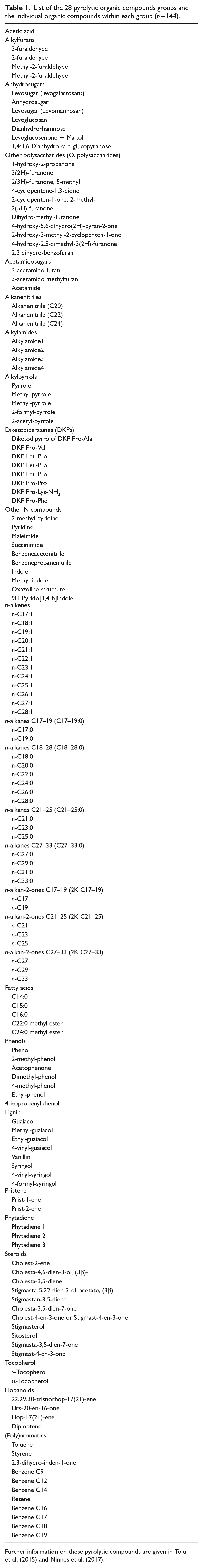
Further information on these pyrolytic compounds are given in Tolu et al. (2015) and Ninnes et al. (2017).

Statistical analyzes

A first step in our analyses was to confirm that undiluted DRIFT spectroscopy can be used to estimate the TOC content in lake sediments. For this initial proof-of-concept we first developed a general calibration model using DRIFT spectra of untreated samples and the corresponding TOC concentrations in the 93-lake northern Swedish training set (Bigler and Hall, 2002; Rosén et al., 2010). By building a model on samples from a large number of lakes it is possible to compare the performance of our model to similar, existing models but which are based on spectra from samples diluted with KBr. For external validation, we applied the general northern Swedish model to the Holocene sediment cores from Dragsjön and Lång-Älgsjön. To demonstrate that our approach also performs well for site-specific conditions the Dragsjön core was then used to develop a local calibration model that was externally validated using the Lång-Älgsjön core.

Both TOC calibrations models were developed with PLSR in SIMCA 16.0 (Umetrics, Umeå, Sweden) using linearly baseline-corrected (3800–3750 and 2200–2210 cm⁻¹, Opus Interface) DRIFT spectra (3750–400 cm⁻¹). For the general northern Swedish model all data were centered. For the local model data were centered and standardized to unit variance (z-scored). The internal predictive performance of the models, that is, how well the DRIFT spectra predicts TOC content for the training sets, was evaluated with the coefficient of determination from seven-fold cross-validation (R²_CV) and with the root mean squared error of cross-validation (RMSECV, in % TOC). The external predictive ability of the models, that is, how well the models predict TOC content when applied to samples not used in the model, but with known TOC contents, was evaluated with the coefficient of determination (R²) and the root mean squared error of prediction (RMSEP, in % TOC).

For analysis of the qualitative OM sediment composition in the cores from Dragsjön and Lång-Älgsjön the main spectral peaks within the range 3750–400 cm⁻¹ were identified with the andurinha R application (Álvarez Fernández and Martínez Cortizas, 2020). This application provides the average, standard deviation and second derivative spectra, with the latter used for extraction of the main spectral peaks from baseline corrected spectra (3800–3750 and 2200–2210 cm⁻¹) for each sediment record. The main DRIFT spectral signals within the reduced spectra were extracted with PCA on standardized absorbance data in the R package “Psych” with a varimax rotation applied to maximize the variable loadings on the components. Principal component analysis was also applied to the 28 pyrolytic compound groups to enable comparison between DRIFTS and pyrolytic OM composition. The comparison was done using bivariate correlation coefficients between respective component scores and passively plotting DRIFT spectra components in the pyrolytic PCA loading plots. All principal components retained for the spectral and pyrolytic PCAs have eigenvalues >1.

Results and discussion

Reference DRIFT spectra of untreated samples and samples diluted with KBr

DRIFT absorbance spectra for the untreated reference samples show good coherence with published spectra for similar types of samples but which have been diluted with KBr. Untreated spectra for decomposed Sphagnum peat (Figures 1a and S2) show characteristic bands for O–H stretching of phenolic and aliphatic groups (3600–3200 cm⁻¹); C–H stretching of aliphatics (2925–2850 cm⁻¹, Niemeyer et al., 1992); C=O stretching of esters, aldehydes, ketones and carboxylic acids (1750–1670 cm⁻¹, Marchessault, 1962), and C–O and O–H stretching of aliphatic alcohols and C–H deformation of aromatics (1155–1000 cm⁻¹, Orem et al., 1996; Pandey, 1999; Zaccheo et al., 2002). The only difference in the DRIFT spectra between the untreated and the diluted samples is the slightly lower intensity of the broad band at 1120–1000 cm⁻¹, but specular distortion effects are effectively absent. For bSi, the DRIFT spectra of untreated and diluted samples are near identical above 1500 cm⁻¹ and below this region characteristic bands linked to Si–OH stretching (947 cm⁻¹) and Si–O–Si stretching (~800 cm⁻¹, Farmer, 1974) are easily identified (Figures 1b and S5). The DRIFT spectra of the untreated sample deviate as expected in the 1400–1000 and 700–400 cm⁻¹ regions. Here, specular distortion in the form of band reversal (1270–1000 cm⁻¹ and 500–400 cm⁻¹) and Fresnel peaks (1350 and 530 cm⁻¹) mask the broad bands linked to Si–O stretching (1100 cm⁻¹) and Si–O bending (470 cm⁻¹), which are present in the DRIFT spectra of the sample diluted with KBr. The same distortion effects are present in the DRIFT spectra of untreated samples of the Na-rich montmorillonite clay, with band reversals at 1070, 530, and 470 cm⁻¹ and Fresnel peaks at 1270 and 650 cm⁻¹ (Figures 1c and S6). However, bands necessary for identification of silicate mineral phases remain intact, including bands linked to Si–O stretching (802/786 cm⁻¹ doublet) and bending (695 cm⁻¹) of quartz and feldspars (Farmer, 1974), and the strong band between 3700–3600 cm^-1 characteristic of structural O–H vibrations in clays (Madejova and Komadel, 2001). Absorbance and second derivative spectra, peak positions, peak assignments and references for peak assignments for all five reference samples are presented in figures S2–6.

Figure 1.

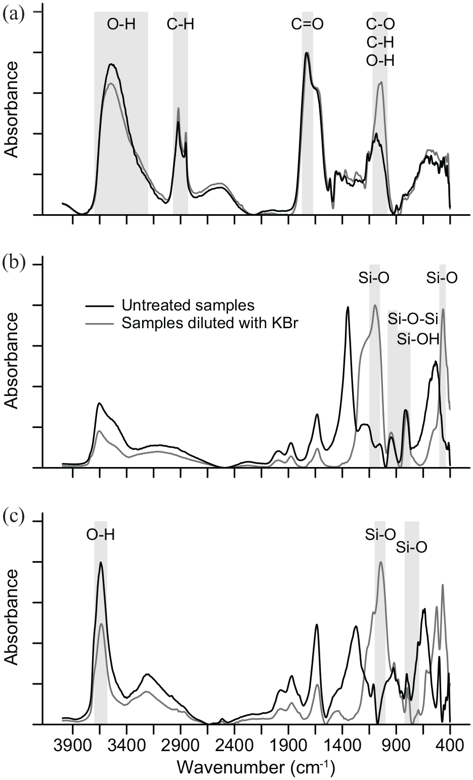
DRIFT absorbance spectra for reference samples (a) Sphagnum peat (CRM NJV 942), (b) biogenic silica, (c) Montmorillonite clay (SWy-2). Untreated samples are shown in black and samples diluted with KBr in gray. Data are baseline corrected (adaptive, coarseness 15, offset 0), smoothed (Savitsky–Golay, interval 10, polynomial order 3) and peak normalized (SpectraGryph v1.2.14; Menges 2016–2020) for visualization purposes. Vertical gray bars refer to absorbance bands mentioned in the text.

DRIFT spectra of untreated lake-sediment core samples

Absorbance spectra for Dragsjön (Figure 2) and Lång-Älgsjön (Figure S7) are very similar and characterized by high absorbance in four broad wavenumber regions. The first region, 3600–3000 cm⁻¹, corresponds to O–H, N–H and C=C stretching of organics, such as polysaccharides, phenols, alcohols and proteins (Shurvell, 2006), as well as to O–H stretching in bSi, silicate minerals and freely adsorbed water (Farmer, 1974). The second region, 2950–2850 cm⁻¹, corresponds to C–H stretching of aliphatics and aromatics (Boeriu et al., 2004; Niemeyer et al., 1992), and the third region, 1700–1000 cm⁻¹, to vibrations of a range of functional groups including carbonyl C=O vibrations in organic acids and proteins; C=C, C=N and N–H vibrations of aromatics and proteins; C–O–C and C–OH of alcohols, ethers and sugars, and C–H deformation of aliphatics (Shurvell, 2006). The fourth region, 750–400 cm⁻¹, corresponds to vibrations of polysaccharides, aliphatics, and minerals such as silicates and iron oxides (Farmer, 1974; Shurvell, 2006). Each of the two Holocene sequences includes two basal samples characterized by postglacial, silty clay with low (~ <5% TOC) organic contents. These samples have a peak at ~3620 cm⁻¹, linked to structural O–H vibrations in clay (Madejova and Komadel, 2001), Si–O overtone and combination bands at 2000–1800 cm⁻¹ (Nguyen et al., 1991), and characteristic Si–O bending and stretching peaks at 697, 772, 790, and 810 cm⁻¹ (Farmer, 1974). Standard deviation spectra calculated for all Dragsjön samples (n = 97) and with the basal samples removed (n = 95) clearly highlight these differences.

Figure 2.

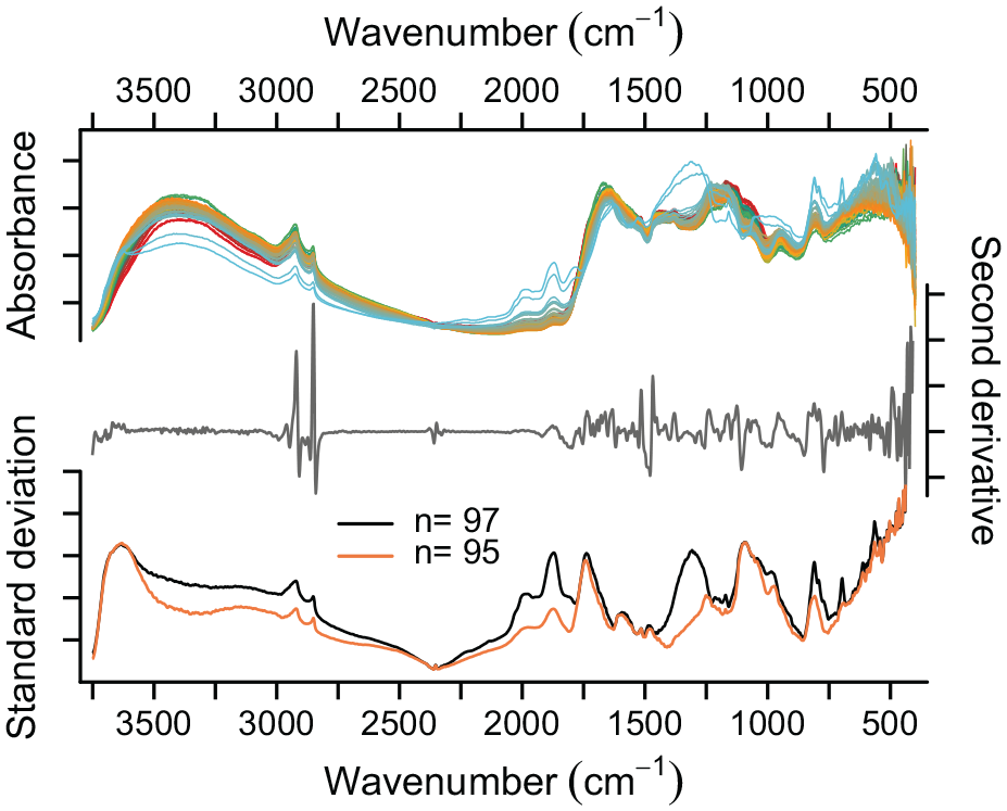
Relative absorbance, summed second derivative and standard deviation for lake sediment samples from Dragsjön. Standard deviation spectra are calculated for all samples (n = 97) and with the basal samples (two light blue lines in top panel) removed (n = 95).

Sediment TOC quantification with DRIFT spectra from untreated samples

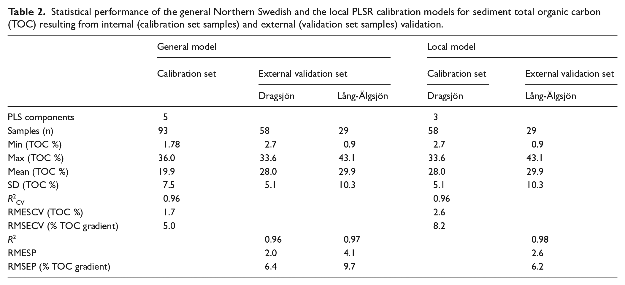
Our models for TOC quantification in lake sediments use the common DRIFTS technique coupled with PLSR, but contrast with previous work on lake sediments by using untreated samples for analysis. The general calibration for sediment TOC based on DRIFT spectra and TOC content for the northern Swedish training set (n = 93) resulted in a 5-component model with an R²_CV of 0.96 between the quantitative TOC measurements obtained with conventional elemental analysis and the PLSR-predicted TOC content, and a prediction error (RMSECV) of 1.7% (Table 2 and Figure 3). The first three latent components capture 89% of the variation in the spectral signal (DRIFT spectra, x-variables) and 94% in the TOC (y-variable). Loadings on components 1–3 expressed as weight vectors (w*c) show that wavenumbers 3600–2250, 1780–930, and 600–400 cm⁻¹ are strongly positively correlated to TOC.

Table 2.

Statistical performance of the general Northern Swedish and the local PLSR calibration models for sediment total organic carbon (TOC) resulting from internal (calibration set samples) and external (validation set samples) validation.

	General model			Local model
	Calibration set	External validation set		Calibration set	External validation set
	Calibration set	Dragsjön	Lång-Älgsjön	Dragsjön	Lång-Älgsjön
PLS components	5			3
Samples (n)	93	58	29	58	29
Min (TOC %)	1.78	2.7	0.9	2.7	0.9
Max (TOC %)	36.0	33.6	43.1	33.6	43.1
Mean (TOC %)	19.9	28.0	29.9	28.0	29.9
SD (TOC %)	7.5	5.1	10.3	5.1	10.3
R ² _CV	0.96			0.96
RMESCV (TOC %)	1.7			2.6
RMSECV (% TOC gradient)	5.0			8.2
R ²		0.96	0.97		0.98
RMESP		2.0	4.1		2.6
RMSEP (% TOC gradient)		6.4	9.7		6.2

Figure 3.

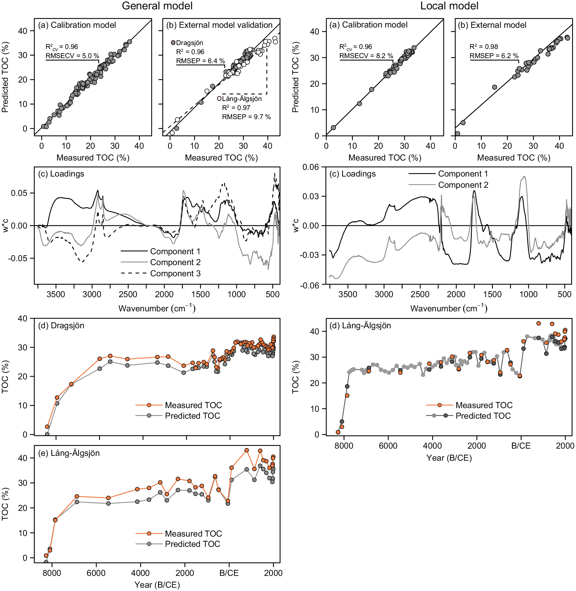
The general TOC calibration model (left) with measured sediment TOC concentrations versus DRIFTS predicted TOC concentrations for (a) the PLSR calibration model based on samples from the northern Swedish calibration training set (n = 93); (b) the external model validation using samples from Dragsjön (n = 58) and Lång-Älgsjön (n = 29); (c) loadings on the first three components of the calibration model, expressed as weight vectors (w*c), where positive weight vectors indicate wavenumbers positively correlated to the TOC concentration and negative weight vectors wavenumbers negatively correlated to TOC concentration, down-core trends for measured and predicted TOC concentrations for the external validation for (d) Dragsjön, and (e) Lång-Älgsjön. The local TOC calibration model (right) with measured sediment TOC concentrations versus DRIFTS predicted TOC concentrations for (a) the PLSR calibration model based samples from Dragsjön (n = 58); and (b) the external model validation using samples from Lång-Älgsjön (n = 29); c) loadings on the first three components of the calibration model, expressed as weight vectors (w*c), where positive weight vectors indicate wavenumbers positively correlated to the TOC concentration and negative weight vectors wavenumbers negatively correlated to TOC concentration, and (d) down-core trends for measured and predicted TOC concentrations for Lång-Älgsjön, where orange and dark gray circles represent the validation samples (n = 29) and light gray circles samples with model-predicted TOC only (n = 62).

The local calibration model based on DRIFT spectra and TOC content for Dragsjön (n = 58) resulted in a 3-component model with an R²_CV of 0.96 between the quantitative TOC measurements obtained with conventional elemental analysis and the PLSR-predicted TOC content, and a prediction error (RMSECV) of 2.6% (Table 2, Figure 3). The first two latent components capture 78% of the variation in the DRIFT spectra and 92% of the TOC. Loadings on components 1 and 2 show that wavenumbers 3500–3250, 3000–2235, 2214–2200, 1800–1640, and 1150–1026 cm⁻¹ are strongly positively correlated to TOC. Thus, for both models C–H stretching and overtones in aliphatics at 3000–2650 cm⁻¹; C=O stretching in carbonyl groups (1800–1640 cm⁻¹), and C–O and O–H stretching and deformation in polysaccharides, cellulose and lignin (1180–995 cm⁻¹) are important regions. The same three regions underpin calibration models for TOC and OM in soils and lake sediments based on samples diluted with KBr (Janik and Skjemstad, 1995; Rosén et al., 2010, 2011; Viscarra Rossel et al., 2006; Vogel et al., 2008), with the 3000–2800 cm⁻¹ region particularly important for the quantification of OM, TOC and humic substances in estuarine sediments (Alaoui et al., 2011; Tremblay and Gagné, 2002).

When the general northern Swedish model is applied to the sediment sequences from Dragsjön (R² = 0.96, RMSEP = 6.4% of gradient) and Lång-Älgsjön (R² = 0.97, RMSEP = 9.7% of gradient) the downcore trends are captured well, but concentrations are slightly underestimated for most samples (Figure 3). These underestimations likely occur because the samples in the northern Swedish training set to some extent are qualitatively different from the sediments in Dragsjön and Lång-Älgsjön, despite the comparable quantitative TOC ranges. These differences are captured by the contribution of each wavenumber to the PLSR models. While the same general regions are important for both models, there are notable differences particularly within the 3500–3000, 2215–2070, 1600–1200 cm⁻¹ regions (Figure 3). Accordingly, the local model based on samples from Dragsjön more accurately predicts sediment TOC concentrations in Lång-Älgsjön (R² = 0.98, RMSEP = 6.2), particularly for samples that fall within the range of concentrations that are well-represented in the calibration model (~23–34% TOC).

For both of our models, validation samples with measured TOC concentrations >34–36% are underestimated due to spectral saturation of these samples, which contributes to the higher RMSEP for Lång-Älgsjön than Dragsjön with the general northern Swedish model. The same issue was reported by Rosén et al. (2011) for samples diluted with KBr when TOC exceeded ~35%. When saturation occurs there is a deviation from the expected linear relationship between concentration and absorbance at the high end of concentrations, such that when the linear calibration model is applied to these samples, predicted TOC is underestimated. Here, dilution with alkali halides can be used to reduce band intensities and create models optimized for higher TOC ranges (Rosén et al., 2011). However, specular saturation will only be a problem for TOC analysis on untreated samples for lakes with highly organic sediment, such as those found in the upper part of the Lång-Älgsjön record, whereas most lake sediments will have TOC concentrations below 35%. For example, in the 93-lake northern Swedish training set only one lake exceeds 35% TOC, and in the 3164-lake training set spanning from polar desert to boreal forest environments used by Rosén et al. (2011), only ~1% of the lakes exceeded 35% TOC.

The performances of both models are nonetheless comparable to other calibration models that use DRIFT spectra, whether untreated estuarine sediment samples (Alaoui et al., 2011) or lake-sediment samples diluted with KBr (Vogel et al., 2008). The most comparable TOC ranges are those by Rosén et al. (2010, 2011), in which concentrations in lake sediment range from 0 to ~30–41% TOC, for a similar or higher number of samples (n = 94–3164, R²_CV = 0.83–0.98, RMESCV_gradient = 6.1–7.7%). Our results verify that lake-sediment TOC concentrations can be estimated using DRIFT spectra of untreated samples but that the accuracy of estimated values may differ between general and more lake-specific models. We expect that a more robust calibration model would result from a calibration data set that covers the entire qualitative sample range of the predictive data set, alternatively selecting a subset of samples for TOC analysis to develop a lake-specific calibration.

Qualitative sediment OM composition

Principal component analysis of lake sediment spectra

With help of the open-source andurinha R application, we identified 72 and 74 peaks from the second derivative of the DRIFT spectra for Dragsjön and Lång-Älgsjön. Preliminary PCAs on the absorbance spectra for these peaks enabled identification of wavenumbers associated with each of the three main lake sediment fractions (OM, mineral matter and bSi). Groups of wavenumbers identified as capturing mineral matter (i.e. all wavenumbers with negative or positive loadings on a particular component) were subsequently removed in a couple of successive PCAs such that the final PCAs included only organic and bSi components. Minerogenic wavenumbers were removed to make the comparison with the organic pyrolytic data more intuitive and because approaches for qualitative and quantitative analysis of mineral matter with MIR has been done elsewhere (e.g. Hahn et al., 2018; Kanbar et al., 2021; Martínez Cortizas et al., 2021a). Their removal does not affect the order of the organic components nor which components the wavenumbers load on, with the exception of one wavenumber for Dragsjön and four for Lång-Älgsjön. Wavenumbers associated with the bSi fraction were kept in the final PCAs because these bSi components appeared to also carry partial polysaccharide signals. Removing them does not alter the PCA results for Dragsjön, suggesting only a small polysaccharide signal, but weakens the polysaccharide signal for Lång-Älgsjön, suggesting a larger partial signal. For reference purposes the PCAs performed on the initial 72 and 74 for peaks are shown in Figure S8. The final PCAs on wavenumbers associated with OM and bSi include 43 spectral peaks for Dragsjön and 55 peaks for Lång-Älgsjön (Figure 4).

Figure 4.

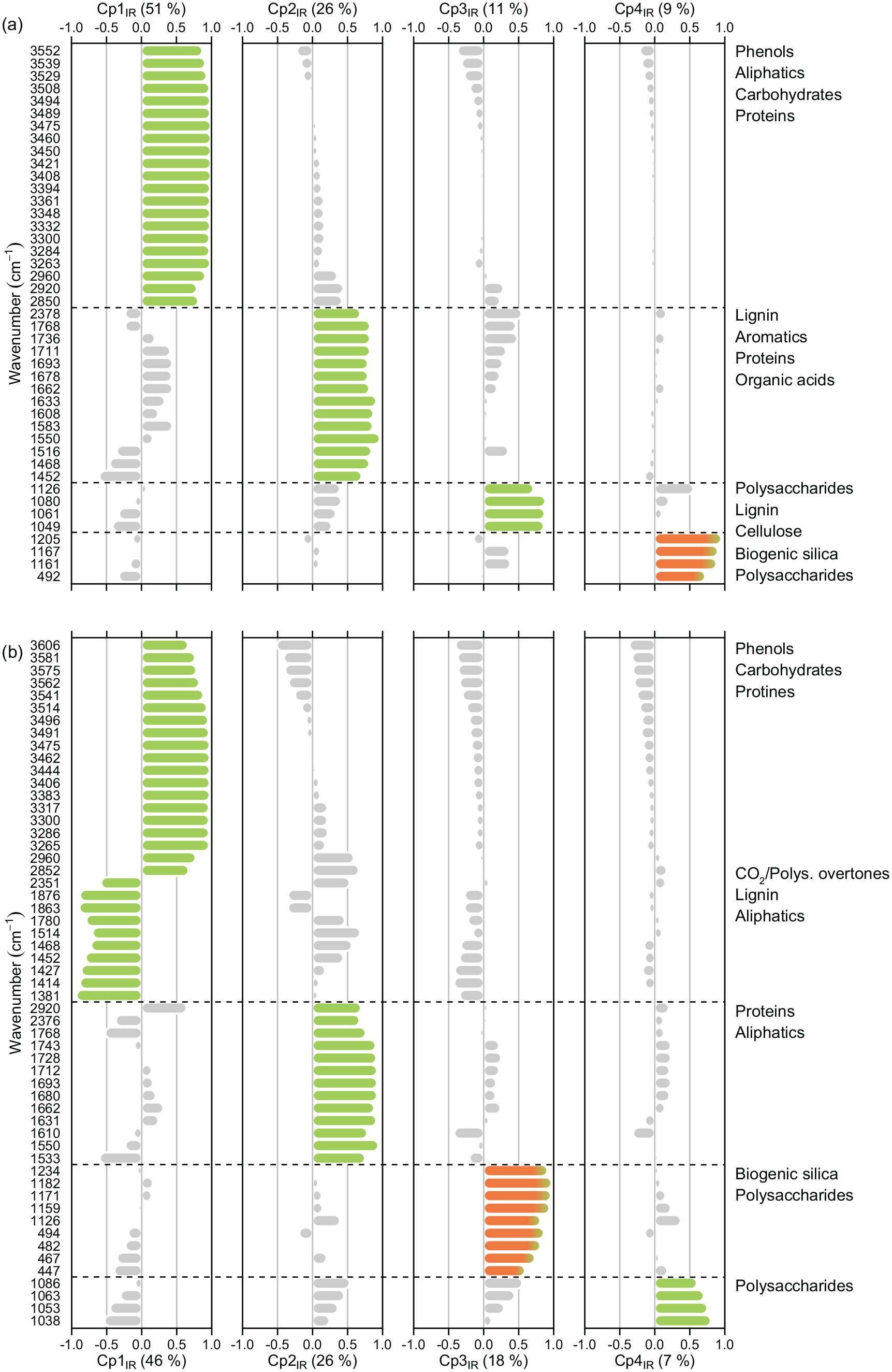
Principal component analyses of DRIFT spectra from untreated samples for (a) the 43 peaks capturing OM and bSi in Dragsjön, and (b) the absorbance spectra for the 55 peaks capturing OM and bSi in Lång-Älgsjön. Wavenumbers are ordered by component based on their strongest positive or negative loading, and colored by sediment fraction; organics (green), bSi (orange) and other variance allocation (light gray).

For Dragsjön the first four components of the final PCA capture 97% of the total spectral variance. The first component (Cp1_IR, 51% spectral variance, Figure 4a, Table S4) has positive loadings for wavenumbers associated with O–H and N–H vibrations of polysaccharides, phenols and proteins (3552–3263 cm⁻¹) and C–H stretching of aliphatics and aromatics (2960–2850 cm⁻¹). Component 2 (Cp2_IR, 26% spectral variance) has positive loadings for wavenumbers associated with CO₂ (an impurity) or possibly polysaccharide overtones (2378 cm⁻¹, Coates, 2000), C=O stretching in organic acids (1768–1693 cm⁻¹), C=O stretching, N–H bending and C=C stretching of proteins and aliphatics (1678–1633, 1583–1150, and 1452 cm⁻¹); as well as C=C stretching and C–H deformation of lignin and aromatics (1662, 1608, 1516, and 1468 cm⁻¹) (López Pasquali and Herrera, 1997; Marchessault, 1962; Sigee et al., 2002). The third component (Cp3_IR, 11% spectral variance) has positive loadings for wavenumbers 1126 and 1080–1049 cm⁻¹, most likely associated with C–O, C–H and O–H vibrations in lignin and intact polysaccharides (Kubo and Kadla, 2005; Mathlouthi and Koenig, 1986; Sigee et al., 2002). Component 4 (Cp4_IR, 9% spectral variance), has positive loadings for wavenumbers 1205, 1167, 1161 cm⁻¹ and 492 cm⁻¹ (Table S4). These five wavenumbers are likely to represent Si–O stretching and bending in bSi from diatomaceous algae because bSi has two main bands centered on 1100 and 470 cm⁻¹ (Gendron-Badou et al., 2003). It cannot, however, be excluded that at least part of this signal represents polysaccharides because the main band of C–O vibrations in polysaccharides overlaps with the main band in bSi, although typically centered lower, around 1050 cm⁻¹ (Sigee et al., 2002). A full list of vibrational modes, component loadings and communalities (% of variance explained for each component) for Dragsjön are given in Table S4.

For Lång-Älgsjön, the first four components capture 97% of the spectral variance. Component 1 (Cp1_IR, 46% spectral variance, Figure 4b, Table S5) has positive loadings associated with O–H and N–H vibrations (3606–3265 cm⁻¹), and C–H stretching (2690 and 2852 cm⁻¹). Wavenumbers with negative loadings are associated with vibrations of CO₂ or polysaccharide overtones (2351 cm⁻¹), C–H overtones and combination bands (1876 and 1863 cm⁻¹), C=O stretching in organic acids and C=C stretching and C–H deformation in lignin and aliphatics (1514–1381 cm⁻¹). The aliphatic wavenumber 2920 cm⁻¹ is found on component 2 (Cp2_IR, 26% spectral variance) together with CO₂/polysaccharide overtones (2376 cm⁻¹), C=O stretching in organic acids (1769–1693 cm⁻¹) and C=O and N–H vibrations in proteins (1680–1550 cm⁻¹). Component 3 (Cp3_IR, 18% spectral variance) has positive loadings for wavenumber regions 1234–1126 cm⁻¹ and 494–447 cm⁻¹. Similar to Cp4_IR for Dragsjön, this component likely primarily carries information associated with Si–O stretching and bending in bSi, because the main polysaccharide signal appears to be captured by the slightly lower wavenumbers (1086–1038 cm⁻¹, Mathlouthi and Koenig, 1986) on component 4 (Cp4_IR, 7% spectral variance), but may in part also carry a polysaccharide signal. A full list of vibrational modes, component loadings and communalities for Lång-Älgsjön are given in Table S5.

Comparison of spectral and pyrolytic OM composition

Dragsjön

Passive plotting of the four spectral components (Cp1–4_IR) in the pyrolytic components 1 and 2 (Cp1–2_PY) space supports the interpretation of Cp3_IR (1126–1049 cm⁻¹) as capturing primarily polysaccharides. This is because Cp3_IR plots with the indicators of intact OM in the bottom left quadrant (Figure 5a). These include anhydrosugars, which primarily are indicators of intact polysaccharides from plants (Pouwels et al., 1987), but also found in some algae (Piloni et al., 2021); 4-isopropenylphenol, a pyrolysis product of Sphagnum acid and sensitive to aerobic degradation (Schellekens et al., 2015); and the other polysaccharides from mixed origins (i.e. microbes, plants, algae; Nguyen et al., 2003; Pouwels et al., 1987).

Figure 5.

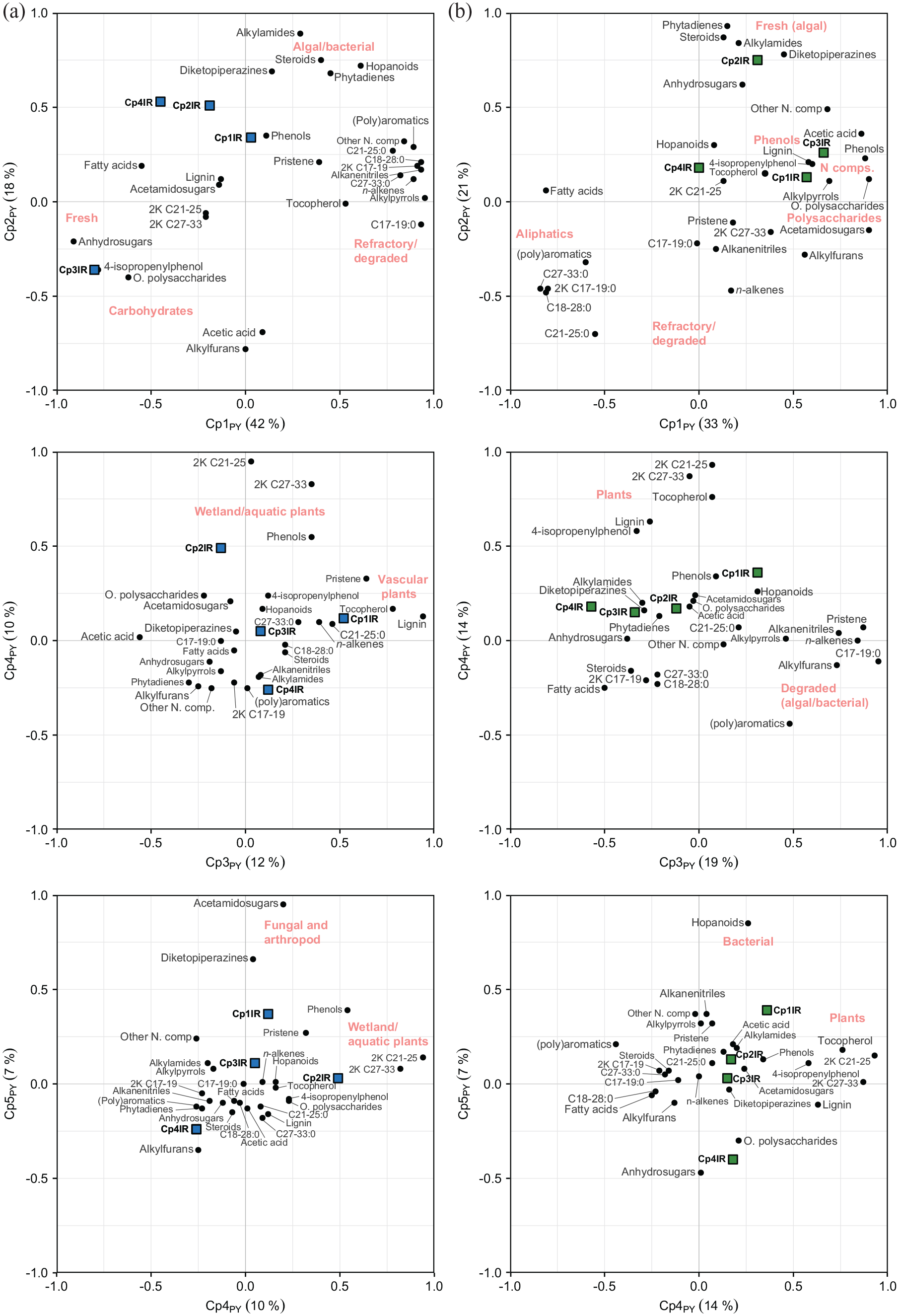
Loadings for pyrolytic principal components 1–4 (Cp1–4_PY) based the 28 pyrolytic organic compound groups for (a) Dragsjön and (b) Lång-Älgsjön. Filled circles correspond to pyrolytic compound groups and filled squares to the passively added spectral components Cp1–4_IR. C17–19:0, n-alkanes C17– 19; C18–28:0, n-alkanes C18–28; C21–25:0, n-alkanes C21–25; C27–33:0, n-alkanes C27–33; 2K C17–19, n-alkan-2-ones C17–19; 2K C21–25, n-alkan-2-ones C21–25; 2K C27–33, n-alkan-2-ones C27–33.

The second spectral component, Cp2_IR (2378, 1768–1452 cm⁻¹), plots in the upper left quadrant, half-way between the fatty acids on the negative side of Cp1_PY, here dominated by the relatively labile, short chain fatty acids (C14–16:0, Table 2) that are typical of aquatic OM (Cranwell et al., 1987; Han et al., 2022; Jaffé et al., 2001), and a group of pyrolysis products of algal and bacterial origins in the top right quadrant on the positive side of Cp2_PY. The latter includes hopanoids, which derive from bacterial membrane (Ourisson et al., 1987); the chlorophyll-derived phytadienes; the protein and amino acid-derived diketopiperazines (Fabbri et al., 2012); the mixed origin steroids (Volkman, 1986) and the alkylamides, which are dehydration products of algal macromolecules (Derenne et al., 1993) and possibly also secondary pyrolysis products of amino acids and proteins (Nierop and van Bergen, 2002). This combination of compound groups has previously been interpreted as algal-derived OM in a boreal lake sediment sequence from south-western Sweden (Tolu et al., 2017) and the location of Cp2_IR in the Cp1–2_PY space agrees with the partial protein and aliphatic spectral signal captured by Cp2_IR.

The fourth spectral component, Cp4_IR, interpreted as mainly a bSi signal with a minor polysaccharide signal (1205–1161 and 492 cm⁻¹), also plots in the upper left quadrant, partially capturing an algal and bacterial signal and partially a labile OM signal. This supports the bSi (i.e. algal) interpretation of Cp4_IR, but also the partial polysaccharide signal. The duality is also evident in down-core trends of Cp4_IR component scores and DRIFTS-based, PLSR-modeled bSi content (Figure 6a). The trends are coherent until ~1000 CE, but after this point, bSi content deviates from the increasing trend of Cp4_IR, probably due to the increase in polysaccharides content. Finally, Cp1_IR, capturing O–H vibrations of polysaccharides and phenols, C–H stretching of aliphatics, and N–H stretching in proteins (3552–2850 cm⁻¹), plots in the upper center of the plot, close to the pyrolytic compound group phenols.

Figure 6.

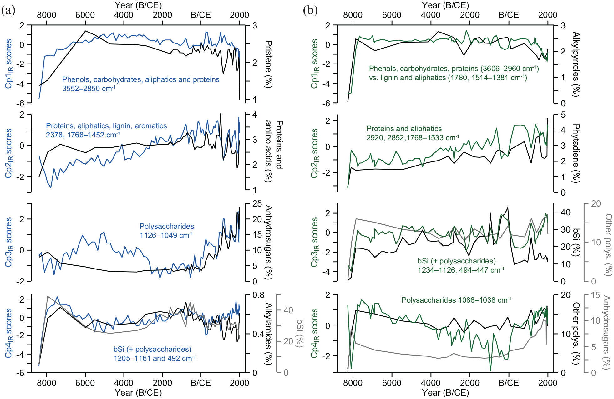
Down-core trends for spectral components Cp1_IR to Cp4_IR (blue and green lines), selected pyrolytic compound groups and sediment bSi content for the past ~8500 years in (a) Dragsjön and (b) Lång-Älgsjön. bSi (%) data for Lång-Älgsjön are from Meyer-Jacob et al. (2015).

In the pyrolytic components 3 and 4 (Cp3–4_PY) space, Cp1_IR (3552–2850 cm⁻¹) plots on the positive side of Cp3_PY where lignin, tocopherol, pristene, n-alkanes C21–25 and n-alkenes are found. Lignin include pyrolysis products of syringyl and guaiacyl methoxy-phenols and only derive from vascular plants (Saiz-Jimenez and De Leeuw, 1986). Tocopherols are lipophilic antioxidants produced exclusively by photosynthetic plants, algae and some cyanobacteria (DellaPenna and Pogson, 2006), and pristene pyrolytic or degradation products of tocopherol, and to a lesser extent chlorophyll (Goossens et al., 1984; Höld et al., 2001; Nguyen et al., 2003). The aliphatic n-alkanes C21–25 are found in both Sphagnum moss and in vascular plants (Bush and McInerney, 2013), but do also, along with the aliphatic n-alkenes, form during pyrolysis (Van Smeerdijk and Boon, 1987). These compounds indicate that Cp1_IR captures information on aliphatics and phenolic compounds, as well as proteins, of vascular plant origin.

The spectral component Cp2_IR (1768–1452 cm⁻¹) plots half way between the wetland indicators n-alkan-2-ones C21–25 and C27–33, and phenols on the positive side of Cp4_PY and the compound groups other polysaccharides and acetamidosugars on the negative side of Cp3_PY. The aliphatic n-alkan-2-ones C21–25 and C27–33 are ubiquitous in lake and wetland environments as components of various aquatic and peat-forming plants (Nichols and Huang, 2007; Ortiz et al., 2011; Qu et al., 1999) and the phenols derive from lignin (Faix et al., 1991; Saiz-Jimenez and De Leeuw, 1986), cellulose (Pouwels et al., 1989), non-lignin plant phenols (Schellekens et al., 2009) and proteins (van Heemst et al., 1999). This location of Cp2_IR strongly supports the mixed aliphatic, protein, lignin and aromatic signal captured by Cp2_IR.

Plotting of Cp1–4_IR in the pyrolytic components 4 and 5 (Cp4–5_PY) space shows that Cp1_IR plots in the upper center of the plot, the positive side of Cp5_PY. This component is driven by the chitin-derived acetamidosugars (Stankiewicz et al., 1996) and the protein and amino acid-derived diketopiperazines. In the plot space, however, Cp1_IR is located closer to the phenols and pristene, which further supports that Cp1_IR captures phenolic compounds, in addition to vascular plant-associated aliphatic and chlorophyll derivatives.

Lång-Älgsjön

Passive plotting of the four spectral components (Cp1–4_IR) in the pyrolytic components 1 and 2 (Cp1–2_PY) space shows that Cp1_IR, capturing the relative proportions of phenols, polysaccharides and proteins at 3606–2960 cm⁻¹ versus lignin and aliphatics at 1780 and 1514–1381 cm⁻¹ plots on the positive side of Cp1_PY together with a range of polysaccharide, phenol and protein-derived compounds groups (Figure 5b). Cp3_IR, capturing mainly a bSi signal (1234–1126 and 494–447 cm⁻¹), also plots with the pyrolytic compound groups to the right on Cp1_PY. The opposite side of Cp1_PY captures the fatty acids, (poly)aromatics and many of the aliphatic groups, which have in common very high relative abundances in the two silt and clay-rich basal samples. They likely represent refractory, or potentially shielded (Han et al., 2022), OM from the time of lake formation. The second spectral component, Cp2_IR, capturing aliphatics and proteins (2920–2852 and 1768–1533 cm⁻¹), plots with phytadiene, steroids, alkylamides and diketopiperazines, indicative of algal OM, on the positive side of Cp2_PY. Anhydrosugars also plot near these compound groups, as an indicator of intact OM, though a minor algal signal cannot be excluded. Cp2_IR plots closer to the algal OM compound groups for Lång-Älgsjön than for Dragsjön, probably because this spectral component includes predominantly vibrations of aliphatics and proteins, as opposed to also capturing vibrations of lignin and aromatics for Dragsjön.

In the pyrolytic components 3 and 4 (Cp3–4_PY) space, only Cp1_IR (3606–2960 cm⁻¹ vs 1780, 1514–1381 cm⁻¹) plots on the positive side of Cp3_PY, while the remaining three components plot on the negative side. The pyrolytic compound groups located on the positive side of Cp3_PY likely represent degraded algal and bacterial OM. These groups include the n-alkanes C17–19, representing direct inputs from aquatic plants and bacteria (López-Días et al., 2013; Qu et al., 1999), but also microbial oxidation of n-alkanes and decarboxylation of fatty acids (Ambles et al., 1993; Püttmann and Bracke, 1995); pristene, which are pyrolytic or degradation products of primarily tocopherol; alkanenitrile, derived from pyrolysis of algal macromolecules; the small alkylfurans, which may be derived from plant polysaccharides (Marbot, 1997; Pouwels et al., 1987) and bacterial sugars (Buurman et al., 2005); and the protein-derived alkylpyrroles (Nguyen et al., 2003). Compounds found on the negative side of Cp3_PY are instead the less-degraded compounds such as fatty acids, anhydrosugars, steroids and 4-isopropenylphenol. Along this gradient, Cp1_IR is located near the hopanoids and phenols, suggesting it carries a partial bacterial, more so than algal, signal, while the polysaccharide component, Cp4_IR (1086–1038 cm⁻¹), is located furthest left, near a cluster of compounds encompassing both intact polysaccharides (anhydrosugars) and algal OM indicators (alkylamides, diketopiperazines and phytadiene). Unlike for Dragsjön, none of the spectral components plot near the plant OM indicators, including n-alkan-2-ones C21–25 and C27–33, tocopherol, lignin and 4-isopropenylphenol, on Cp4_PY.

In the pyrolytic components 4 and 5 (Cp4–5_PY) space, the bacterial OM indicator hopanoids is located toward the top of the plot on the positive side of Cp5_PY, and pyrolysis products of intact polysaccharides are located toward the bottom, on the negative side. The spectral components are again found along a gradient, with Cp1_IR located the positive side of Cp5_PY, half-way between the hopanoids and the plant OM on Cp4_PY, and Cp4_IR down the bottom close to the other polysaccharides and the anhydrosugars. These patterns further support that Cp1_IR (3606–2960 cm⁻¹) represents a degraded OM fraction with a strong phenolic and proteinaceous signal, and the polysaccharides on Cp4_IR (1086–1038 cm⁻¹) the most-intact OM fraction in Lång-Älgsjön.

Temporal trends

The OM composition in these two lake-sediment cores was previously divided into three major phases based on the pyrolytic organic compounds (Ninnes et al., 2017). To further validate our DRIFTS approach as a stand-alone method to characterize OM composition a brief comparison of temporal changes may be highly informative. The earliest of the three phases identified by Ninnes et al. (2017) is the post-glacial phase (>7900 BCE), which represents the time of lake formation. Mineral matter initially dominates the sediment but as the catchments become vegetated and soils stabilize (Myrstener et al., 2021), the relative abundances of most pyrolytic organic compound groups increase rapidly (Figure 6). This phase is equally apparent in the spectral data, with initially low scores for all organic components, corroborating the relatively low, but increasing OM content. The second phase spans most of the Holocene, until ~300 CE, and is characterized by stable or slowly changing relative abundances of pyrolytic organic compounds. This phase represents a climatically warm, but linearly cooling, phase of the Holocene (Seppä et al., 2009), where most trends for both pyrolytic organic compound groups and spectral components either show unchanging (Lång-Älgsjön Cp1_IR, and Cp3_IR), or slowly increasing (Cp2_IR both lakes) or decreasing trends (Lång-Älgsjön Cp4_IR). Slow, millennial-scale fluctuations are seen in seen in Cp1_IR, Cp3_IR and Cp4_IR in Dragsjön. Minor fluctuations in the pyrolytic data during this phase are masked due to the lower sampling resolution in these sections of the cores, but the higher resolution spectral data corroborate that no rapid changes in OM composition occurred, with the exception for Cp3_IR (polysaccharides) in Dragsjön.

The third phase, spanning ~300 CE to present, is the most dynamic, hence also divided into three sub-phases. The first two are characterized by large increases in labile pyrolytic compound groups such as proteins and amino acids, anhydrosugars and 4-isopropenylphenol, but also in the aliphatic n-alkan-2-ones. These changes are probably linked to altered catchment inputs due to expansion of adjacent peatlands and/or the development of the floating, shoreline peat mats (Myrstener et al., 2021; Ninnes et al., 2017). Increased supply of OM from peat or Sphagnum, in combination with more rapid burial, would increase the proportion of polysaccharides in the sediment and also promote preservation of labile compounds (Ninnes et al., 2017). Spectral components that carry protein and polysaccharide signals similarly indicate large changes in OM composition during the first two sub-phases in both lakes.

During the third sub-phase, from 1970 CE to present, diagenetic processes are an important feature in the pyrolytic OM composition and possible to identify due to the high compositional detail provided by this technique, which allows for tracking of individual compounds (Ninnes et al., 2017). Diagenetic signals cannot be identified in the spectral components, nor in the spectra of individual wavenumbers of labile compounds or in ratios between labile and resistant compounds. This is possibly because the main wavenumbers for labile compounds, that is, polysaccharides, are not “clean,” but also carry other types of information, mainly on Si–O vibrations.

Summary – Application of undiluted MIR spectroscopy for analysis of lake-sediment OM composition

Our spectral analyses of two lake-sediment sequences highlight the advantages and potential of MIR, whether DRIFTS as used in here or ATR, using untreated samples to extract quantitative and qualitative data on lake-sediment OM composition. Here we outline a strategy for applying DRIFTS to analyze lake-sediment cores simply using dried and ground samples, allowing for high sampling resolution and much greater detailing of OM composition than other rapid and low-cost methods (e.g. C and N elemental analyzes along with their isotopes).

First, as expected, we show that sediment TOC concentrations can be modeled either with a general calibration model using a wide variety of sediment samples or with a local model developed from a subset of samples from the sediment record(s) of interest. These TOC models based on the DRIFT spectra of untreated samples have the same predictive abilities as models based on samples diluted with KBr and can be applied as a first step to provide estimates and to identify subsets of samples to be analyzed for C content in order to develop a more precise local model. Furthermore, our DRIFT spectra and measured C concentrations could potentially be used as a foundation for developing calibration models by anyone using similar DRIFTS instrumentation. Previous work on DRIFT spectra from untreated soil, estuarine sediment and water samples show good results not only for C, but also for quantification of total N and other major components, including humic substances and specific compounds groups such as amino acids and amino sugars (e.g. Alaoui et al., 2011; Matamala et al., 2019; Reeves et al., 2001; Tremblay et al., 2011). Hence, there is great potential for development of quantitative calibrations based DRIFT spectra of untreated samples for broad scale characterization of lake sediments.

Second, and more importantly for our aim, using the open-source processing pipeline with peak selection and reduction based on second derivative spectra developed by Álvarez Fernández and Martínez Cortizas (2020) in combination with PCA, the DRIFT spectra can be used to establish qualitative compositional changes in OM, as well as the minerogenic and to a large extent biogenic sediment fractions. Within the organic fraction, compound groups such as aromatics, lignin, aliphatics, proteins and polysaccharides could readily be identified in our two Holocene sediment records. As such, MIR can be used as a rapid stand-alone method for OM characterization or function as a screening process for more-specific, time-intensive analyses, such as Py-GC/MS or GC/MS and LC/MS methods requiring sample extraction, but which can further tease apart the OM composition, and identify sources and degradation status. A next step can be to develop predictive models based on MIR and pyrolytic data for modeling of greater sample compound diversity to reveal more about temporal OM changes.

Supplemental Material

sj-pdf-4-hol-10.1177_09596836231211872 – Supplemental material for Application of mid-infrared spectroscopy for the quantitative and qualitative analysis of organic matter in Holocene sediment records

Supplemental material, sj-pdf-4-hol-10.1177_09596836231211872 for Application of mid-infrared spectroscopy for the quantitative and qualitative analysis of organic matter in Holocene sediment records by Sofia Ninnes, Carsten Meyer-Jacob, Julie Tolu, Richard Bindler and Antonio Martínez Cortizas in The Holocene

Research Data

sj-xlsx-1-hol-10.1177_09596836231211872 – Research Data for Application of mid-infrared spectroscopy for the quantitative and qualitative analysis of organic matter in Holocene sediment records

Research Data, sj-xlsx-1-hol-10.1177_09596836231211872 for Application of mid-infrared spectroscopy for the quantitative and qualitative analysis of organic matter in Holocene sediment records by Sofia Ninnes, Carsten Meyer-Jacob, Julie Tolu, Richard Bindler and Antonio Martínez Cortizas in The Holocene

This article is distributed under the terms of the Creative Commons Attribution 4.0 License (http://www.creativecommons.org/licenses/by/4.0/) which permits any use, reproduction and distribution of the work without further permission provided the original work is attributed as specified on the SAGE and Open Access pages (https://us.sagepub.com/en-us/nam/open-access-at-sage).

Research Data

sj-xlsx-2-hol-10.1177_09596836231211872 – Research Data for Application of mid-infrared spectroscopy for the quantitative and qualitative analysis of organic matter in Holocene sediment records

Research Data, sj-xlsx-2-hol-10.1177_09596836231211872 for Application of mid-infrared spectroscopy for the quantitative and qualitative analysis of organic matter in Holocene sediment records by Sofia Ninnes, Carsten Meyer-Jacob, Julie Tolu, Richard Bindler and Antonio Martínez Cortizas in The Holocene

Research Data

sj-xlsx-3-hol-10.1177_09596836231211872 – Research Data for Application of mid-infrared spectroscopy for the quantitative and qualitative analysis of organic matter in Holocene sediment records

Research Data, sj-xlsx-3-hol-10.1177_09596836231211872 for Application of mid-infrared spectroscopy for the quantitative and qualitative analysis of organic matter in Holocene sediment records by Sofia Ninnes, Carsten Meyer-Jacob, Julie Tolu, Richard Bindler and Antonio Martínez Cortizas in The Holocene

Footnotes

Acknowledgements

We acknowledge and thank Martin Plöhn and Christiane Funk for supplying the algal reference sample and Umeå Plant Science Center for making the Py-GC/MS available to us. We also thank Alexander Francke and one anonymous reviewer for providing valuable comments that improved the manuscript.

Data availability

Spectroscopic data sets, including total organic carbon content, are available on the Figshare repository platform. Other supporting information can be found in the supplementary materials.

Funding

The author(s) disclosed receipt of the following financial support for the research, authorship, and/or publication of this article: This research was supported by Knut och Alice Wallenbergs Stiftelse [grant number 2016.0083] and the Swedish Research Council [grant number 2014-05219].

ORCID iDs

Sofia Ninnes

Carsten Meyer-Jacob

Antonio Martínez Cortizas

Supplemental material

Supplemental material for this article is available online.

References

Alaoui

Léger

Gagné

, et al. (2011) Assessment of estuarine sediment and sedimentary organic matter properties by infrared reflectance spectroscopy. Chemical Geology: Isotope Geoscience section 286: 290–300.

Álvarez Fernández

Martínez Cortizas

(2020) andurinha: Make spectroscopic data processing easier. R package version 0.0.2. Available at: https://CRAN.R-project.org/package=andurinha

Ambles

Jambu

Jacquesy

J-C

, et al. (1993) Changes in the ketone portion of lipidic components during the decomposition of plant debris in A hydromorphic forest-Podzol. Soil Science 156: 49–56.

Aryee

ANA

van de Voort

Simpson

(2009) FTIR determination of free fatty acids in fish oils intended for biodiesel production. Process Biochemistry 44: 401–405.

Bigler

Hall

(2002) Diatoms as indicators of climatic and limnological change in Swedish lapland: A 100-lake calibration set and its validation for paleoecological reconstructions. Journal of Paleolimnology 27: 97–115.

Boeriu

Bravo

Gosselink

RJA

, et al. (2004) Characterisation of structure-dependent functional properties of lignin with infrared spectroscopy. Industrial Crops and Products 20: 205–218.

Brisset

Miramont

Guiter

, et al. (2013) Non-reversible geosystem destabilisation at 4200 cal. BP: Sedimentological, geochemical and botanical markers of soil erosion recorded in a Mediterranean alpine lake. The Holocene 23: 1863–1874.

Bush

McInerney

(2013) Leaf wax n-alkane distributions in and across modern plants: Implications for paleoecology and chemotaxonomy. Geochimica et Cosmochimica Acta 117: 161–179.

Buurman

Van Bergen

Jongmans

, et al. (2005) Spatial and temporal variation in podzol organic matter studied by pyrolysis-gas chromatography/mass spectrometry and micromorphology. European Journal of Soil Science 56: 253–270.

10.

Cadd

Tyler

Tibby

, et al. (2020) The potential for rapid determination of charcoal from wetland sediments using infrared spectroscopy. Palaeogeography, Palaeoclimatology, Palaeoecology 542: 109562.

11.

Coates

(2000) Interpretation of infrared spectra, a practical approach. In: Meyers

(ed.) Encyclopedia of Analytical Chemistry. Chichester: JohnWiley & Sons Ltd, pp. 10815–10837.

12.

Cranwell

Eglinton

Robinson

(1987) Lipids of aquatic organisms as potential contributors to lacustrine sediments-ii. Organic Geochemistry 11: 513–527.

13.

DellaPenna

Pogson

(2006) Vitamin synthesis in plants: tocopherols and carotenoids. Annual Review of Plant Biology 57: 711–738.

14.

Derenne

Largeau

Taulelle

(1993) Occurrence of non-hydrolysable amides in the macromolecular constituent of Scenedesmus quadricauda cell wall as revealed by 15N NMR: Origin of n-alkylnitriles in pyrolysates of ultralaminae-containing kerogens. Geochimica et Cosmochimica Acta 57: 851–857.

15.

Fabbri

Adamiano

Falini

, et al. (2012) Analytical pyrolysis of dipeptides containing proline and amino acids with polar side chains. Novel 2,5-diketopiperazine markers in the pyrolysates of proteins. Journal of Analytical and Applied Pyrolysis 95: 145–155.

16.

Faix

Fortmann

Bremer

, et al. (1991) Thermal degradation products of wood: Gas chromatographic separation and mass spectrometric characterization. Holz als Roh- und Werkstoff 49: 213–219.

17.

Farmer

(1974) The layer silicates. In: Farmer

(ed.) The Infrared Spectra of Minerals. London: Mineralogical Society, pp.331–379.

18.

Gendron-Badou

Coradin

Maquet

, et al. (2003) Spectroscopic characterization of biogenic silica. Journal of Non-Crystalline Solids 316: 331–337.

19.

Goossens

de Leeuw

Schenck

, et al. (1984) Tocopherols as likely precursors of pristane in ancient sediments and crude oils. Nature 312: 440–442.

20.

Hahn

Kliem

Ohlendorf

, et al. (2013) Climate induced changes as registered in inorganic and organic sediment components from Laguna Potrok Aike (Argentina) during the past 51 ka. Quaternary Science Reviews 71: 154–166.

21.

Hahn

Vogel

Andó

, et al. (2018) Using Fourier transform infrared spectroscopy to determine mineral phases in sediments. Sedimentary Geology 375: 27–35.

22.

Han

Tolu

Deng

, et al. (2022) Long-term preservation of biomolecules in lake sediments: Potential importance of physical shielding by recalcitrant cell walls. PNAS Nexus 1: ac076.

23.

Hofko

Alavi

Grothe

, et al. (2017) Repeatability and sensitivity of FTIR ATR spectral analysis methods for bituminous binders. Materials and Structures 50: 187.

24.

Hofko

Porot

Falchetto Cannone

, et al. (2018) FTIR spectral analysis of bituminous binders: Reproducibility and impact of ageing temperature. Materials and Structures 51: 45.

25.

Höld

Schouten

Van der Gaast

, et al. (2001) Origin of prist-1-ene and prist-2-ene in kerogen pyrolysates. Chemical Geology: Isotope Geoscience section 172: 201–212.

26.

Holtvoeth

Vogel

Wagner

, et al. (2010) Lipid biomarkers in Holocene and glacial sediments from ancient Lake Ohrid (Macedonia, Albania). Biogeosciences 7: 3473–3489.

27.

Finney

Brubaker

(2001) Effects of Holocene Alnus expansion on aquatic productivity, nitrogen cycling, and soil development in southwestern Alaska. Ecosystems 4: 358–368.

28.

Jaffé

Mead

Hernandez

, et al. (2001) Origin and transport of sedimentary organic matter in two subtropical estuaries: A comparative, biomarker-based study. Organic Geochemistry 32: 507–526.

29.

Janik

Skjemstad

(1995) Characterization and analysis of soils using mid-infrared partial least-squares .2. Correlations with some laboratory data. Australian Journal of Soil Research 33: 637–650.

30.

Kanbar

Tran Le

Olajos

, et al. (2021) Tracking mineral and geochemical characteristics of Holocene lake sediments: The case of Hotagen, west-central Sweden. Journal of Soils and Sediments 21: 3150–3168.

31.

Kubo

Kadla

(2005) Hydrogen bonding in lignin: A fourier transform infrared model compound study. Biomacromolecules 6: 2815–2821.

32.

Kylander

Ampel

Wohlfarth

, et al. (2011) High-resolution X-ray fluorescence core scanning analysis of Les Echets (France) sedimentary sequence: New insights from chemical proxies. Journal of Quaternary Science 26: 109–117.

33.

López-Días

Blanco

Bechtel

, et al. (2013) Different source of n-alkanes and n-alkan-2-ones in a 6000cal. yr BP Sphagnum-rich temperate peat bog (Roñanzas, N Spain). Organic Geochemistry 57: 7–10.

34.

López Pasquali

Herrera

(1997) Pyrolysis of lignin and IR analysis of residues. Thermochimica Acta 293: 39–46.

35.

Madejova

Komadel

(2001) Baseline studies of the clay minerals society source clays: Introduction. Clays and Clay Minerals 49: 372–373.

36.

Marbot

(1997) The selection of pyrolysis temperatures for the analysis of humic substances and related materials 1. Cellulose and chitin. Journal of Analytical and Applied Pyrolysis 39: 97–104.

37.

Marchessault

(1962) Application of infra-red spectroscopy to cellulose and wood polysaccharides. Pure and Applied Chemistry. Chimie Pure et Appliquee 5: 107–130.

38.

Martínez Cortizas

López-Merino

Silva-Sánchez

, et al. (2021a) Investigating the mineral composition of peat by combining FTIR-ATR and multivariate analysis. Minerals 11: 1084.

39.

Martínez Cortizas

Sjöström

Ryberg

, et al. (2021b) 9000 years of changes in peat organic matter composition in store Mosse (Sweden) traced using FTIR-ATR. Boreas 50: 1161–1178.

40.

Matamala

Jastrow

Calderón

, et al. (2019) Predicting the decomposability of arctic tundra soil organic matter with mid infrared spectroscopy. Soil Biology and Biochemistry 129: 1–12.

41.

Mathlouthi

Koenig

(1986) Vibrational spectra of carbohydrates. Advances in Carbohydrate Chemistry and Biochemistry 44: 7–89.

42.

Maxson

Tibby

Marshall

, et al. (2021) Fourier transform infrared spectroscopy as a tracer of organic matter sources in lake sediments. Palaeogeography, Palaeoclimatology, Palaeoecology 581: 110622.

43.

Meyer-Jacob

Tolu

Bigler

, et al. (2015) Early land use and centennial scale changes in lake-water organic carbon prior to contemporary monitoring. Proceedings of the National Academy of Sciences of the United States of America 112: 6579–6584.

44.

Meyer-Jacob

Vogel

Gebhardt

, et al. (2014) Biogeochemical variability during the past 3.6 million years recorded by FTIR spectroscopy in the sediment record of Lake El’gygytgyn, Far East Russian Arctic. Climate of the Past 10: 209–220.

45.

Mirwald

Nura

Hofko

(2022) Recommendations for handling bitumen prior to FTIR spectroscopy. Materials and Structures 55: 1–17.

46.

Myrstener

Ninnes

Meyer-Jacob

, et al. (2021) Long-term development and trajectories of inferred lake-water organic carbon and pH in naturally acidic boreal lakes. Limnology and Oceanography 66: 2408–2422.

47.

Nguyen

Harvey

Zang

, et al. (2003) Preservation of algaenan and proteinaceous material during the oxic decay of Botryococcus braunii as revealed by pyrolysis-gas chromatography/mass spectrometry and ¹³ C NMR spectroscopy. Organic Geochemistry 34: 483–497.

48.

Nguyen

Janik

Raupach

(1991) Diffuse reflectance infrared fourier transform (DRIFT) spectroscopy in soil studies. Australian Journal of Soil Research 29: 49–67.

49.

Nichols

Huang

(2007) C23–C31 n-alkan-2-ones are biomarkers for the genus Sphagnum in freshwater peatlands. Organic Geochemistry 38: 1972–1976.

50.

Niemeyer

Chen

Bollag

J-

(1992) Characterization of humic acids, composts, and peat by diffuse reflectance Fourier-transform infrared spectroscopy. Soil Science Society of America Journal Soil Science Society of America 56: 135–140.

51.

Nierop

KGJ

van Bergen

(2002) Clay and ammonium catalyzed reactions of alkanols, alkanoic acids and esters under flash pyrolytic conditions. Journal of Analytical and Applied Pyrolysis 63: 197–208.

52.

Ninnes

Tolu

Meyer-Jacob

, et al. (2017) Investigating molecular changes in organic matter composition in two Holocene lake-sediment records from central Sweden using pyrolysis-gc/MS/MS. Journal of Geophysical Research Biogeosciences 122: 1423–1438.

53.

Orem

Burnett

Landing

, et al. (1991) Jellyfish Lake, Palau: Early diagenesis of organic matter in sediments of an anoxic marine lake. Limnology and Oceanography 36: 526–543.

54.

Orem

Neuzil

Lerch

, et al. (1996) Experimental early-stage coalification of a peat sample and a peatified wood sample from Indonesia. Organic Geochemistry 24: 111–125.

55.

Ortiz

Díaz-Bautista

Aldasoro

, et al. (2011) N-Alkan-2-ones in peat-forming plants from the Roñanzas ombrotrophic bog (Asturias, northern Spain). Organic Geochemistry 42: 586–592.

56.

Ourisson

Rohmer

Poralla

(1987) Prokaryotic hopanoids and other polyterpenoid sterol surrogates. Annual Review of Microbiology 41: 301–333.

57.

Pandey

(1999) A study of chemical structure of soft and hardwood and wood polymers by FTIR spectroscopy. Journal of Applied Polymer Science 71: 1969–1975.

58.

Pérez-Rodríguez

Gilfedder

Hermanns

, et al. (2016) Solar output controls periodicity in lake productivity and wetness at southernmost South America. Scientific Reports 6: 37521.

59.

Piloni

Daga

Urcelay

, et al. (2021) Experimental investigation on fast pyrolysis of freshwater algae. Prospects for alternative bio-fuel production. Algal Research 54: 102206.

60.

Pouwels

Eijkel

Boon

(1989) Curie-point pyrolysis-capillary gas chromatography-high-resolution mass spectrometry of microcrystalline cellulose. Journal of Analytical and Applied Pyrolysis 14: 237–280.

61.

Pouwels

Tom

Eijkel

, et al. (1987) Characterisation of Beech wood and its holocellulose and xylan fractions by pyrolysis-gas chromatography-mass spectrometry. Journal of Analytical and Applied Pyrolysis 11: 417–436.

62.

Püttmann

Bracke

(1995) Extractable organic compounds in the clay mineral sealing of a waste disposal site. International Journal of Rock Mechanics and Mining Sciences & Geomechanics 32: A375–A376.

63.

Dickman

Wang

, et al. (1999) Evidence for an aquatic plant origin of ketones found in Taihu lake sediments. Hydrobiologia 397: 149–154.

64.

Reeves

McCarty

Reeves

(2001) Mid-infrared diffuse reflectance spectroscopy for the quantitative analysis of agricultural soils. Journal of Agricultural and Food Chemistry 49: 766–772.

65.

Rosén

Vogel

Cunningham

, et al. (2010) Fourier transform infrared spectroscopy, a new method for rapid determination of total organic and inorganic carbon and biogenic silica concentration in lake sediments. Journal of Paleolimnology 43: 247–259.

66.

Rosén

Vogel

Cunningham

, et al. (2011) Universally applicable model for the quantitative determination of lake sediment composition using Fourier transform infrared spectroscopy. Environmental Science & Technology 45: 8858–8865.

67.

Saiz-Jimenez

De Leeuw

(1986) Lignin pyrolysis products: Their structures and their significance as biomarkers. Organic Geochemistry 10: 869–876.

68.

Schellekens

Bindler

Martínez Cortizas

, et al. (2015) Preferential degradation of polyphenols from Sphagnum – 4-sopropenylphenol as a proxy for past hydrological conditions in sphagnum-dominated peat. Geochimica et Cosmochimica Acta 150: 74–89.

69.

Schellekens

Buurman

Pontevedra-Pombal

(2009) Selecting parameters for the environmental interpretation of peat molecular chemistry – A pyrolysis-GC/MS study. Organic Geochemistry 40: 678–691.

70.

Seppä

Bjune

Telford

, et al. (2009) Last nine-thousand years of temperature variability in Northern Europe. Climate of the Past 5: 523–535.

71.

Shurvell

(2006) Spectra-structure correlations in the mid- and far-infrared. In: Chalmers

Griffiths

(eds) Handbook of Vibrational Spectroscopy. Chichester: John Wiley & Sons Ltd, pp.1783–1816.

72.

Sigee

Dean

Levado

, et al. (2002) Fourier-transform infrared spectroscopy of Pediastrum duplex: Characterization of a micro-population isolated from a eutrophic lake. European Journal of Phycology 37: 19–26.

73.

Stankiewicz

Van Bergen

Duncan

, et al. (1996) Recognition of chitin and proteins in invertebrate cuticles using analytical pyrolysis/gas chromatography and pyrolysis/gas chromatography/mass spectrometry. Rapid Communications in Mass Spectrometry: RCM 10: 1747–1757.

74.

Tinti

Tugnoli

Bonora

, et al. (2015) Recent applications of vibrational mid-infrared (IR) spectroscopy for studying soil components: A review. Journal of Central European Agriculture 16(1): 1–22.

75.

Tolu

Gerber

Boily

J-F

, et al. (2015) High-throughput characterization of sediment organic matter by pyrolysis-gas chromatography/mass spectrometry and multivariate curve resolution: A promising analytical tool in (paleo)limnology. Analytica Chimica Acta 880: 93–102.

76.

Tolu

Rydberg

Meyer-Jacob

, et al. (2017) Spatial variability of organic matter molecular composition and elemental geochemistry in surface sediments of a small boreal Swedish lake. Biogeosciences 14: 1773–1792.

77.

Tremblay

Alaoui

Léger

(2011) Characterization of aquatic particles by direct FTIR analysis of filters and quantification of elemental and molecular compositions. Environmental Science & Technology 45: 9671–9679.

78.

Tremblay

Gagné

(2002) Fast quantification of humic substances and organic matter by direct analysis of sediments using DRIFT spectroscopy. Analytical Chemistry 74: 2985–2993.

79.

van Heemst

JDH

van Bergen

Stankiewicz

, et al. (1999) Multiple sources of alkylphenols produced upon pyrolysis of DOM, POM and recent sediments. Journal of Analytical and Applied Pyrolysis 52: 239–256.

80.

Van Smeerdijk

Boon

(1987) Characterisation of subfossil Sphagnum leaves, rootlets of ericaceae and their peat by pyrolysis-high-resolution gas chromatography-mass spectrometry. Journal of Analytical and Applied Pyrolysis 11: 377–402.

81.

Viscarra Rossel

Walvoort

DJJ

McBratney

, et al. (2006) Visible, near infrared, mid infrared or combined diffuse reflectance spectroscopy for simultaneous assessment of various soil properties. Geoderma 131: 59–75.

82.

Vogel

Rosén

Wagner

, et al. (2008) Fourier transform infrared spectroscopy, a new cost-effective tool for quantitative analysis of biogeochemical properties in long sediment records. Journal of Paleolimnology 40: 689–702.

83.

Volkman

(1986) A review of sterol markers for marine and terrigenous organic matter. Organic Geochemistry 9: 83–99.

84.

Wohlfarth

Schwark

Bennike

, et al. (2004) Unstable early-Holocene climatic and environmental conditions in northwestern Russia derived from a multidisciplinary study of a lake-sediment sequence from Pichozero, southeastern Russian Karelia. The Holocene 14: 732–746.

85.

Zaccheo

Cabassi

Ricca

, et al. (2002) Decomposition of organic residues in soil: Experimental technique and spectroscopic approach. Organic Geochemistry 33: 327–345.

Supplementary Material

Please find the following supplemental material available below.

For Open Access articles published under a Creative Commons License, all supplemental material carries the same license as the article it is associated with.

For non-Open Access articles published, all supplemental material carries a non-exclusive license, and permission requests for re-use of supplemental material or any part of supplemental material shall be sent directly to the copyright owner as specified in the copyright notice associated with the article.

0.00 MB

17.59 MB

3.57 MB

3.35 MB

2.68 MB