Sage Journals: Discover world-class research

Abstract

Major terrestrial vegetation shifts (MTVSs) resulting from either human activities or natural processes can exert substantial pressure on lakes mainly through impacts on catchment biogeochemical cycles and groundwater circulation. To better understand the links between terrestrial vegetation dynamics and lake ecosystem structure and functions over long temporal scales, in this study, we reconstructed the responses of shallow Lake Spore (N Poland) to major late-Holocene vegetation shifts. We combined newly acquired data from pollen and spores, Cladocera, TOC/N, δ¹³C, and δ¹⁵N analyses of bulk organic matter with the already published results from sediment dating and analyses of several biotic and geochemical proxies. Statistical analysis of the abundance data for all the major terrestrial pollen taxa and reconstruction of vegetation openness derived from the REVEALS model indicated five MTVSs, each followed by a change in the lake environment. Changes in Lake Spore trophic status at MTVS1 (~2.82 kyr BP) and MTVS2 (~2.17 kyr BP) were attributed to the reorganization of the catchment’s nutrient cycling associated with a decline (MTVS1) and subsequent regeneration (MTVS2) of deciduous tree stands in the area. A distinct drop in the CaCO₃ content of the lake sediments that started at MTVS4 (~0.57 kyr BP) likely occurred due to the substantial depletion of the water calcium pool following an abrupt transition from a tree-dominated to an herb-dominated landscape. Our record also suggested slight lake acidification following a spread of Pinus sylvestris at MTVS1 (~2.82 kyr BP) and MTVS3 (~1.10 kyr BP) and a lake level rise concurrent with the sharp increase in landscape openness at MTVS4 (~0.57 kyr BP).

Keywords

lake sediments late-Holocene multiproxy paleoecology Poland vegetation change

Introduction

Although lakes and other freshwater habitats cover only a small fraction of the global land surface area, they are believed to host nearly 10% of the Earth’s described animal species (Balian et al., 2008). Simultaneously, these ecosystems are currently facing a crisis in that they are experiencing a distinct decline in populations that has continued over the past several decades (Albert et al., 2021; Arthington, 2021). Various factors have been identified as contributing to this decline, including substantial terrestrial vegetation transformations caused mainly by human impacts that modify the transfer of energy and matter from catchments to aquatic ecosystems (Reid et al., 2019). However, there is still limited knowledge on the extent and persistence of freshwater habitat alteration following major vegetation turnover (i.e. substantial changes in the species composition of vegetation).

Since the long-term impacts of land disturbance on aquatic habitats are unlikely to be thoroughly understood based solely on direct observations (Smol, 2019), alternative approaches have to be adopted. For lake-focused studies, paleolimnological investigations appear to be particularly promising, as they provide insights into continuous, usually multimillennial records of the environmental history of lakes and their surroundings. However, the full potential of lake sediment studies in the context of the impact of landscape transformation on lake ecosystems has yet to be explored, as paleolimnological literature is invariably dominated by studies with an emphasis on climate as a direct driver of lake ecosystem change (Anderson, 2014).

Overall, an insight that emerges from the available paleolimnological records is that major vegetation turnover is usually concurrent with noticeable lake ecosystem changes, including alterations in trophic state, acidity, or water levels (e.g. Beck et al., 2018; Engels, 2021; Mariani et al., 2018; Neil and Gajewski, 2018; Puusepp and Kangur, 2010). These changes to lake environment can be attributed to multiple drivers. For instance, as various plant species differ in terms of their ability to absorb soil elements (Jackson et al., 2000), a vegetation shift can influence lake ecosystem through impacts on catchment biogeochemical cycle (Anderson, 2014). Furthermore, any major change in landscape openness is usually followed by noticeable groundwater fluctuation due to the modification of evapotranspiration rates (Jackson et al., 2000). Therefore, substantial shifts in tree cover are commonly associated with changes to lake levels (Dearing, 1997). Additionally, a lake ecosystem can be affected by a vegetation turnover-related change in erosion rates or type of plant-derived organic debris. The influence of those processes depends on the proximity of the turnover and surface hydrological connectivity of the lake (Anderson, 2014).

The impact of major vegetation turnover on lake ecosystems is likely to be recorded even in single proxy paleolimnological studies (Engels, 2021; Puusepp and Kangur, 2010). However, comprehensive reconstructions of lake ecosystem responses to terrestrial vegetation shifts require the adaptation of a multiproxy approach (Beck et al., 2018) due to various ecosystem components differing in terms of their vulnerability to disturbance, and only a record that involves stacking of several proxies can provide ecosystem-wide inferences (Davies et al., 2018). Moreover, adapting multiple methods for investigating sediment cores, including analyses of various biotic remains and chemical compositions of sediment, can help in assessing the influence of factors other than vegetation turnover on ecosystem change. Consequently, an evaluation of the relative importance of vegetation dynamics to long-term lake ecosystem change can be conducted (Lotter and Birks, 2003).

This study investigates shallow Lake Spore (N Poland) ecosystem changes over the last 4.5 kyr BP in relation to terrestrial vegetation dynamics by means of multiproxy paleolimnological analysis. We aim to evaluate the responses of the various lake ecosystem components to the major late-Holocene local vegetation shifts to advance the current understanding of the long-term effects of substantial terrestrial ecosystem change on the lake environment.

Regional setting

Lake Spore is located in N Poland (53°47.9′N, 16°42.9′E; Figure 1) at an elevation of 138 m asl. Its catchment area is ~527 ha and flat with a maximum elevation difference <24 m and consists predominantly of glacio-fluvial sands and gravels. Pine forest dominates the lake surroundings except for a small village on the western shore of the lake and a carr located on the eastern side of the lake. However, the contribution of cultivated areas is noticeable beyond the catchment, particularly to the NE and SW of the lake.

Figure 1.

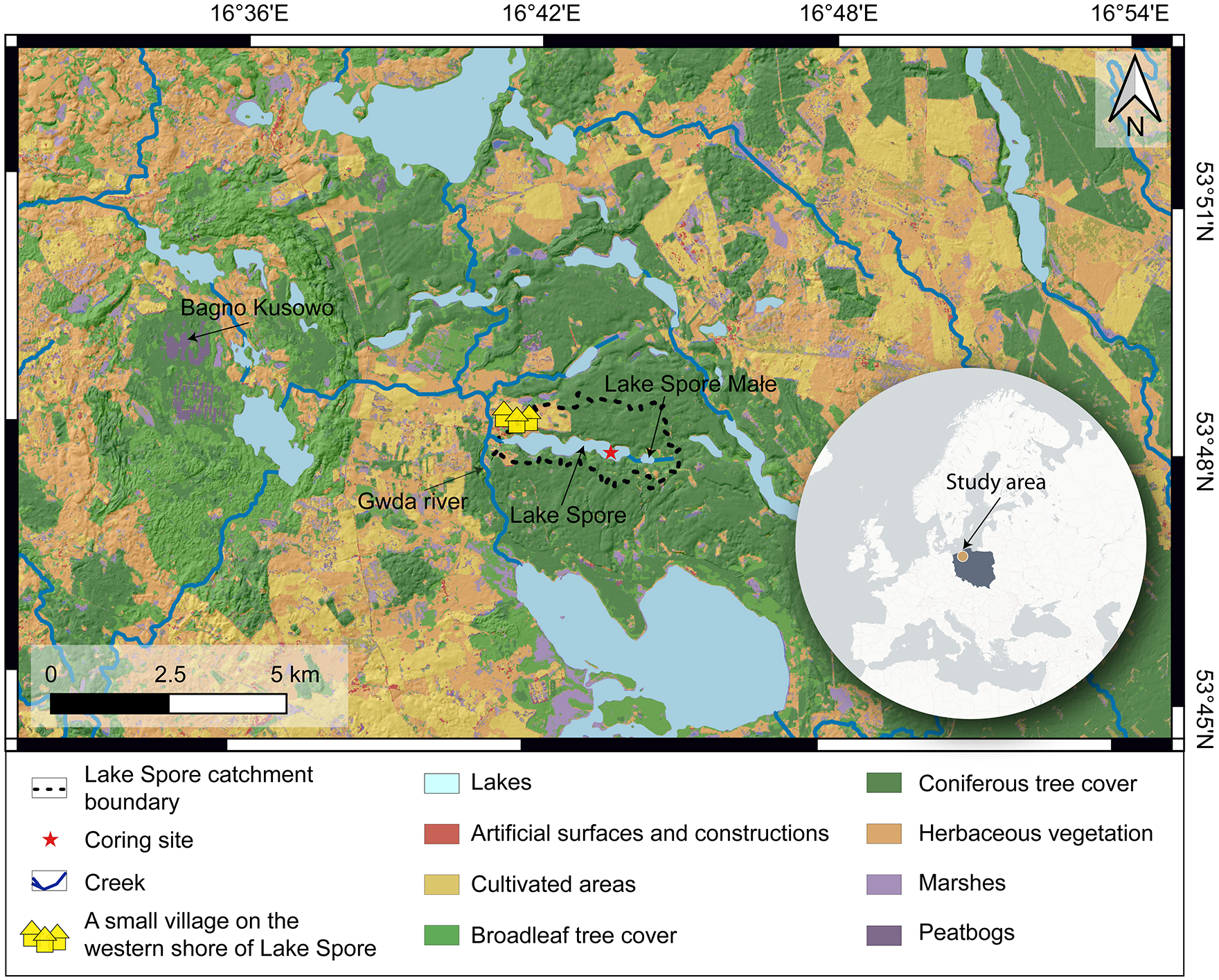
Location of Lake Spore within Europe, with Poland marked gray along with a land cover map of the direct vicinity of the lake based on CORINE land cover inventory.

Lake Spore is located in the central European climatic transition zone, which separates the mild and humid Atlantic climate of Western Europe from the continental climate of Eastern Europe. The total annual precipitation averages 753 mm, with the highest amount occurring during the summer months (Climate Data, 2021). The mean annual, July (the warmest month), and January (the coldest month) air temperatures are 8.5°C, 18.1°C, and −1.3°C, respectively (Climate Data, 2021).

The W-E elongated basin of Lake Spore covers approximately 85 ha and is shallow, with a maximum water depth of 7 m in the eastern part of the basin (Pleskot et al., 2020). Lake Spore is polymictic, well oxygenated, and slightly alkaline (pH ~8) (Pleskot et al., 2019) with a Ca concentration of 33.8 mg L⁻¹, as measured in summer 1989 (Jańczak, 1996). A 300 m-long creek connects Lake Spore to Lake Spore Małe (max. depth ~2.5 m; Figure 1). Lake Spore and Lake Spore Małe were a single water body before the development of wetlands between them ca. 3.4 kyr BP (Pleskot et al., 2020). While Lake Spore is drained to the west by the single stream that connects the lake to the Gwda River (Figure 1), neither Lake Spore nor Lake Spore Małe has any inflowing streams from outside the catchment, suggesting that groundwater is their main recharge source (Pleskot et al., 2020). The depth to the water table varies between less than 1 m in the low-lying areas adjacent to the lakes and between 2 and 5 m in the more distant areas (Kostecki, 2003). Given the low relief of the region and shallow water table depths in the area, the groundwater catchment of Lake Spore is likely much more extensive than the surficial catchment. However, the precise boundaries of the Lake Spore groundwater catchment are not known.

The paleolimnological data for Lake Spore used in this study have been partly published by Pleskot et al. (2020). The authors based their work on an analysis of the 450 cm long S1 sediment core collected from the deepest part of the lake (Figure 1). Their main focus was the period between 3.8 and 4.5 kyr BP (Supporting Information S1), for which an analysis of multiple proxies was conducted (chironomids, Cladocera, pollen and spores, δ¹³C_org, δ¹⁵N_org, δ¹⁸O_carb, δ¹³C_carb, total organic carbon/total nitrogen, Fe, S, and loss on ignition at 550°C and 950°C). The results for the remaining part of the core (i.e. <3.8 kyr BP) included only Fe, LOI550, and LOI950 analyses as well as dating. The Bayesian age-depth model for the core was calculated from 11 ¹⁴C AMS dates carried out on terrestrial plant macrofossils (Supporting Information S1; Pleskot et al., 2020). The model suggested that the mean accumulation rate in the sampled site of the lake was stable over the last 4.5 kyr BP, averaging 0.97 mm year⁻¹, except for a slump at ~4.15 kyr BP that resulted in an event-like deposition of 14 cm of sediment.

Materials and methods

Data sources

This study relies on a dataset consisting of newly acquired and previously published results (Pleskot et al., 2020). Specifically, to the already existing dataset derived from the samples analyzed for pollen and spores (n = 20), Cladocera (n = 20), δ¹³C_org (n = 20), δ¹⁵N_org (n = 20), TOC/N (n = 20), Fe (n = 110), LOI550 (n = 223), and LOI950 (n = 223), we added new pollen and spores (n = 89), Cladocera (n = 88), TOC/N (n = 89), δ¹³C_org (n = 88), and δ¹⁵N_org (n = 88) samples collected every 4 cm between depths of 1 and 357 cm.

Pollen and spores analysis was performed on the 1 cm³ bulk sediment samples that were deflocculated in warm 10% KOH, decalcified using 10% HCl and subjected to a minimum 24-h treatment with HF to remove silica. Next, acetolysis was carried out to remove organics (Berglund and Ralska-Jasiewiczowa, 1986). Using a compound microscope with 400× and 1000× magnifications, pollen and spores were identified and counted to a minimum sum of 500 arboreal pollen (AP) grains. Pollen grains and spores were identified with atlases and keys (Beug, 2004; Moore et al., 1991). The results of the palynological analysis were expressed as percentages calculated based on the ratio of an individual taxon to the total pollen sum, that is, the sum of AP and nonarboreal pollen (NAP), from which pollen of aquatic and wetland taxa, spores and non-pollen palynomorphs were excluded.

Cladocera were analyzed on 1 cm³ bulk samples processed according to the procedure presented by Frey (1986). The samples were heated in 10% KOH for 25 min, decalcified with 10% HCl, sieved through a 33-µm mesh with distilled water, and then topped to a volume of 10 mL in a scaled test tube. Before counting, the remains were dyed with glycerol-safranine and analyzed under a compound microscope (100−400× magnification). Each microscopic slide was prepared using a 0.1 mL volume of homogenized solution. Two to three microscopic slides were used for each sample to count a minimum of 200 individuals. The identification followed the keys of Flössner (2000) and Szeroczyńska and Sarmaja-Korjonen (2007).

Total organic carbon and total nitrogen (TOC and N) were determined using an Elemental Analyzer Vario MICRO Cube. Prior to the analysis, the 1-cm³ bulk samples were dried at 105°C, homogenized, and decalcified with 10% HCl. The TOC/N ratio was calculated on a molar basis. The analysis was performed in the Uranium-Series Laboratory at the Institute of Geological Sciences of the Polish Academy of Sciences in Warsaw, Poland.

δ¹³C_org and δ¹⁵N_org were analyzed from 1-cm³ air-dried, homogenized and decarbonated samples using an elemental analyzer linked in a continuous flow to an isotope-ratio mass spectrometer (Thermo Flash EA 1112HT, Thermo Delta V Advantage). The measured ratios of ¹³C/¹²C and ¹⁵N/¹⁴N were expressed as per mil (‰) deviations from V-PDB and AIR international standards, respectively. The analytical precision of the analyses was within 0.1‰ for the carbon isotopes and 0.3‰ for the nitrogen isotopes. Stable isotope analysis of organic matter fractions was carried out in the Stable Isotope Laboratory at the Institute of Geological Sciences of the Polish Academy of Sciences in Warsaw, Poland.

Data analysis

As pollen percentage values may underestimate the presence of herbs and therefore landscape openness, we applied the REVEALS model (Sugita, 2007) to reconstruct the openness from the pollen counts. This indicator was calculated by summarizing the reconstructed median share of all the herbaceous taxa (NAP) included in the modeling (Artemisia, Calluna vulgaris, Cyperaceae, Poaceae undiff., Plantago lanceolata, Rumex acetosa/acetosella type, Secale cereale, and the sum of remaining Cerealia pollen types). We used the Lagrangian stochastic model for pollen dispersal and applied pollen productivity estimates derived for the SW-Baltic study area (dataset PPE. MV2015; Theuerkauf et al., 2016). We set the lake diameter in the model at 600 m, which approximates the diameter of the circle with an area nearly equal that of Lake Spore. The model was applied with the REVEALSinR function from the DISQOVER package (Theuerkauf et al., 2016) in R version 3.6.3 (R Core Team, 2020).

Additional analytical techniques required preprocessing of the geochemical dataset. We calculated the CaCO₃ relative contribution from the LOI950 data by multiplying the LOI950 percent values from Pleskot et al. (2020) by 2.2576 (Heiri et al., 2001). LOI550, which was presumed to represent the percentage of organic matter (Heiri et al., 2001), and Fe data were log-transformed. As CaCO₃ and OM were analyzed at a resolution twice as high as that of the remaining geochemical proxies, we selected every second CaCO₃ and OM sample. The final geochemical dataset used for statistical analyses consisted of 108 observations for CaCO₃, OM, δ¹³C_org, δ¹⁵N_org, TOC/N, and Fe from consistent depths. Transformation of the geochemical data before statistical analyses depended on the method used, and a suitable description is provided separately in addition to the presentation of the methods. For the biotic dataset (pollen, phytoplankton identified by palynological analysis, and Cladocera), we used square-root transformation for each statistical analysis. Pollen taxa and Cladocera were retained in the statistical analyses if they occurred in at least two samples and had a maximum abundance of at least 2%. The requirement for phytoplankton was a maximum abundance of at least 1% and occurrence in not fewer than two samples.

Stratigraphically constrained cluster analysis (CONISS) was used to determine the time of significant compositional changes in our records. This method constrains the clustering algorithm so that the resulting dendrogram joins only those samples that are adjacent by a sediment core depth. The analysis was performed separately for terrestrial vegetation (NAP and AP taxa along with reconstruction of vegetation openness derived from the REVEALS model), phytoplankton, Cladocera, and geochemical data. The number of significant zones was assessed by the broken stick model (Bennett, 1996). The analysis was performed with the rioja package version 0.9–15.1 (Juggins, 2017) in R. Prior to CONISS analysis, geochemical data were standardized to zero mean and unit variance.

A principal curve (PrC) was estimated separately on AP, NAP, phytoplankton, Cladocera, and geochemical data to analyze compositional trends. The separate estimates of PrCs for AP and NAP were intended to determine differences in trajectories of the development of trees and herbaceous plant compositions. A PrC is a nonlinear curve fitted through data in multiple dimensions that is usually superior to commonly used methods such as principal component analysis in terms of the variance explained if there is a single dominant gradient in the data (De’ath, 1999; Simpson and Birks, 2012). The PrC was initialized using the first correspondence analysis axis and subsequently estimated by fitting smoothing splines to abundances of individual taxa or values of geochemical variables. We used analog package version 0.17-5 (Simpson and Oksanen, 2020) in R for the PrC estimates. Prior to the analysis, geochemical data were standardized to the range of 1–2, as positive values were required for calculations.

A series of partial redundancy analyses (pRDA; Ter Braak, 1994) were carried out to assess the influence of terrestrial vegetation composition between the major vegetation shifts on the aquatic biological and geochemical proxies. The major terrestrial vegetation shifts (MTVSs) were recognized based on the results of the CONISS analysis performed on the terrestrial vegetation data (NAP and AP taxa along with reconstruction of vegetation openness derived from the REVEALS model) and the PrC estimates for AP and NAP. We assumed that a MTVS occurred at this statistically significant transition between the CONISS pollen zones (PZs) that was concurrent with noticeable PrC shifts in either AP or NAP. The PZs grouped by the MTVSs were used in the pRDA models as nominal explanatory variables, whereas phytoplankton, Cladocera, and geochemical records were used as quantitative response variables. We also ran a separate model for terrestrial vegetation data (NAP and AP taxa along with reconstruction of vegetation openness derived from the REVEALS model) to quantitatively assess the relationship between the pollen zones between the MTVSs and the data from which the zonation was derived. Because of the strong temporal autocorrelation in stratigraphical data, we partialed out the statistical effects of age (Lotter and Birks, 2003). The statistical significance of the pRDA models was assessed by 999 Monte Carlo permutation tests. The analyses were performed with the vegan package ver. 2.5–6 (Oksanen et al., 2019) in R. Prior to the analysis, geochemical data were standardized to zero mean and unit variance.

Results

Pollen analysis, openness reconstruction, and major terrestrial vegetation shifts

A total of 96 pollen taxa were identified, of which 16 occurred in at least two samples and had a maximum abundance of at least 2%. According to the broken stick model, there were seven statistically significant pollen zones (PZ1-PZ7) that were derived from the CONISS analysis of arboreal (AP) and nonarboreal (NAP) pollen abundance data combined with openness reconstruction based on the REVEALS model (Figure 2; Supporting Information S2).

Figure 2.

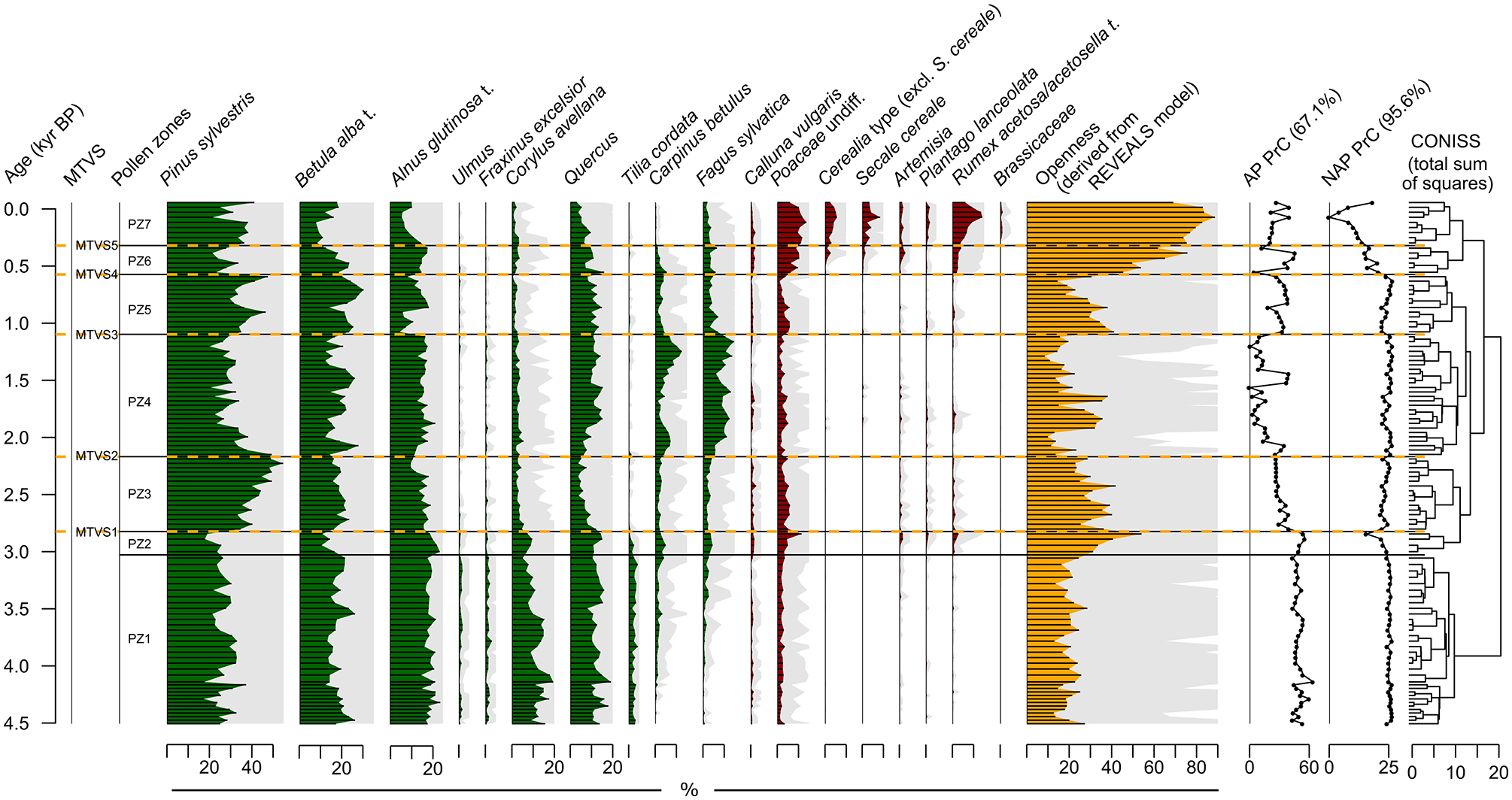
Pollen diagram of terrestrial vegetation. Percentages of tree taxa (AP) and herbaceous plants (NAP) are in green and red, respectively, whereas reconstruction of vegetation openness derived from the REVEALS model is in orange. The gray areas indicate values magnified by five. The numbers in parentheses above the AP and NAP PrC curves indicate the amount of variance explained by principal curves. The statistically significant pollen zones were distinguished based on the broken stick model applied to the results of CONISS analysis. Major terrestrial vegetation shifts (MTVSs) phases were set at these transitions between the statistically significant pollen zones that are concurrent with a noticeable change in either AP or NAP PrC values.

Within PZ1 (~4.55–3.03 kyr BP), Pinus sylvestris, Alnus glutinosa t. (hereafter t. = type), and Betula alba t. had the highest share among the tree taxa, with mean abundances of 27%, 19%, 18%, respectively. All herbaceous plants were characterized by low pollen counts, with the highest counts reported for Poaceae (up to 4%), which according to the REVEALS model constituted a major component of the open landscape (Supporting Information S2). Openness was relatively stable, with values rarely exceeding 20%.

The most noticeable change that occurred after the transition to PZ2 (~3.03–2.82 kyr BP) was a rise in openness that reached values up to 54% at the end of this zone and that resulted mainly from the increase in Poaceae (Supporting Information S2). The vegetation composition changed only slightly in this zone. We reported a higher relative contribution of A. glutinosa t., Corylus avellana, Fagus sylvatica, and Carpinus betulus and a lower share of P. sylvestris and B. alba t.

In PZ3 (2.82–2.17 kyr BP), P. sylvestris reached its highest abundance, with a mean of 40%. The pollen percentages of several deciduous tree taxa, including C. betulus, F. sylvatica, C. avellana, Quercus, and Tilia cordata, declined. Openness was relatively high, with values ranging between 22% and 42%.

PZ4 (2.17–1.10 kyr BP) revealed a decrease in P. sylvestris to values mostly below 30% and the highest pollen percentages of C. betulus and F. sylvatica in the entire profile (up to 13% and 15%, respectively). C. betulus revealed two maxima with distinct decreases in values at ~1.45–1.90 kyr BP. Openness was mostly <15% but rose noticeably between ~2.0 and 1.75 kyr BP, reaching up to 38%.

Following the transition to PZ5 (~1.10–0.57 kyr BP) P. sylvestris and B. alba t. increased their proportions (mean percentages: 37% and 24%, respectively), whereas C. betulus and F. sylvatica declined to values mostly <5%. Alnus glutinosa t. showed a drop from 17% to 5% at the transition from PZ4 to PZ5, but it regenerated at ~0.90 kyr BP. Openness increased at the onset of PZ5 to 41% due to the spread of Poaceae (Supporting Information S2) and then gradually decreased, reaching 15% at the termination of the zone.

In PZ6 (~0.57–0.32 kyr BP), the composition of herbaceous plants changed noticeably for the first time in the record. In addition to the increasing percentage of Poaceae undiff., we reported a higher Rumex acetosa/acetosella t. contribution and spread of Secale cereale and other cereals that gradually became a dominant component of the open landscape (Supporting Information S2). Openness increased sharply at the onset of the zone to 45% and then continued to rise to 62%. P. sylvestris declined (mean abundance of 26%), whereas the remaining AP taxa remained mostly stable.

PZ7 (<0.57 kyr BP) revealed a further increase in openness that reached its maximum (89%) at ~0.07 kyr BP. Most of the dominant NAP taxa reached their maximum values within PZ7. The share of most tree taxa mostly declined except for P. sylvestris, whose values fluctuated between 22% and 42%.

The PrC explained 67.1% of the variance for AP and 95.6% for NAP (Figure 2). High AP PrC values were associated with C. avellana and T. cordata, moderate values were associated with P. sylvestris, and low values were associated with F. sylvatica and C. betulus (Supporting Information S4). For NAP PrC, low values were associated primarily with R. acetosa/acetosella t., S. cereale, and other cereals (Supporting Information S5). Low and middle values were associated with Poaceae. No NAP taxa revealed a strong association with high PrC values. AP PrC values were high with small fluctuations within PZ1 and PZ2. At the transition to PZ3, PrC dropped to middle values that persisted up to PZ4. Then, the values dropped again and remained mostly low until the transition to PZ5, where another shift to middle values occurred. PZ6 and PZ7 revealed mostly moderate but fluctuating values. NAP PrC values were high with small fluctuations until the transition to PZ6. Then, NAP PrC values revealed a gradual decline that terminated at ~0.07 kyr BP, followed by PrC rebound to high values.

Given the criteria provided in the Materials and methods section, the transitions between PZs represented major terrestrial vegetation shifts (MTVSs), except for the transition from PZ1 to PZ2, which did not correspond to the substantial compositional change in AP and NAP depicted by the PrCs (Figure 2). Therefore, five MTVSs were indicated in our record, numbered from 1 to 5 (from the oldest to the youngest) delimited at ~2.82, 2.17, 1.10, 0.57, and 0.32 kyr BP (Figure 2).

Phytoplankton analysis

A total of 14 phytoplankton taxa were identified by palynological analysis, of which nine occurred in at least two samples and had a maximum abundance in a sample of at least 1%. Three significant phytoplankton CONISS zones were identified in the record (PhZ1-3).

In PhZ1 (4.55–2.13 kyr BP), of the algal species, Tetraëdron minimum and Scenedesmus ellipticus were the most abundant (mean percentages: 43% and 9%, respectively). Although the record revealed substantial fluctuations, the taxonomic composition was stable, and the only noticeable change was the slight increase in Pedistrum boryanum var. boryanum at ~2.82 kyr BP, that is, at MTVS1.

The transition to PhZ2 (~2.13–0.84 kyr BP) occurred immediately after MTVS2 (~2.17 kyr BP) and was associated with a noticeable decrease in the abundance of almost all the phytoplankton taxa. Of the species, T. minimum remained the most abundant, with a mean relative abundance of 16%.

In PhZ3, (<0.84 kyr BP) the contribution of T. minimum increased on average but fluctuated substantially (values ranged from 3% to 60%). The two-step rise was also reported for P. boryanum var. boryanum. The first rise occurred at the onset of the zone (from <6% to 11%), and the second (up to 40%) followed MTVS5 at ~0.32 kyr BP and was accompanied by the HdV-600 Aphanizomenon increase.

PrC explained 91.0% of the variance in the phytoplankton data (Figure 3). Low PrC values were associated with T. minimum and S. ellipticus, and high values were associated with P. boryanum var. boryanum (Supporting Information S6). Phytoplankton PrC values fluctuated substantially throughout the record. The PrC record can be divided into two parts with low values up to the transition from PhZ1 to PhZ2 (~2.13 kyr BP) and high values thereafter.

Figure 3.

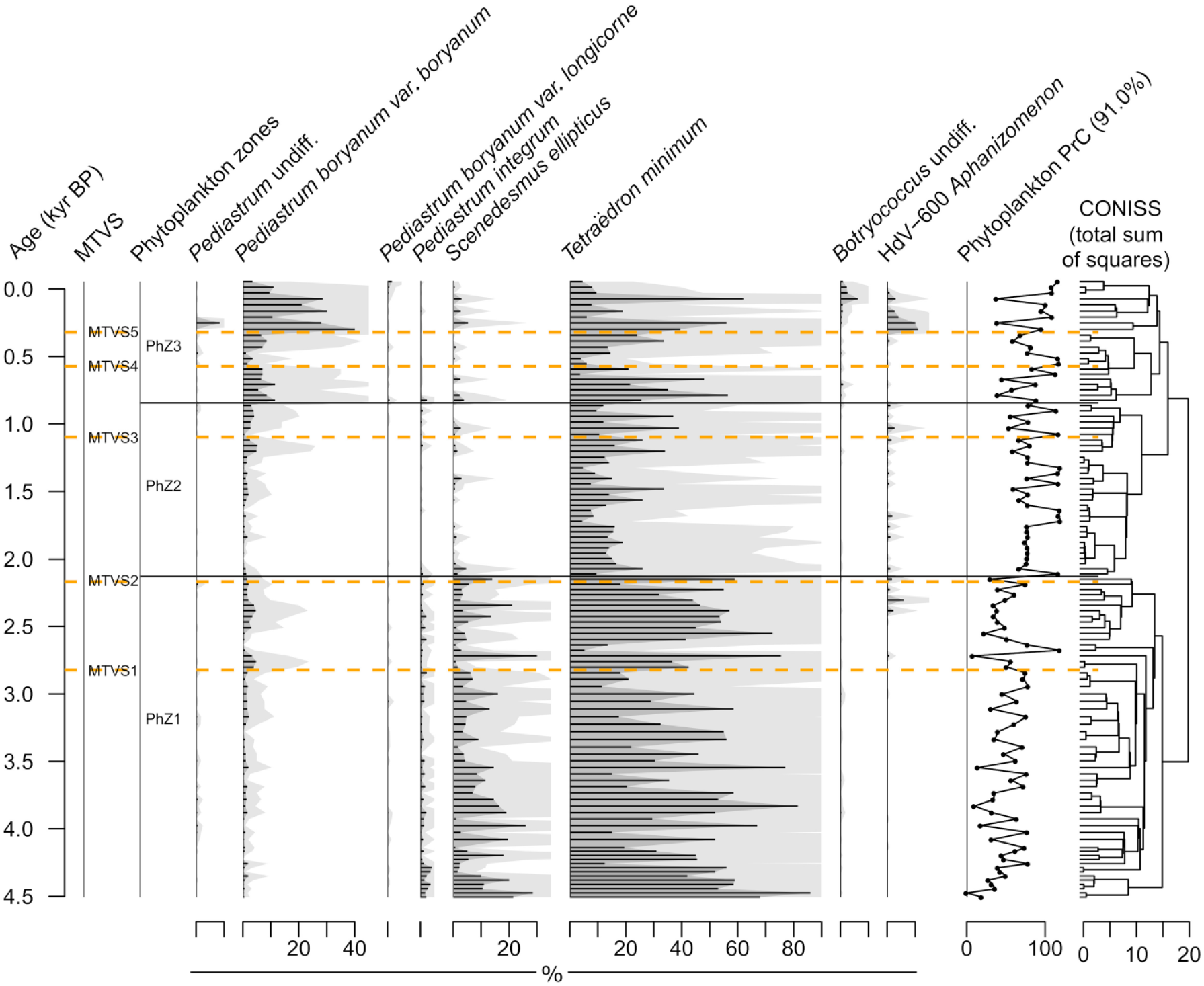
Percent diagram of phytoplankton taxa identified by the means of palynological analysis. Phytoplankton PrC estimates are also shown with the amount of variance explained by PrC provided in parentheses. The statistically significant phytoplankton zones were distinguished based on the broken stick model applied to the results of CONISS analysis. Major terrestrial vegetation shifts (MTVSs) were established based on the results of pollen analysis (see Figure 2 as well as the Materials and methods section for explanations).

Cladocera analysis

A total of 43 Cladocera taxa were identified, of which 33 occurred in at least two samples and had a maximum abundance of at least 2%. Cladocera abundance was generally stable below 15 k specimens cm⁻³ (Figure 4). The only two periods for which we reported noticeable variations and higher abundance of the fauna were at ~0.9–0.5 and after ~0.2 kyr BP. Four significant Cladocera CONISS zones were identified in the record (CZ1-4; Figure 4).

Figure 4.

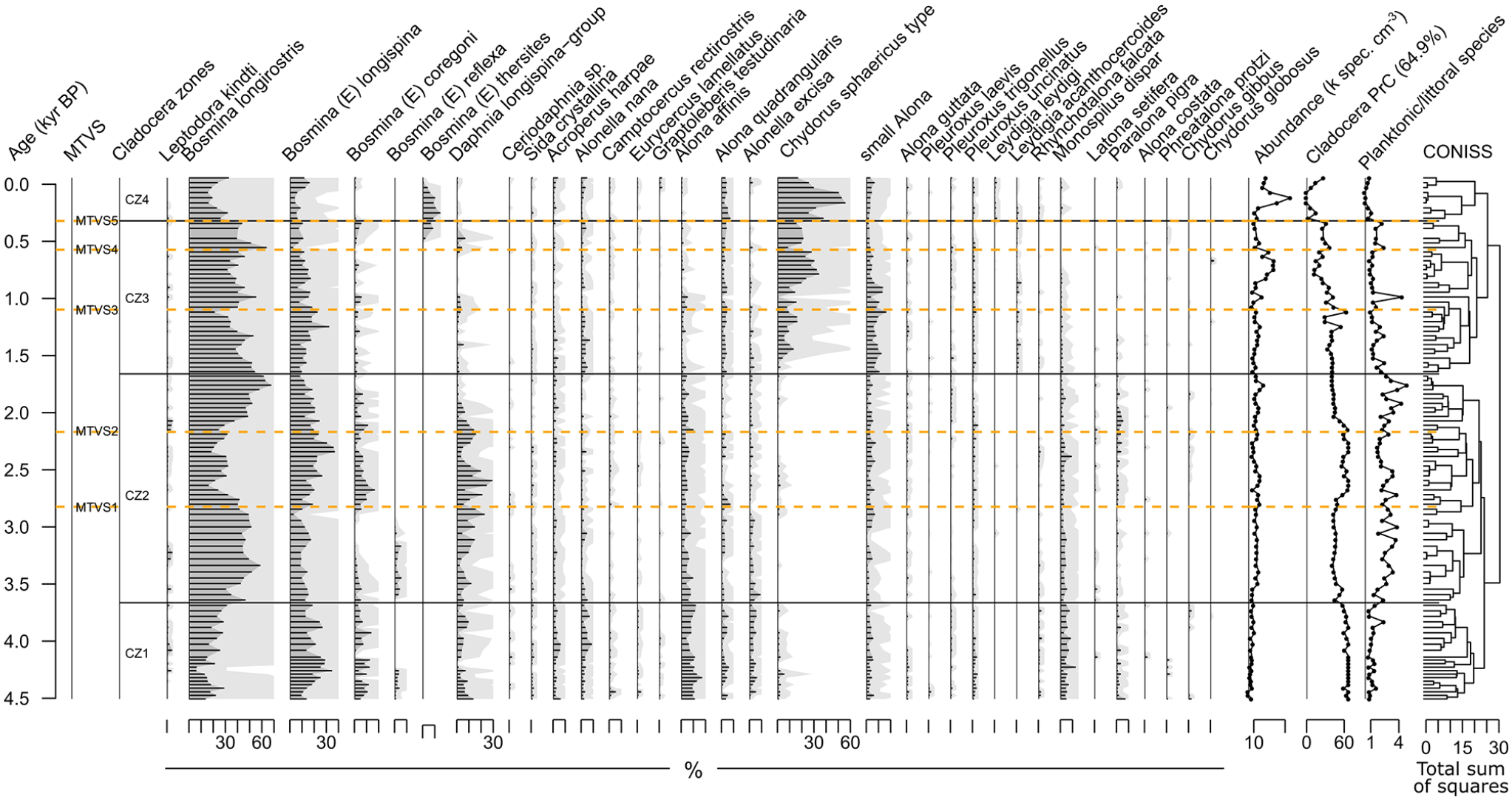
Percent diagram of Cladocera taxa along with total Cladocera abundance data and PrC estimates (amount of variance explained provided in parentheses). The statistically significant cladoceran zones were distinguished based on the broken stick model applied to the results of CONISS analysis. Major terrestrial vegetation shifts (MTVSs) were established based on the results of pollen analysis (see Figure 2 as well as the Materials and methods section for explanations).

Bosmina (E) longispina and Bosmina longirostris were the two dominant species (mean percentages: 20 and 19, respectively) in CZ1 (~4.55–3.66 kyr BP). A relatively high contribution was also reported for Alona affinis (4–17%) and Bosmina (E) coregoni (up to 14%). The planktonic to littoral species ratio (P/L) remained mostly stable at ~1.

In CZ2 (~3.66–1.66 kyr BP), the contributions of B. (E) longispina and B. longirostris remained high but fluctuated. A major shift in the contribution of these taxa occurred at MTVS1 and MTVS2 (~2.82 and 2.17 kyr BP). Between these MTVSs, the share of B. longirostris was on average 19% lower than that in the remaining part of CZ2, while the contribution of B. longispina was elevated (8% on average), as was the share of B. coregoni and the Daphnia longispina group. The P/L fluctuated but revealed higher values (mostly >2) in CZ2 than in the remaining part of the record.

In CZ3 (~1.66–0.32 kyr BP), the share of the Chydorous sphaericus type increased from near 0% to 34%. After 0.91 kyr BP, the contribution of this species exceeded that of B. longispina, of which the relative abundance did not change noticeably following the transition from CZ2. The contribution of B. longirostris remained high but fluctuated between 21% and 64%. We reported a noticeable change in Cladocera at MTVS4 (~0.57 kyr BP); namely, the contribution of the C. sphaericus type decreased by 9%, whereas that of B. longirostris increased by 19%. In CZ3, the P/L was mostly below 2, with a noticeable P/L rise occurring at ~1.0 kyr BP and between MTVS4 and MTVS5, that is, at ~0.57–0.32 kyr BP.

The transition to CZ4 (~0.32 kyr BP) was concurrent with MTVS5. The main change in the composition of Cladocera within CZ4 was a decline in B. longirostris to a mean relative abundance of 23% and an increase in the B. (E) thersites and C. sphaericus types (mean percentages in CZ4: 7 and 36, respectively). The latter taxon became the most abundant among the Cladocera. The P/L values were the lowest in the entire profile (<1).

The PrC explained 64.9% of the variance for the Cladocera data (Figure 4). Low PrC values were primarily associated with C. sphaericus type and B. thersites, middle values with B. longirostris and small Alona, and high values with A. affinis, B. (E) coregoni, D. longispina-group, B. (E) longispina, and Monospilus dispar (Supporting Information S7). Overall, PrC values decreased toward the top of the core. However, three noticeable positive excursions occurred at 2.75–2.10, 0.57–0.32, and >0.05 kyr BP. The change in PrC values at 0.57–0.32 kyr BP matched MTVS4 and MTVS5, whereas the change at 2.75–2.10 was slightly delayed in comparison with MTVS1 and MTVS2.

Geochemical analysis

Eight significant geochemical CONISS zones were identified (GZ1-8). The transitions between GZ1 (~4.55–4.24 kyr BP) and GZ2 (~4.24–4.11 kyr BP) as well as GZ2 and GZ3 (~4.11–2.82 kyr BP) revealed substantial variability in the geochemical record. As this part of the record was presented in detail by Pleskot et al. (2020), we do not provide its description here.

In GZ3 and GZ4 (~2.82–0.97 kyr BP), the geochemical record was mostly stable, with CaCO₃ relative contributions markedly higher than those of OM (64 vs 16 of mean percentages), Fe concentrations ranging from 12 to 33 g kg⁻¹, and TOC/N values fluctuating approximately 13. δ¹³C and δ¹⁵N records had mean values of −31.0‰ and −0.6‰, respectively. The most notable changes over GZ3 and GZ4 included a slight increase in Fe and OM accompanied by a slight decrease in CaCO₃ between MTVS1 (~2.82 kyr BP) and MTVS2 (~2.17 kyr BP).

In GZ5 (~0.97–0.45 kyr BP), most geochemical variables remained stable except for a two-step rise in Fe. The first rise in Fe (from 20 to 23 g kg⁻¹) was reported at the onset of GZ5, which lagged MTVS3 for 130 years, whereas the second Fe rise (up to 33 g kg⁻¹) occurred at ~0.57 kyr BP, that is, synchronously with MTVS4.

The last three geochemical zones, namely, GZ6 (~0.45–0.32 kyr BP), GZ7 (~0.32–0.10 kyr BP), and GZ8 (~0.10–0.07 kyr BP), were characterized by substantial compositional turnover in our geochemical dataset. δ¹³C and δ¹⁵N revealed sharp increases (from −31.7‰ to −29.5‰ and from −1.7‰ to 0.6‰, respectively) at the transition to GZ6 and further increases at the transition to GZ7 that corresponded to MTVS5 (~0.32 kyr BP). The values of the stable isotopes remained high to the present. CaCO₃ decreased gradually from the late part of GZ5, when MTVS4 occurred, toward the top, reaching its minimum (3%) after the transition to GZ8. OM and TOC/N increased sharply at the transition to GZ6 but returned to lower values at the shift to GZ7. Following the transition to GZ8, OM increased sharply again, reaching its maximum (49%) at the top of the record, whereas TOC/N remained low, with a mean value of 11. Fe decreased sharply at the transition to GZ6 to the lowest values in the entire record (11 g kg⁻¹) and rebounded partly following the transition to GZ8.

The PrC explained 86.9% of the variance in the geochemical data (Figure 5). Low PrC values were associated with δ¹³C, δ¹⁵N, and OM; moderate and high values were associated with TOC/N; and high values were associated with CaCO₃ (Supporting Information S8). In GZ1, PrC values were high but increased further in GZ2. Following the transition to GZ3, PrC values decreased but remained high and stable up to the transition to GZ6. Afterward, the PrC curve decreased gradually, reaching minimum values at the top of the record.

Partial redundancy analysis

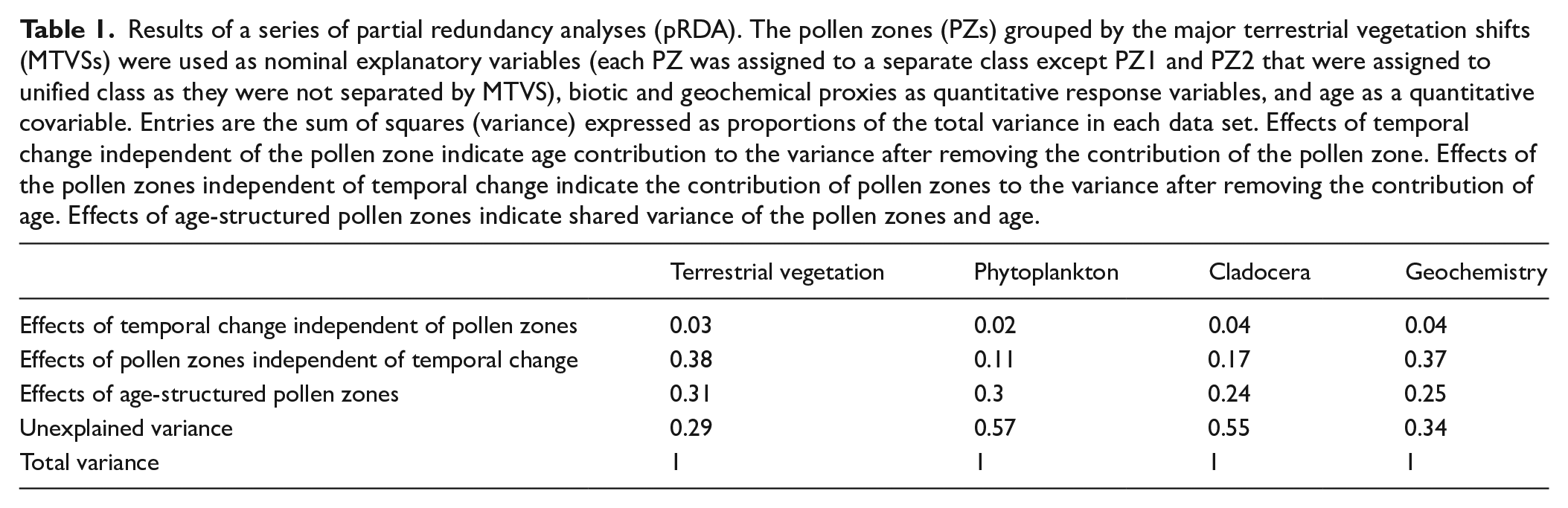
In the partial redundancy analysis, each PZ was assigned to a separate class of nominal explanatory variables except for PZ1 and PZ2, which were assigned to a unified class as they were not separated by MTVS. The analyses produced statistically significant models for all our data subsets. The highest proportion of variance explained by the vegetation composition between the MTVSs was reported for terrestrial vegetation (0.38) and geochemistry (0.37; Table 1), whereas for Cladocera and phytoplankton data, the proportion of variance explained was 0.17 and 0.11, respectively. When vegetation composition was considered in conjunction with age, the proportion of variance explained increased markedly in the models, whereas when the effects of the temporal change were considered independent of vegetation composition, the variance explained was low and did not exceed 0.04 (Table 1). The proportion of variance unexplained by temporal change and vegetation composition was high for phytoplankton and Cladocera (0.57 and 0.55, respectively) and noticeably lower for geochemistry and terrestrial vegetation data (0.34 and 0.29, respectively).

Table 1.

Results of a series of partial redundancy analyses (pRDA). The pollen zones (PZs) grouped by the major terrestrial vegetation shifts (MTVSs) were used as nominal explanatory variables (each PZ was assigned to a separate class except PZ1 and PZ2 that were assigned to unified class as they were not separated by MTVS), biotic and geochemical proxies as quantitative response variables, and age as a quantitative covariable. Entries are the sum of squares (variance) expressed as proportions of the total variance in each data set. Effects of temporal change independent of the pollen zone indicate age contribution to the variance after removing the contribution of the pollen zone. Effects of the pollen zones independent of temporal change indicate the contribution of pollen zones to the variance after removing the contribution of age. Effects of age-structured pollen zones indicate shared variance of the pollen zones and age.

	Terrestrial vegetation	Phytoplankton	Cladocera	Geochemistry
Effects of temporal change independent of pollen zones	0.03	0.02	0.04	0.04
Effects of pollen zones independent of temporal change	0.38	0.11	0.17	0.37
Effects of age-structured pollen zones	0.31	0.3	0.24	0.25
Unexplained variance	0.29	0.57	0.55	0.34
Total variance	1	1	1	1

Discussion

Drivers and spatial extent of major vegetation shifts recognized in the Lake Spore record

Of the five major terrestrial vegetation shifts (MTVSs) recognized in this study, four were concurrent with or closely followed a sharp rise in landscape openness (MTVS1 and MTVS3-5; Figures 2 and 6). The map of potential vegetation surrounding Lake Spore, that is, the vegetation which would most likely cover the area if humans had not interfered, does not reveal any large-scale open vegetation stands (Matuszkiewicz et al., 1995). Thus, the abrupt and persistent openness rise at the MTVSs suggests that the declines in forest cover most likely resulted from human-induced deforestation, making anthropogenic factors a major driver of landscape transformation in the study area over the late-Holocene. This finding confirms the conclusion drawn from previous studies that vegetation composition and dynamics in Poland during the late-Holocene were controlled to a large extent by human impacts (Ralska-Jasiewiczowa et al., 2003; Starkel et al., 2013). As suggested by Pędziszewska et al. (2015), deforestations in northern Poland were conducted mainly with the use of fire until at least the early medieval times. The spread of fire in the area could have been facilitated by the high contribution of fire-prone Pinus sylvestris and frequently occurring summer droughts (Pędziszewska et al., 2015).

Although the dominant role of anthropogenic factors in the local landscape transformation over the recent millennia appears undeniable, the influence of other drivers cannot be neglected. The most notable example of regional vegetation change to which human impact contributed to a limited extent is the MTVS2. The shift resulted primarily from the spread of Carpinus betulus and Fagus sylvatica. Both tree species were late immigrants that started to spread to the studied area ~4 kyr BP (Ralska-Jasiewiczowa et al., 2003). The onset of their substantial contribution to the forests of western Poland at ~2 kyr BP is well documented (Ralska-Jasiewiczowa et al., 2003). In the area adjacent to Lake Spore, this change in vegetation composition was ascribed to economic decline and associated forest regeneration that followed the rapid expansion of pastures, grasslands, and cultivated fields during the early phase of Iron Age between 2.75 and 2.27 kyr BP (Pędziszewska et al., 2015).

We argue that natural processes could also have contributed substantially to P. sylvestris spread at MTVS1 (~2.82 kyr BP) and Alnus retreat at MTVS3 (~1.10 kyr BP). The unprecedented spread of opportunistic P. sylvestris at 2.82 kyr BP, even if primarily favored by local deforestation, could have been reinforced by a drier climate at the Homeric Minimum in Poland at that time (Słowiński et al., 2016), which provided unfavorable conditions for the regeneration of more demanding tree species. According to Latałowa et al. (2019), the Alnus decline at approximately 1.10 kyr BP was a widespread event in the Polish lowlands and adjacent areas and was linked to a pathogen outbreak favored by the preceding series of climatic extremes. This event noticeably affected the structure of the forest surrounding Lake Spore, as pollen data revealed that percentages of A. glutinosa type declined from ~20% to less than 10% for approximately 200 years.

The vegetation changes reconstructed in our work closely match the results of Lamentowicz et al. (2015) that were derived from pollen analysis of the peat core extracted from the nearby (~7 km) Bagno Kusowo in terms of the trajectory of vegetation development and ages of the most prominent vegetation turnovers. This result suggests that none of the vegetation shifts around Lake Spore were site-specific events. Moreover, apart from the already mentioned region-wide distinct spread of C. betulus and F. sylvatica prior to 2 kyr BP, we found another two events analogous to the MTVSs identified in our record that were reported from more distant sites than Bagno Kusowo. The first event was an expansion of P. sylvestris at ~2.82 kyr BP, and the second was a retreat of F. sylvatica and C. betulus at ~0.57 kyr BP. Both events were recorded in Lake Skrzynka and Lake Suminko, which are located 55 and 75 km from the study site, respectively (Apolinarska et al., 2012; Pędziszewska et al., 2015). Consequently, it is very likely that of the five MTVSs we recognized in our record, at least three (at ~0.57, 2.17, 2.82 kyr BP) not only extended beyond the direct vicinity of Lake Spore, as evidenced by a very similar pollen record from Bagno Kusowo, but also were synchronous with the vegetation change that occurred on a regional scale.

Although the share of open land within the range of 10 km from Lake Spore is currently relatively high (Figure 1), the direct vicinity of a major part of the lake is covered with forest. The persistence of forest cover in the areas directly adjacent to Lake Spore could have been common even during the major phases of local forest clearings in the past, as indicated by the TOC/N curve that records variations in the organic carbon source to the lake sediments (Meyers and Ishiwatari, 1993). According to Kaushal and Binford (1999), the periods of catchment deforestations are followed by the enhanced supply of terrestrial organic matter to lakes and the associated rise in lake sediment TOC/N values. Although the Lake Spore TOC/N record showed several positive excursions, its overall trend was mostly stable up to ~0.45 kyr BP (Figure 5). The only prolonged period of the enhanced supply of terrestrial organic matter that could have been associated with deforestation of the lake’s shores occurred between ~0.32 and 0.45 kyr BP (GZ6), as indicated by the markedly higher values of TOC/N at that time. It is, however, important to note that TOC/N likely revealed variations in the supply of terrestrial organic carbon derived mainly from the eastern part of the catchment. In turn, the transport of particulate organic matter from the west to the coring location was hampered by noticeable shallowing in the middle part of the lake basin (Pleskot et al., 2020), which itself is noticeably elongated in the W-E direction. Therefore, we cannot exclude the possibility that the eastern shores of Lake Spore experienced more prolonged periods of forest clearance.

Figure 5.

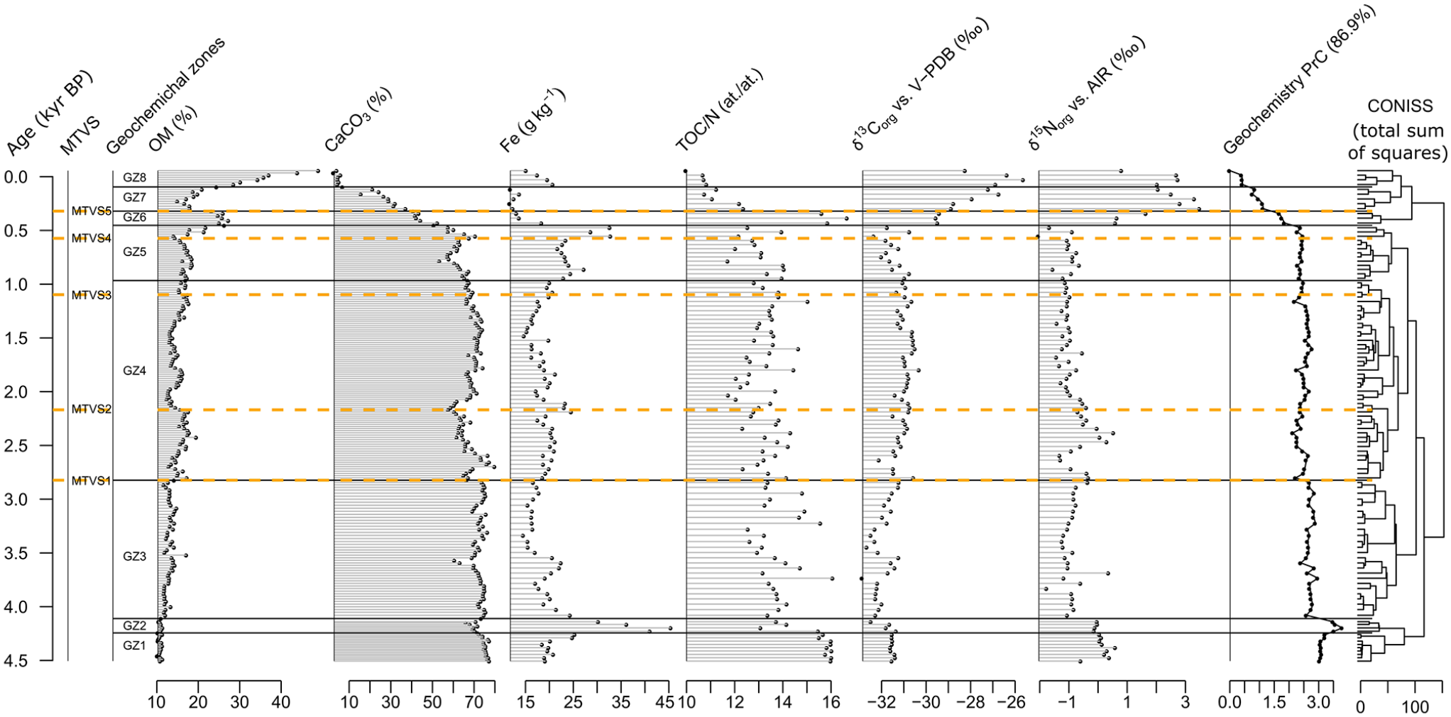
Geochemical data along with PrC estimates (amount of variance explained provided in parentheses). The statistically significant geochemical zones were distinguished based on the broken stick model applied to the results of CONISS analysis. Major terrestrial vegetation shifts (MTVSs) were established based on the results of pollen analysis (see Figure 2 as well as the Materials and methods section for explanations).

Effects of MTVSs on the lake environment

We found that MTVSs were concurrent with several noticeable compositional turnovers in our proxy records (Figure 6), suggesting that the influence of terrestrial vegetation dynamics on the lake environment was substantial. This result was further confirmed by pRDA. We found that the pRDA models produced for phytoplankton, Cladocera, and geochemical data were all statistically significant when subsequent pollen zones (PZs) separated by MTVSs were used as nominal explanatory variables (Table 1). Moreover, the variance explained was noticeable for each dataset even when the influence of age was partialed out. Such a result of the pRDA confirms the association of our proxy records with vegetation type between the MTVSs. Overall, our findings are consistent with the results of several other studies reporting the substantial influence of terrestrial vegetation dynamics on lake ecosystems over long temporal scales (Engels, 2021; Mariani et al., 2018; Puusepp and Kangur, 2010). The MTVS effects on Lake Spore were variable and could have included impacts on lake productivity, chemistry, and water levels (Figure 6). However, not all the shifts in our dataset corresponding to MTVSs could be readily explained by these impacts.

Figure 6.

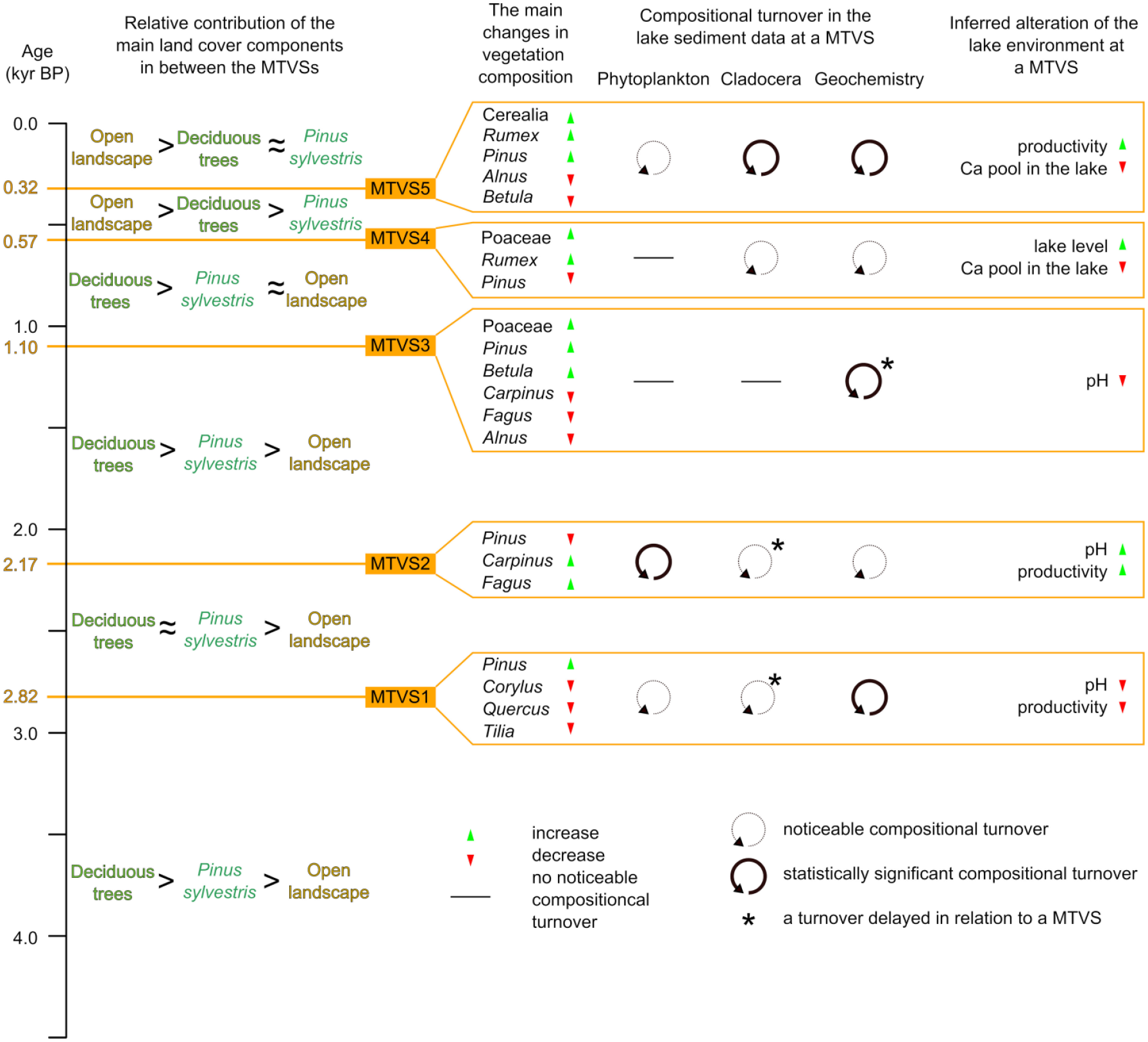
Summary figure showing the main changes to vegetation composition at the major terrestrial vegetation shifts (MTVSs), the extent of changes in the lake sediment record concurrent to MTVSs, and our interpretation of the lake ecosystem response to the vegetation shifts.

Trophic status

We reported that the clearest change in Lake Spore trophic status was concurrent with the MTVS at ~0.32 kyr BP (MTVS5), as recorded primarily by rising values of productivity proxies such as δ¹⁵N and δ¹³C (Figure 5) as well as the expansion of several species associated with eutrophic conditions, such as Chydorus sphaericus type, Pediastrum boryanum var. boryanum, or HdV-600 Aphanizomenon (Figures 3 and 4). We argue that the impact of the changes in terrestrial vegetation on nutrient supply to the lake is unlikely to fully explain the shift in the lake’s trophic status. The additional factor that could have played a role was the enhancement of internal nutrient loading due to the intense wind-induced mixing of the water column associated with the highest degree of landscape openness following MTVS5 during the entire late-Holocene history of the area (Figure 2). However, such a sharp rise in lake productivity from internal nutrient loading would not be possible without deforestation of the lake shores that we described in the previous section and that preceded MTVS5 for over 100 years. Deforestation can substantially increase the input of dissolved nutrients and particulate matter to aquatic ecosystems by increasing the runoff from the catchment (Bormann et al., 1974; Bradshaw et al., 2005). In our record, the enhanced nutrient supply to the lake prior to MTVS5 was indicated by the initial increase in the δ¹⁵N and δ¹³C values corresponding to the TOC/N positive excursion between 0.32 and 0.45 kyr BP (Figure 5). Additionally, the eutrophication of the lake following MTVS5 could have been influenced by the enhanced nutrient supply to the lake from the use of fertilizers for the cultivation of cereals, the contribution of which has risen substantially in our pollen record since 0.32 kyr BP. However, the role of soil fertilization practices in increasing lake productivity was probably not essential at MTVS5, as nutrient-rich synthetic fertilizers that are capable of markedly influencing lake trophic status (Poraj-Górska et al., 2017) were introduced in northern Poland only in the 20th century (Gorzelak, 2011).

Shifts in lake productivity were less clear but plausible for MTVS1 (~2.82 kyr BP) and MTVS2 (~2.17 kyr BP) and were not recorded for MTVS3 (~1.10 kyr BP) and MTVS4 (~0.57 kyr BP; Figures 5 and 6). The change in Lake Spore trophic status at MTVS1 and MTVS2 can be inferred from the Cladocera data that show a Bosmina longirostris decline at MTVS1 accompanied by a rise of B. longispina and B. coregoni and the opposite at MTVS2. Replacement of B. longirostris by Eubosminas (B. (E) longispina and B. (E) coregoni) is commonly associated with productivity fluctuations, with periods of higher B. longirostris contributions indicating more productive lake waters (Adamczuk, 2016), suggesting that MTVS1 could have been followed by a decrease in lake trophic status, whereas MTVS2 could have been followed by lake eutrophication. We argue that these trophic status shifts could have been a consequence of alterations in humus composition and thus terrestrial nutrient cycling following MTVSs. The main change at the vegetation shifts was a spread (MTVS1) and subsequent retreat (MTVS2) of P. sylvestris (Figure 2). The presence of this tree species favors the formation of mor humus, which differs markedly from mull/moder forms of humus occurring under deciduous tree canopies in terms of nutrient cycling (Ponge, 2003). Although trophic shifts in Lake Spore following humus transformations appear likely, they were not confirmed by the isotopic data that suggest no noticeable change at MTVS1 and MTVS2 (Figure 5). Therefore, we cannot exclude the possibility that the composition of Cladocera at these two shifts was driven by factors other than productivity changes.

Lake chemistry

A distinct yet gradual decline in CaCO₃ following MTVS4 and MTVS5 (Figure 5) likely recorded the most notable change in the lake chemistry associated with MTVSs that could have resulted from a substantial reorganization of the catchment Ca cycle. The surficial sediments around Lake Spore are dominated by fluvioglacial sands containing a small amount of carbonates (Popielski, 2006), which are known to provide the main source of Ca ions to aquatic ecosystems in young glacial landscapes of Polish lowlands (Bukowska-Jania and Pulina, 1999). Consequently, any disturbance to Ca leaching rates can result in a concentration of the element in recipient lake waters that is not high enough for abundant calcite precipitation. Since tree species are generally much more efficient in soil Ca absorption and thus in the incorporation of Ca into the catchment element cycle than grasses (Jobbágy and Jackson, 2004), one can expect a gradual decline in the supply of this element to lakes following major deforestation. This is particularly true if the rise in landscape openness is persistent over a long period of time. Thus, the explanation that the decline in CaCO₃ content over the last 570 years in Lake Spore resulted from the decline in Ca supply following widespread and persistent landscape deforestation appears plausible. Such an interpretation is further supported by the present-day characteristics of Lake Spore waters in terms of Ca concentration and pH, the latter being another crucial variable controlling CaCO₃ precipitation within lakes (Kelts and Hsü, 1978). Although the pH value in the lake (~8; Jańczak, 1996; Pleskot et al., 2019) is similar to that reported in Polish lakes within which abundant deposition of CaCO₃ occurs at present (Apolinarska et al., 2020; Bonk et al., 2015), the concentration of Ca (<34 mg L⁻¹; Jańczak, 1996) is two times smaller than that in other Polish lakes, suggesting it to be the main limiting factor for calcite precipitation within Lake Spore.

An alternating rise and decline in P. sylvestris at MTVS1 (~2.82 kyr BP) to MTVS3 (~1.10 kyr BP; Figure 6) could have resulted in yet another change to the lake’s chemistry. We found that a high (low) share of P. sylvestris between these shifts (Figure 2) was associated with high (low) sedimentary Fe content and slightly lower (higher) relative abundance of CaCO₃ (Figure 5). It is generally well known that P. sylvestris needles favor soil acidification and enhanced Fe leaching (Augusto et al., 2002; Bloomfield, 1953). Thus, it is likely that at the time when P. sylvestris reached a high abundance following MTVS1 and MTVS3, the lake was receiving more acidic waters enriched in ferrous iron. The acidification of lake water during the periods of P. sylvestris spread were inferred from the corresponding CaCO₃ decreases that likely marked the phases of less effective carbonate precipitation expected during the time of lower pH, whereas the concurrent increases in Fe likely followed the more efficient supply of iron from the lake catchment. The pH of the lake waters probably decreased only slightly due to the spread of P. sylvestris, as the relative contribution of carbonates to sediments remained high (~60%) even following declines.

Lake level

The lake level fluctuations were reconstructed to some extent based on the cladoceran planktonic/littoral (P/L) record (Figure 4), which is an acknowledged indicator of past water depth changes in lakes (Hofmann, 1998). Terrestrial vegetation turnover influence lake levels mainly through an associated change in catchment evapotranspiration rates that affects a catchment water budget (Dearing, 1997). However, of the five MTVSs, only two were concurrent with noticeable P/L shifts, namely, MTVS4 (~0.57 kyr BP) and MTVS5 (~0.32 kyr BP). The P/L increase at MTVS4 suggests a rise in the lake level that can be interpreted as the effect of the sharpest increase in landscape openness in the entire record at that time. This is because a distinct decrease in tree cover could have contributed to markedly lower water losses in the area through evapotranspiration and thus likely resulted in the rise of the groundwater table (Jackson et al., 2000). The lake level rise at MTVS4 was also favored by the climate, as suggested by the groundwater rise at the nearby Bagno Kusowo ombrotrophic bog after ~0.7 kyr BP and the concurrent shift toward cooler conditions in northern Poland (Lamentowicz et al., 2015; Pleskot et al., 2022). The inferences of lake level changes at MTVS5 based on P/L need to be carefully considered because of the distinct productivity increase at that time. Thus, even if the lake depth changed at MTVS5, neither the direction nor amplitude of this variation was likely to be reliably deduced from the Cladocera composition, which is expected to respond primarily to the trophic status shift.

Undifferentiated effects

Although it was possible to indicate likely drivers of some shifts in our data concurrent with MTVSs as described above, the mechanisms behind other shifts remained unclear, including the sharp and short-lasting decline in OM at MTVS5 (Figure 5), the positive excursion of Fe content at MTVS4 (Figure 5) or the major turnover in phytoplankton composition at MTVS2 (Figure 3). However, the synchronicity of these shifts with the MTVSs suggests that they could have been associated with vegetation turnover. Therefore, the summary of Lake Spore responses to the MTVSs presented in Figure 6 likely only partly reflects the influence of vegetation shifts on the lake ecosystem.

Relative importance of MTVSs to long-term lake ecosystem change

Although it is beyond the scope of this work to discuss the impact of drivers other than MTVSs on our record in detail, the impact clearly varies depending on the proxy considered. Our pRDA models indicate that the vegetation composition between the MTVSs explained almost the same proportion of variance in geochemical and pollen data (Table 1), suggesting that the terrestrial vegetation and the geochemical record were particularly related. The lower proportion of variance explained in phytoplankton and Cladocera data by the vegetation composition indicates a noticeable impact of drivers independent of MTVSs. For instance, it is likely that the major change in Cladocera composition between MTVS2 and MTVS3 marked by the gradual expansion of small-bodied taxa, in particular, the C. sphaericus type concurrent with a decline in the large-bodied cladocerans, such as the B. (E) longispina group (Figure 4), resulted from predation pressure from fishes (Nevalainen et al., 2015). However, despite these effects, the impact of MTVSs on both Cladocera and phytoplankton records remained clearly discernible. Consequently, MTVSs should be considered a major driver of the composition of these organisms over long temporal scales.

Summary and conclusions

The multiproxy analysis of the sediment core collected from Lake Spore, northern Poland, enabled us to reconstruct the responses of the lake to the major terrestrial vegetation shifts (MTVSs) in the late-Holocene. Our record revealed five MTVSs in the area adjacent to Lake Spore at ~0.32, 0.57, 1.10, 2.17, and 2.82 kyr BP. The main changes at the shifts included substantial landscape openness variations and altering proportions between Pinus sylvestris and deciduous trees. We found that vegetation dynamics at the study site were driven primarily by human-induced deforestation that was mostly distant from the lake shores.

Each MTVS was concurrent with a noticeable Lake Spore ecosystem change (Figure 6). The most noticeable change to the lake trophic status was a sharp productivity rise following MTVS5 (~0.32 kyr BP). We suggest that eutrophication was primarily associated with internal nutrient loading driven by enhanced wind-induced mixing of the water column following a sharp increase in openness. Less pronounced trophic state shifts could have also occurred following MTVS1 (~2.82 kyr BP) and MTVS2 (~2.17 kyr BP). Given that a substantial shift in the proportion of P. sylvestris and deciduous trees occurred at these MTVSs, it appears likely that humus composition and thus nutrient cycling were altered as well. However, although Cladocera data support trophic status changes at MTVS1 and MTVS2, they were not discernible from geochemical data.

The most prominent change to lake chemistry was a substantial depletion of the water calcium pool that could have resulted from a substantial reorganization of the catchment Ca cycle following the transition from a tree-dominated to a herb-dominated landscape that occurred at MTVS4 (~0.57 kyr BP) and continued after MTVS5 (~0.32 kyr BP). We also found slight changes in lake water pH and Fe content concurrent with shifting proportions between P. sylvestris and deciduous trees. Specifically, the higher contribution of P. sylvestris following MTVS1 (~2.82 kyr BP) and MTVS3 (~1.10 kyr BP) was associated with lower pH and higher Fe content, likely due to the soil acidification and enhanced iron leaching driven by P. sylvestris needles.

Although major changes in terrestrial vegetation composition are known to cause lake-level fluctuations, the only clear water depth change concurrent with an MTVS was a lake level rise recorded at ~0.57 kyr BP. We attribute this change to the large-scale deforestation that could have influenced the catchment water budget by decreasing evapotranspiration.

We found several noticeable compositional turnovers in our dataset concurrent with the MTVSs that were not easily interpretable. However, the synchronicity of these turnovers and MTVSs suggests that a causal relationship is plausible. The most noticeable turnover at an MTVS lacking a simple explanation was the distinct decline in several phytoplankton species following the establishment of the forest with the high contribution of Carpinus betulus and Fagus sylvatica at ~2.17 kyr BP.

Overall, our results show that MTVSs are of utmost importance to the long-term Lake Spore ecosystem changes. This finding stresses the need for greater appreciation of the importance of past vegetation dynamics in paleolimnological studies. Additionally, the results show that future changes in vegetation composition in lake catchments, if substantial, will likely markedly reinforce the direct stress on lake ecosystems exerted by climate change and human impacts.

Supplemental Material

sj-docx-1-hol-10.1177_09596836221088228 – Supplemental material for Responses of a shallow temperate lake ecosystem to major late-Holocene terrestrial vegetation shifts

Supplemental material, sj-docx-1-hol-10.1177_09596836221088228 for Responses of a shallow temperate lake ecosystem to major late-Holocene terrestrial vegetation shifts by Krzysztof Pleskot, Magdalena Suchora, Karina Apolinarska and Piotr Kołaczek in The Holocene

Footnotes

Acknowledgements

We thank two anonymous reviewers for comments that markedly improved the quality of the manuscript.

Funding

The author(s) disclosed receipt of the following financial support for the research, authorship, and/or publication of this article: The study was financed through a grant from the National Science Centre (NCN), Grant No. 2016/21/N/ST10/00313.

ORCID iDs

Krzysztof Pleskot

Karina Apolinarska

Piotr Kołaczek

Supplemental material

Supplemental material for this article is available online.

References

Adamczuk

(2016) Past, present, and future roles of small cladoceran Bosmina longirostris (O. F. Müller, 1785) in aquatic ecosystems. Hydrobiologia 767(1): 1–11.

Albert

Destouni

Duke-Sylvester

, et al. (2021) Scientists’ warning to humanity on the freshwater biodiversity crisis. Ambio 50(1): 85–94.

Anderson

(2014) Landscape disturbance and lake response: Temporal and spatial perspectives. Freshwater Reviews 7(2): 77–120.

Apolinarska

Pleskot

Pełechata

, et al. (2020) The recent deposition of laminated sediments in highly eutrophic Lake Kierskie, western Poland: 1 year pilot study of limnological monitoring and sediment traps. Journal of Paleolimnology 63(4): 283–304.

Apolinarska

Woszczyk

Obremska

(2012) Late Weichselian and Holocene palaeoenvironmental changes in northern Poland based on the Lake Skrzynka record. Boreas 41(2): 292–307.

Arthington

(2021) Grand challenges to support the freshwater biodiversity emergency recovery plan. Frontiers in Environmental Science 9: 664313.

Augusto

Ranger

Binkley

, et al. (2002) Impact of several common tree species of European temperate forests on soil fertility. Annals of Forest Science 59(3): 233–253.

Balian

Segers

Lévèque

, et al. (2008) The freshwater animal diversity assessment: An overview of the results. Hydrobiologia 595: 627–637.

Beck

Fletcher

Kattel

, et al. (2018) The indirect response of an aquatic ecosystem to long-term climate-driven terrestrial vegetation in a subalpine temperate lake. Journal of Biogeography 45(3): 713–725.

10.

Bennett

(1996) Determination of the number of zones in a biostratigraphical sequence. New Phytologist 132(1): 155–170.

11.

Berglund

Ralska-Jasiewiczowa

(1986) Pollen analysis and pollen diagrams. In: Berglund

(ed.) Handbook of Holocene Palaeoecology and Palaeohydrology. Chichester: John Wiley & Sons, pp.455–484.

12.

Beug

(2004) Leitfaden der Pollenbestimmung für Mitteleuropa und angrenzende Gebiete. München: Verlag Dr. Friedrich Pfeil.

13.

Bloomfield

(1953) A study of Podzolization. Journal of Soil Science 4(1): 5–16.

14.

Bonk

Tylmann

Amann

, et al. (2015) Modern limnology, sediment accumulation and varve formation processes in Lake żabińskie, northeastern Poland: comprehensive process studies as a key to understand the sediment record. Journal of Limnology 73: 358–370.

15.

Bormann

Likens

Siccama

, et al. (1974) The export of nutrients and recovery of stable conditions following deforestation at Hubbard Brook. Ecological Monographs 44(3): 255–277.

16.

Bradshaw

Rasmussen

Odgaard

(2005) Mid-to late-Holocene land-use change and lake development at Dallund S0, Denmark: Synthesis of multiproxy data, linking land and lake. The Holocene 15: 1152–1162.

17.

Bukowska-Jania

Pulina

(1999) Calcium carbonate in deposits of the last Scandinavian glaciation and contemporary chemical denudation in western Pomerania-NW Poland, in the light of modern processes in Spitsbergen. Zeitschrift für Geomorphologie. Supplementband 119: 21–36.

18.

Climate Data (2021) Spore climate: Average temperature, weather by month, spore weather averages - Climate-Data.org. Available at: https://en.climate-data.org/europe/poland/west-pomeranian-voivodeship/spore-73314/ (accessed 5 April 2022).

19.

Davies

Streeter

Lawson

, et al. (2018) The application of resilience concepts in palaeoecology. The Holocene 28(9): 1523–1534.

20.

Dearing

(1997) Sedimentary indicators of lake-level changes in the humid temperate zone: A critical review. Journal of Paleolimnology 18(1): 1–14.

21.

De’ath

(1999) Principal curves: A new technique for indirect and direct gradient analysis. Ecology 80(7): 2237–2253.

22.

Engels

(2021) The influence of Holocene forest dynamics on the chironomid fauna of a boreal lake (Flocktjärn, northeast Sweden). Boreas 50(2): 519–534.

23.

Flössner

(2000) Die Haplopoda und Cladocera (ohne Bosminidae) Mitteleuropas. Leiden: Backhuys Publishers.

24.

Frey

(1986) Cladocera analysis. In: Berglund

(ed.) Handbook of Holocene Palaeoecology and Palaeohydrology. Chichester: John Wiley & Sons, pp.677–692.

25.

Gorzelak

(2011) Radical changes in polish agriculture in the 20th century (Radykalne zmiany w rolnictwie polskim w XX wieku). Zagadnienia Ekonomiki Rolnej 4(329): 7–34.

26.

Heiri

Lotter

Lemcke

(2001) Loss on ignition as a method for estimating organic and carbonate content in sediments: Reproducibility and comparability of results. Journal of Paleolimnology 25(1): 101–110.

27.

Hofmann

(1998) Cladocerans and chironomids as indicators of lake level changes in north temperate lakes. Journal of Paleolimnology 19(1): 55–62.

28.

Jackson

Schenk

Jobbágy

, et al. (2000) Belowground consequences of vegetation change and their treatment in models. Ecological Applications 10(2): 470–483.

29.

Jańczak

(1996) Atlas jezior Polski: Jeziora Pojezierza Wielkopolskiego i Pomorskiego w granicach dorzecza Odry. Poznań: Bogucki Wydawnictwo Naukowe.

30.

Jobbágy

Jackson

(2004) The uplift of soil nutrients by plants: Biogeochemical consequences across scales. Ecology 85(9): 2380–2389.

31.

Juggins

(2017) rioja: Analysis of quaternary science data, R package version (0.9-15.1). Available at: http://cran.r-project.org/package=rioja

32.

Kaushal

Binford

(1999) Relationship between C:N ratios of lake sediments, organic matter sources, and historical deforestation in Lake Pleasant, Massachusetts, USA. Journal of Paleolimnology 22: 439–442.

33.

Kelts

Hsü

(1978) Freshwater carbonate sedimentation. In: Lerman

(ed.) Lakes: Chemistry, Geology, Physics. New York, NY: Springer, pp.295–323.

34.

Kostecki

(2003) Komentarz do Mapy hydrograficznej w skali 1: 50000 arkusz N-33-82-C Szczecinek. Poznań: UAM.

35.

Lamentowicz

Gałka

Lamentowicz

, et al. (2015) Reconstructing climate change and ombrotrophic bog development during the last 4000years in northern Poland using biotic proxies, stable isotopes and trait-based approach. Palaeogeography, Palaeoclimatology, Palaeoecology 418: 261–277.

36.

Latałowa

Święta-Musznicka

Słowiński

, et al. (2019) Abrupt Alnus population decline at the end of the first millennium CE in Europe – The event ecology, possible causes and implications. The Holocene 29(8): 1335–1349.

37.

Lotter

Birks

(2003) The Holocene palaeolimnology of Sägistalsee and its environmental history – A synthesis. Journal of Paleolimnology 30(3): 333–342.

38.

Mariani

Beck

Fletcher

, et al. (2018) Biogeochemical responses to Holocene Catchment-Lake Dynamics in the Tasmanian World heritage Area, Australia. Journal of Geophysical Research Biogeosciences 123(5): 1610–1624.

39.

Matuszkiewicz

Falinski

Kostrowicki

, et al. (1995) Potencjalna Roślinność Naturalna Polski. Mapa Przeglądowa 1:300 000. Arkusze 1–12; IGiPZ PAN: Warszawa, Poland.

40.

Meyers

Ishiwatari

(1993) Lacustrine organic geochemistry—An overview of indicators of organic matter sources and diagenesis in lake sediments. Organic Geochemistry 20(7): 867–900.

41.

Moore

Webb

Collison

(1991) Pollen Analysis. Oxford: Blackwell Scientific Publications.

42.

Neil

Gajewski

(2018) An 11,000-yr record of diatom assemblage responses to climate and terrestrial vegetation changes, southwestern Québec. Ecosphere 9(11): e02505.

43.

Nevalainen

Luoto

Manca

, et al. (2015) A paleolimnological perspective on aquatic biodiversity in Austrian mountain lakes. Aquatic Sciences 77(1): 59–69.

44.

Oksanen

Blanchet

Friendly

, et al. (2019) Vegan: Community ecology package. R package version 2.5-6. Available at: https://CRAN.R-project.org/package=vegan

45.

Pędziszewska

Tylmann

Witak

, et al. (2015) Holocene environmental changes reflected by pollen, diatoms, and geochemistry of annually laminated sediments of Lake Suminko in the Kashubian Lake District (N Poland). Review of Palaeobotany and Palynology 216: 55–75.

46.

Pleskot

Apolinarska

Cwynar

, et al. (2022) The late-Holocene relationship between peatland water table depth and summer temperature in northern Poland. Palaeogeography, Palaeoclimatology, Palaeoecology 586: 110758.

47.

Pleskot

Apolinarska

Kołaczek

, et al. (2020) Searching for the 4.2 ka climate event at Lake Spore, Poland. CATENA 191: 104565.

48.

Pleskot

Tóth

Apolinarska

(2019) Distribution of subfossil chironomids (Diptera, Chironomidae) along a water depth gradient in the shallow lake spore, northern Poland. Journal of Limnology 78(3): 336–347.

49.

Ponge

J-F

(2003) Humus forms in terrestrial ecosystems: A framework to biodiversity. Soil Biology and Biochemistry 35(7): 935–945.

50.

Popielski

(2006) Objaśnienia do Szczegółowej mapy geologicznej Polski 1: 50 000: Arkusz Szczecinek. Warszawa: PIG.

51.

Poraj-Górska

Żarczyński

Ahrens

, et al. (2017) Impact of historical land use changes on lacustrine sedimentation recorded in varved sediments of Lake Jaczno, northeastern Poland. CATENA 153: 182–193.

52.

Puusepp

Kangur

(2010) Linking diatom community dynamics to changes in terrestrial vegetation: A palaeolimnological case study of Lake ķūži, Vidzeme Heights (Central Latvia). Estonian Journal of Ecology 59(4): 259.

53.

Ralska-Jasiewiczowa

Nalepka

Goslar

(2003) Some problems of forest transformation at the transition to the oligocratic/Homo sapiens phase of the Holocene interglacial in northern lowlands of central Europe. Vegetation History and Archaeobotany 12(4): 233–247.

54.

R Core Team (2020) R: A Language and Environment for Statistical Computing. Vienna, Austria: R Foundation for Statistical Computing. Available at: http://www.R-project.org

55.

Reid

Carlson

Creed

, et al. (2019) Emerging threats and persistent conservation challenges for freshwater biodiversity. Biological Reviews 94: 849–873.

56.

Simpson

Birks

HJB

(2012) Statistical learning in palaeolimnology. In: Birks

Lotter

Juggins

, et al. (eds) Tracking Environmental Change Using Lake Sediments. Dordrecht: Springer, pp.249–327.

57.

Simpson

Oksanen

(2020) analogue: Analogue and weighted averaging methods for palaeoecology. Available at: https://cran.r-project.org/package=analogue

58.

Słowiński

Marcisz

Płóciennik

, et al. (2016) Drought as a stress driver of ecological changes in peatland - A palaeoecological study of peatland development between 3500 BCE and 200 BCE in central Poland. Palaeogeography, Palaeoclimatology, Palaeoecology 461: 272–291.

59.

Smol

(2019) Under the radar: long-term perspectives on ecological changes in lakes. Proceedings of the Royal Society B: Biological Sciences 286(1906): 20190834.

60.

Starkel

Michczyńska

Krąpiec

, et al. (2013) Progress in the Holocene chrono-climatostratigraphy of Polish territory. Geochronometria 40(1): 1–21.

61.

Sugita

(2007) Theory of quantitative reconstruction of vegetation I: Pollen from large sites REVEALS regional vegetation composition. The Holocene 17(2): 229–241.

62.

Szeroczyńska

Sarmaja-Korjonen

(2007) Atlas of Subfossil Cladocera From Central and Northern Europe. Świecie: Friends of the Lower Vistula Society.

63.

Ter Braak

CJF

(1994) Canonical community ordination. Part I: Basic theory and linear methods. Ecoscience 1(2): 127–140.

64.

Theuerkauf

Couwenberg

Kuparinen

, et al. (2016) A matter of dispersal: REVEALSinR introduces state-of-the-art dispersal models to quantitative vegetation reconstruction. Vegetation History and Archaeobotany 25(6): 541–553.

Supplementary Material

Please find the following supplemental material available below.

For Open Access articles published under a Creative Commons License, all supplemental material carries the same license as the article it is associated with.

For non-Open Access articles published, all supplemental material carries a non-exclusive license, and permission requests for re-use of supplemental material or any part of supplemental material shall be sent directly to the copyright owner as specified in the copyright notice associated with the article.

0.00 MB

7.67 MB