Designing fractional-order ramp controller with explicit formulas using non-integer plant parameters

Abstract

This paper aims to achieve two goals. First, the tracking problem with a ramp-type setpoint and disturbance is addressed, where classical methods provide steady-state error. Second, the available fractional-order controller designs in the literature are based on complex calculations. This paper presents a design scheme that employs a target loop-based controller, allowing users to compute tunable parameters without approximation or assumption. The control structure is capable of handling both the step and ramp signals. The main advantage of the proposed design is that it can be analytically tuned using the maximum sensitivity and phase-margin specifications of choice. Explicit relationships are established for the new fractional-order ramp controller (FoRC) parameters to facilitate tuning. The numerical investigations revealed improved servo and regulatory responses compared to recently published strategies. The design controller ensures stability and zero steady-state error as the ramp input increases. Furthermore, hardware verification demonstrates the scheme’s superior performance on a two-tank level loop, even with the influence of disturbances and modeling variations.

Introduction

Many processes can be better described by fractional-order (real-order) differential equations due to their characteristics. There has been a lot of interest from the scientific community in the increasing use of the fractional theory. Systems whose dynamics do not adhere to integer orders can be represented mathematically by a fractional-order system (FoS). One primary task in control theory is designing a controller for a FoS. The following reference signals with accuracy are the primary goal of tracking control. Despite all the efforts and achievements in this field, theoretical issues and practical concerns still need to be addressed. For example, the classical PID family does not promise a zero tracking error against ramp setpoints. The robotics and control industry frequently uses various reference signals, including ramp, impulse, parabolic, and pulse.

The PID controller is the most used in industrial operations because of its excellent performance and straightforward layout.^1–3 The fractional-order PID (FOPID) provides better flexibility and superior control performance due to a more parameterizable design.^4–7 With an integer order system (IoS), one can easily incorporate gain and phase margin specifications and notable explicit methods available in the literature. However, the complexity is greater with a FoS and is difficult to solve analytically. Design is more complicated with nonlinear expressions. Studies show that designing a FOPID for non-integer plants is harder than integer orders. Using the internal model control (IMC), fractional filter with closed loop condition ⁸ and frequency domain specifications, ⁹ a fractional-order controller (FoC) was developed for FoS. In Reference, ¹⁰ a digital FOPID controller is designed to regulate the speed of a buck converter-powered permanent magnet DC motor. In Reference, ¹¹ an IMC-based fractional order tilt-integral-derivative (FOTID) control law is presented to handle the processes characterized by time delays across various applications. In Reference, ¹² a robust FoC based on frequency domain specifications is proposed for a system with first-order plus integral dynamics. In Reference, ¹³ a model-free fractional order controller is developed for stable processes based on a modified relay technique. For integrating processes an optimization-based fractional order IMC-TDD controller is presented in Reference. ¹⁴ In Reference, ¹⁵ a loop shaping-based multi-term FOPID was discussed. Based on robustness specification, FOPI was tuned for real-order time delay plant. ¹⁶ With desired gain and phase margin specifications, an IMC-based FoC is described in Reference. ¹⁷ An imperialist competitive optimization for tilt controller was developed in Reference. ¹⁸ Based on the complex root boundary method, a fractional-order integral derivative ( ${\mathrm{FOI}}^{\lambda }$ $D^{1-\lambda }$ ) controller was presented in Reference ¹⁹ for integrating plants. The gain and phase margin method for a fractional tilt-derivative controller was recently seen in Reference. ²⁰ Though these approaches offer good results, implications need more parameters for tuning, iterative calculations, or certain assumptions. Like user-friendly PID design, the new FoC structure also requires explicit tuning formulas to ease tuning.

Furthermore, as mentioned earlier, the solutions typically handled step-only signals and rejected step-type disturbances, whereas ramp-type tracking or ramp disturbances may fail the control. Nowadays, there is a growing need to tackle ramp setpoints; an example of this behavior may be a system made of a direct current motor with an acceleration ramp as its reference tracking.^21,22 Also, ramp tracking is beneficial in advanced systems such as satellite and missile launching. Limited research works have been dedicated to ramp tracking so far. To handle an increasing signal (ramp), a control law based on a one-and-a-half integrator was proposed for non-minimum phase systems. ²³ An augmented model with a double integrator was introduced in Reference. ²² To follow ramp input, a state feedback control law was presented in Reference. ²¹ Some discussion was seen for ramp tracking using fractional integrator to the loop transfer function. ²⁴ In Reference ²⁵ a PID controller is suggested based on criteria involving relative delay margin and maximum sensitivity. To follow step and ramp inputs, a dual degree of freedom control structure with a differential operator is proposed in Reference. ²⁶ A FOTID controller employing IMC is introduced in Reference ²⁷ specifically for unstable time-delay processes. The authors proposed a PI controller in Reference, ²⁸ whereas in Reference, ²⁹ an IMC-FOPI controller is presented for the same plant. However, neither of these designs is capable of handling ramp signals. The indirect fractional IMC-FOPID (IF-IMC-FOPID) is suggested by Reference, ³⁰ but it can only handle step setpoints. For integrating processes, the PIDI controller is presented in Reference. ³¹ However, its design is optimization-based, making it not user-friendly. It is fascinating to create a direct fractional-order ramp controller (FoRC) that is able to track a velocity ramp correctly, including compensating input disturbances. Considering the above points, the objectives of this paper can be summarized as follows.

• Given some design specifications, develop explicit tuning formulas for FoRC so that it can handle a setpoint ramp and reject ramp disturbances.

• While most FoCs have more tunable parameters with complexity, our method involves only two tuning parameters.

• The explicit formulas in terms of plant parameters are established to simplify tuning steps.

• The suggested control scheme can provide a good trade-off between performance and robustness. It is capable of offering stability even with high perturbations.

• A detailed investigation with studied examples from the literature is presented with ramp load disturbances and also practically verified the novel control design.

The rest of this paper is arranged as follows: Section “Fractional-Order Plant Model” presents a fractional-order plant model for controller design. The proposed control scheme is introduced with target loop parameters in Section “Design Target Loop for FoRC.” Section “Proposed Controller Design” develops the FoRC structure according to the plant model. A numerical study with a comparative investigation is included in Section “Case Studies.” The extension of the proposed approach for a broad class of plants is elaborated in Section “Extension of the Proposed FoRC Method to a Broad Class of Systems.” The practical test on the liquid-level system is validated in Section “Experimental Study.” Finally, the conclusion is discussed with some recommendations.

Fractional-order plant model

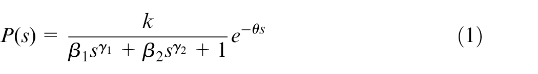
The proposed scheme is developed considering the non-integer (fractional) order plant with a transfer function.

$$P(s)=\frac{k}{{\beta }_1{s}^{{\gamma }_1}+{\beta }_2{s}^{{\gamma }_2}+1}{e}^{-\theta s}$$

(1)

where $k$ , ${\beta }_{1,2}>0$ , and ${\gamma }_{1,2}\in R^{+}$ are fractional-order. $P$ is fractional-second-order time-delay (FSOTD) system with ${\gamma }_1>{\gamma }_2$ . $k$ and $\theta$ are static gain and time delay, respectively. To note, ${\beta }_2=0$ becomes a fractional first-order time delay (FFOTD) model. Although the approach can regulate a controller for a general class of stable fractional systems, the validation part examines well-studied plant models from various classes.

Design target loop for FoRC

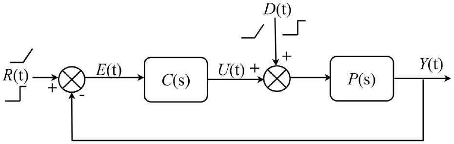
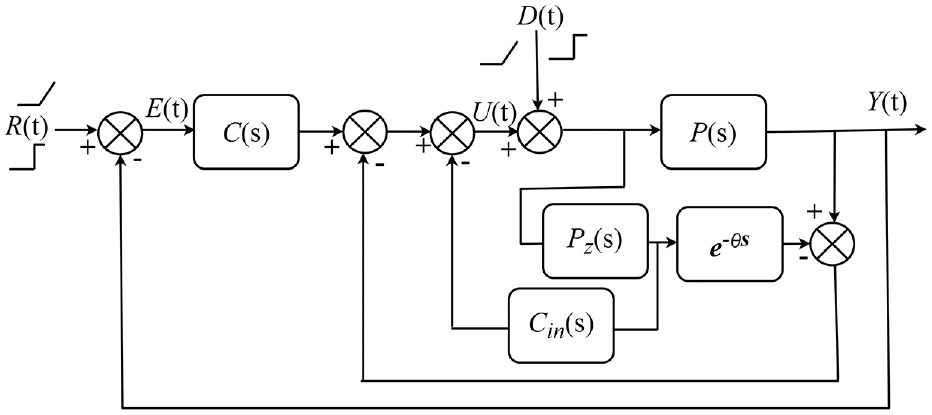
The challenge of efficiently handling higher-order references and disturbances persists despite the recent literature on controller design for fractional-order processes. Figure 1 depicts a typical closed-loop control architecture with $C(s)$ controlling the plant $P(s)$ . Also, variables $R(t)$ , $E(t)$ , $D(t)$ , $U(t)$ , and $Y(t)$ represent the reference, error, disturbance, control signal and output, respectively. The open loop transfer function (LTF) for the control structure in Figure 1 is represented as $L(s)=C(s)P(s)$ .

Figure 1.

Closed-loop control structure.

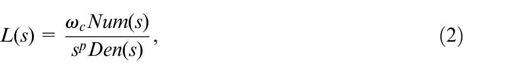
A technique known as target loop-based design is one in which an appropriate desired open loop is chosen first, and then a controller needs to be created to accomplish that. Conventional loop-shaping theories have the potential to affect the concept of target LTF. These theories stipulate that the target loop must include all of the non-invertible components of the process model. In a design of this kind, selecting the target loop $T(s)$ is of the utmost importance. The desired loop for a delayed open-loop stable system can be chosen as Bode’s ideal transfer function, ${\left(\frac{{\omega }_c}{s}\right)}^{\lambda }$ . ¹ Here ${\omega }_c$ represents the closed-loop bandwidth, and $\lambda \in R$ is the slope of the magnitude curve. Although this target loop can track step inputs and reject disturbances, it would fail to handle the ramp-type signals. We need more than one free integrator in the open-loop design to handle ramp-type servo tracking and disturbance rejection. Let us take LTF in general as below.

$$L(s)=\frac{{\omega }_{c}Num(s)}{s^{p}Den(s)},$$

(2)

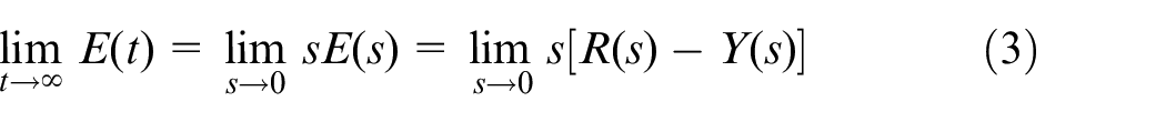
with $\mathrm{Num}(0)=\mathrm{Den}(0)=1$ and $p\in R$ . To achieve the tracking of ramp setpoints, it is necessary for $L(s)$ to have more than one free integrator. This requirement becomes apparent when analyzing the $E(t)$ over extended time intervals. Assuming the stability of the closed-loop system, we can employ the final value theorem of the Laplace transform for analysis.

$$\underset{t\to \infty }{lim}E(t)=\underset{s\to 0}{lim}\mathrm{sE}(s)=\underset{s\to 0}{lim}s[R(s)-Y(s)]$$

(3)

with the closed-loop $Y(s)/R(s)=L(s)/(1+L(s))$ . If the ramp signal $R(s)=A/s^2$ , we get

$$\underset{t\to \infty }{lim}E(t)=\underset{s\to 0}{lim}s\frac{R(s)}{1+L(s)}=\underset{s\to 0}{lim}s\frac{s^p\mathrm{Den}(s)R(s)}{s^p\mathrm{Den}(s)+\mathrm{Num}(s)}$$

(4)

$$=\left(\frac{0^{p-1}\mathrm{Den}(0)}{0^p\mathrm{Den}(0)+\mathrm{Num}(0)}\right)A.$$

(5)

The expression (5) becomes zero only when $p>1$ , which poses a challenge for integer-order controllers as each integrator introduces a phase loss. To stabilize the closed-loop system, it is essential to compensate for this phase loss by introducing minimum phase zeros to the controller. Considering the above observation, some modifications in the target loop selection are proposed below.

• The controller should have two integrators with minimum phase zero.

• The target loop can be parametrized as

$$T(s)=\frac{{\omega }_c(s+\sigma )}{s^2}{e}^{-\theta s}$$

(6)

In $T(s)$ , $\sigma$ is the trade-off between disturbance attenuation and step response overshoot and $\theta$ is the time delay of the original plant. The choice of ${\omega }_c$ can be made as ${\omega }_c=\alpha /\theta$ in the desired loop (6), with proper selection of tuning parameter $\alpha$ .

This target loop is required to select two parameters instead widely studied function $({\omega }_c/s{)}^{\lambda }$ for a given plant model.

• Remark 1. It is to note that literature ³¹ suggested to choose $\sigma$ between $(0.25-0.5){\omega }_c$ . However, there is a lack of justification or specific relation available.

Attempt to design the target loop with the proper selection procedure for $\sigma$ and $\alpha$ so that the closed-loop system achieves the desired performance and robustness. The following subsection provides the selection steps for both unknown parameters.

Explicit design for target loop parameters

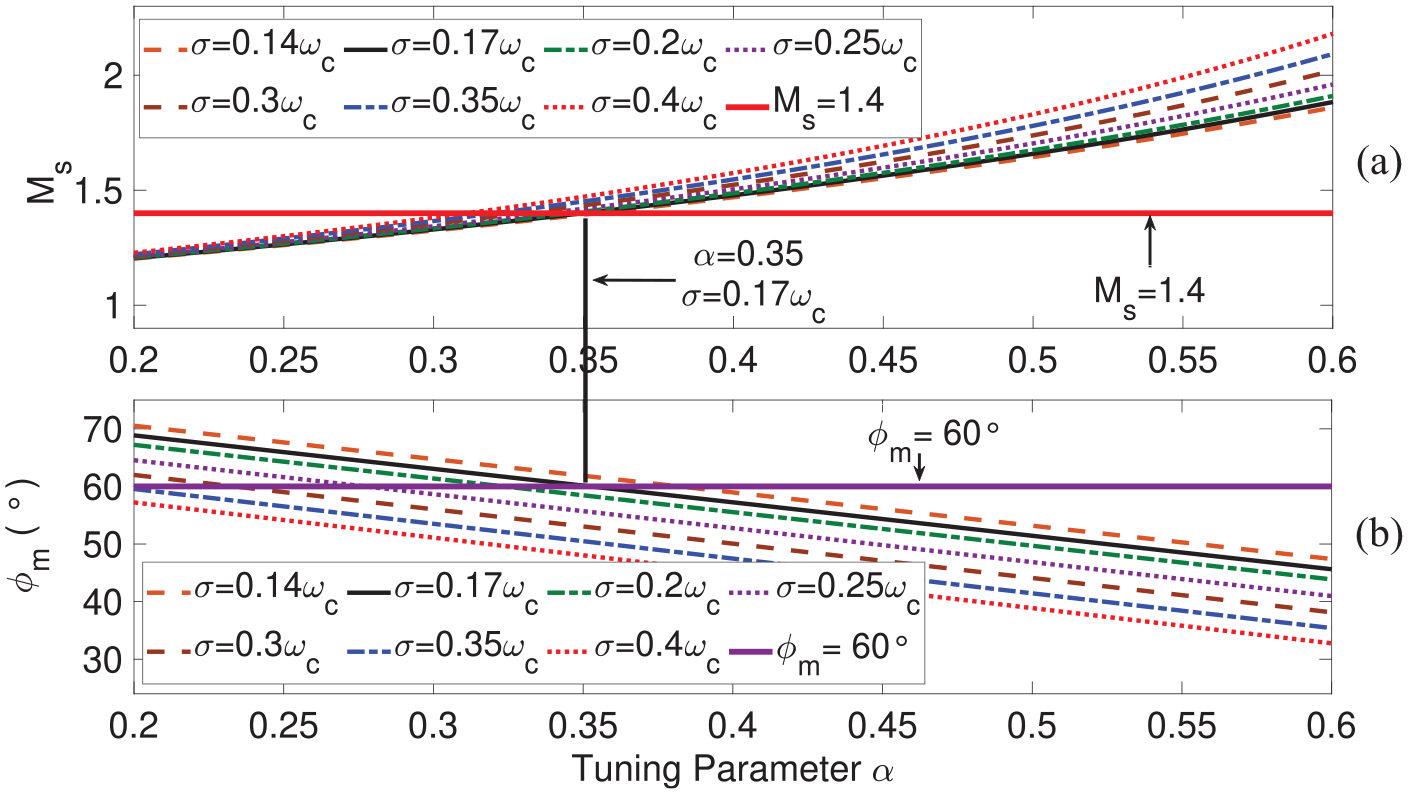
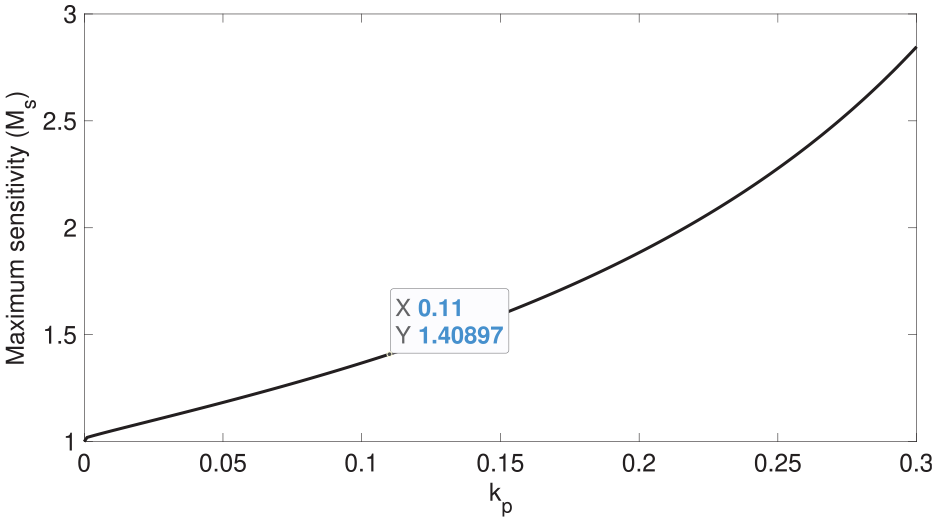
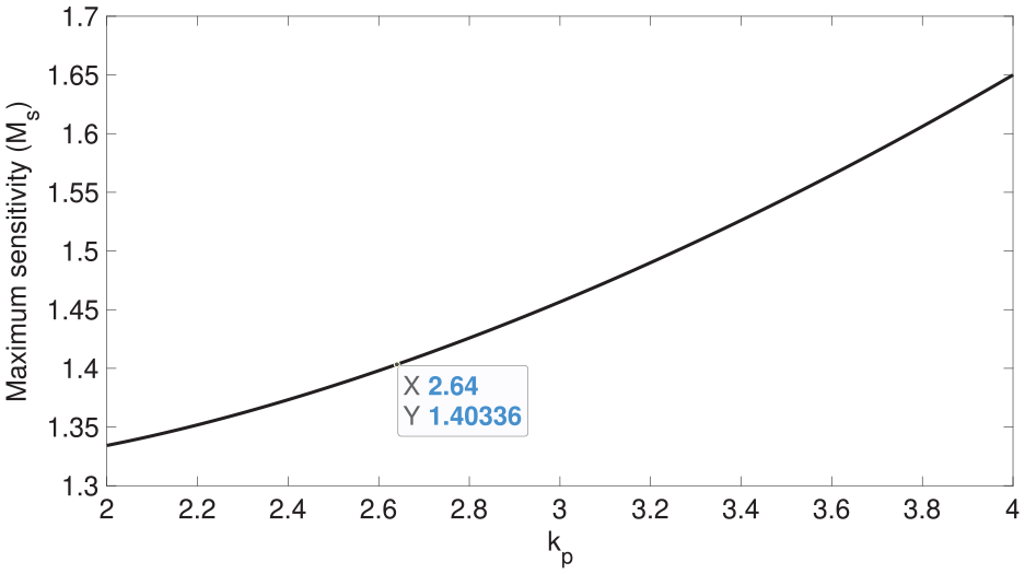
Target-loop parameters $\sigma$ and $\alpha$ have a close association with maximum sensitivity $(M_s)$ and phase margin $({\varphi }_m)$ . To achieve robust stability, $M_s$ of $T(s)$ should be in the range of $1.4-2.0$ and ${\varphi }_m$ fall within the stability range $(30°-60°)$ .^31,32 A higher degree of robustness is indicated by a higher value of ${\varphi }_m$ and a lower number of $M_s$ in the range. In contrast, a faster response with reduced robustness is suggested by a higher value of $M_s$ and a lower value of ${\varphi }_m$ . This work provides an analytical solution for unknown target loop values employing a graphical technique.

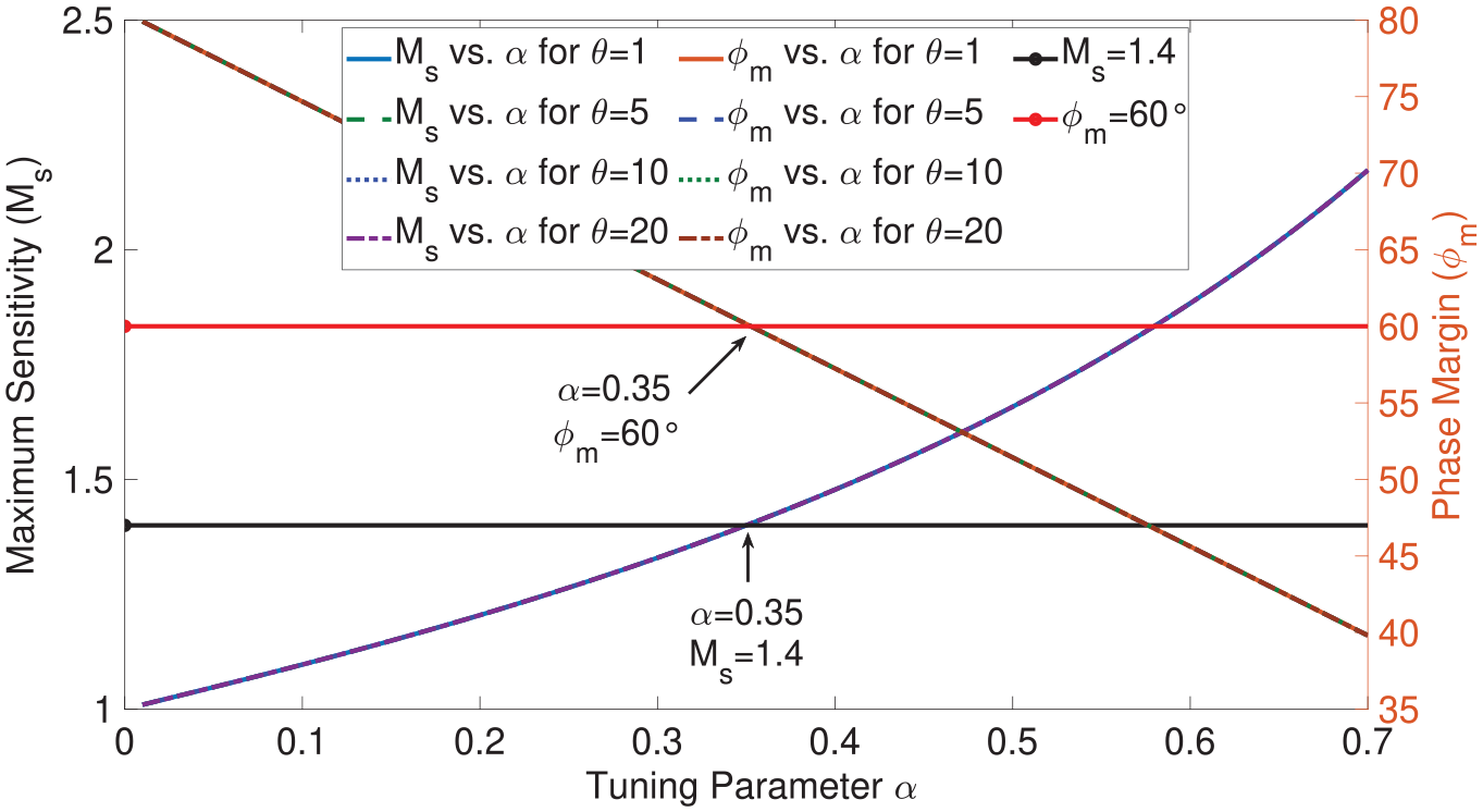
In order to strike a balance between robustness and performance in the closed-loop response, this study considers the values ${\varphi }_m=60°$ and $M_s=1.4$ . Due to the presence of two integrators in the designed LTF, the overshoot is possible. Thus, design criteria are selected to increase the robustness of the closed-loop system. Let us now assume ${\omega }_c=\alpha$ (i.e. $\theta =1$ ). The relation has been plotted as $\alpha$ versus $M_s$ and $\alpha$ versus ${\varphi }_m$ for different values of $\sigma$ . Interestingly, both the criteria for ${\varphi }_m=60°$ and $M_s=1.4$ are achievable at $\alpha =0.35$ and $\sigma =0.17{\omega }_c$ . As seen in Figure 2.

Figure 2.

Relation of $\alpha$ with $M_s$ and ${\varphi }_m$ for possible values of $\sigma$ .

• Remark 2. Design parameters ${\varphi }_m=60°$ and $M_s=1.4$ will always satisfy $\alpha =0.35$ and $\sigma =0.17{\omega }_c$ and confirm the independence of $\theta$ . When we plot the values of $M_s$ and ${\varphi }_m$ with $\sigma =0.17{\omega }_c$ and ${\omega }_c=\alpha /\theta$ in Figure 3 for varies $\theta =[1,5,10,20]$ , it has been found that $\alpha =0.35$ will always satisfy ${\varphi }_m=60°$ and $M_s=1.4$ . Therefore, an explicit expression can be written as,

$$\sigma =0.17{\omega }_c$$

(7)

$${\omega }_c=\frac{\alpha }{\theta }=\frac{0.35}{\theta }$$

(8)

Figure 3.

Selected value of $\alpha$ from $M_s=1.4$ and ${\varphi }_m={60}^{°}$ when $\sigma =0.17{\omega }_c$ .

Initially, the time delay is set to 1, making ${\omega }_c$ equal to $\alpha$ . Graphs are then plotted of $\alpha$ versus $M_s$ and $\alpha$ versus ${\varphi }_m$ for various values of $\sigma$ , as shown in Figure 2. From Figure 2, it can be observed that both criteria, ${\varphi }_m=60°$ and $M_s=1.4$ , are achieved at $\alpha =0.35$ and $\sigma =0.17{\omega }_c$ . Subsequently, graphs are plotted of $\alpha$ , $M_s$ , and ${\varphi }_m$ with $\sigma =0.17{\omega }_c$ for different values of time delay, such as $\theta =1,5,10,$ and $20$ , as shown in Figure 3. From Figure 3, it can be observed that both design parameters, ${\varphi }_m=60°$ and $M_s=1.4$ , are consistently met at $\alpha =0.35$ and $\sigma =0.17{\omega }_c$ , regardless of the value of $\theta$ .

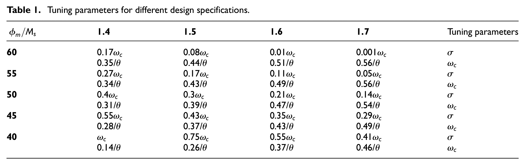
Similarly, a comprehensive compilation of explicit formulas and potential design specifications is presented in Table 1 to calculate the unknown parameters. Using these formulas, designers can determine the precise controller configurations that correspond to their designed specifications.

Table 1.

Tuning parameters for different design specifications.

${\varphi }_m/M_s$	1.4	1.5	1.6	1.7	Tuning parameters
60	0.17 ${\omega }_c$	0.08 ${\omega }_c$	0.01 ${\omega }_c$	0.001 ${\omega }_c$	$\sigma$
	0.35/ $\theta$	0.44/ $\theta$	0.51/ $\theta$	0.56/ $\theta$	${\omega }_c$
55	0.27 ${\omega }_c$	0.17 ${\omega }_c$	0.11 ${\omega }_c$	0.05 ${\omega }_c$	$\sigma$
	0.34/ $\theta$	0.43/ $\theta$	0.49/ $\theta$	0.56/ $\theta$	${\omega }_c$
50	0.4 ${\omega }_c$	0.3 ${\omega }_c$	0.21 ${\omega }_c$	0.14 ${\omega }_c$	$\sigma$
	0.31/ $\theta$	0.39/ $\theta$	0.47/ $\theta$	0.54/ $\theta$	${\omega }_c$
45	0.55 ${\omega }_c$	0.43 ${\omega }_c$	0.35 ${\omega }_c$	0.29 ${\omega }_c$	$\sigma$
	0.28/ $\theta$	0.37/ $\theta$	0.43/ $\theta$	0.49/ $\theta$	${\omega }_c$
40	${\omega }_c$	0.75 ${\omega }_c$	0.55 ${\omega }_c$	0.41 ${\omega }_c$	$\sigma$
	0.14/ $\theta$	0.26/ $\theta$	0.37/ $\theta$	0.46/ $\theta$	${\omega }_c$

Proposed controller design

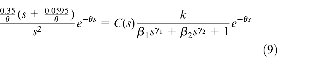
The explicit tuning expressions (7) and (8) can simplify the desired target loop function. Using the plant model (1) and target loop (6), once can write

$$\frac{\frac{0.35}{\theta }(s+\frac{0.0595}{\theta })}{s^2}{e}^{-\theta s}=C(s)\frac{k}{{\beta }_1{s}^{{\gamma }_1}+{\beta }_2{s}^{{\gamma }_2}+1}{e}^{-\theta s}$$

(9)

After rearranging, main FoRC $C(s)=C_1(s)C_2(s)$ can be developed where,

$$C_1(s)=(\frac{0.35}{k\theta }+\frac{0.02}{k{\theta }^2}\frac{1}{s})$$

(10)

and

$$C_2(s)=({\beta }_1{s}^{{\gamma }_1-1}+{\beta }_2{s}^{{\gamma }_2-1}+\frac{1}{s}).$$

(11)

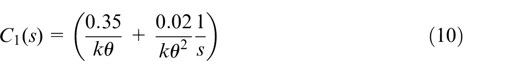
It is observed that $C_1$ is a simple PI and $C_2$ is a FoC. The controller gains can be calculated directly from the plant model’s parameters. Interestingly, the generalized controller $C_2$ exhibits various forms based on the model. For the FFOTD model ${\beta }_2=0$ and $C_2$ becomes,

$$C_2(s)=({\beta }_1{s}^{{\gamma }_1-1}+\frac{1}{s})$$

(12)

To note that when ${\gamma }_1<1$ , $C_2$ is defined as

$$C_2(s)=(\frac{{\beta }_1}{s^{1-{\gamma }_1}}+\frac{1}{s})$$

(13)

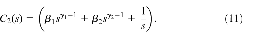
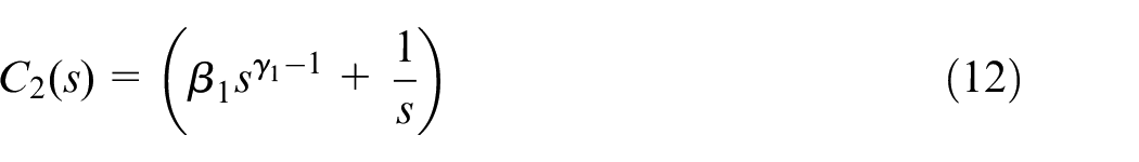
Let us take FSOTD model (1) and as per possible values of ${\gamma }_1$ and ${\gamma }_2$ , one can see the FoC as following. For ${\gamma }_2<1<{\gamma }_1$ , (11) can be written as:

$$C_2(s)=({\beta }_1{s}^{{\gamma }_1-1}+\frac{{\beta }_2}{s^{1-{\gamma }_2}}+\frac{1}{s})$$

(14)

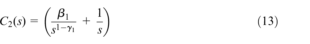
The same controller when $({\gamma }_1,{\gamma }_2)<1$ becomes

$$C_2(s)=(\frac{{\beta }_1}{s^{1-{\gamma }_1}}+\frac{{\beta }_2}{s^{1-{\gamma }_2}}+\frac{1}{s})$$

(15)

On other hand, integer controller $C_1$ remains unchanged regardless of the plant type or fractional-orders ${\gamma }_1$ and ${\gamma }_2$ .

Remark 3. Analyzing the robust stability of the closed-loop system or its family entails assessing the robust stability of its corresponding closed-loop characteristic polynomial(s). The assumed form of the continuous-time fractional-order uncertain polynomial is:

$$\begin{array}{c}\multicolumn{1}{c}{m(s,\mathbf{x})={\rho }_n(\mathbf{x})s^{z_n}+{\rho }_{n-1}(\mathbf{x})s^{z_{n-1}}+\dots +{\rho }_1(\mathbf{x})s^{z_1}}\\ \multicolumn{1}{c}{+{\rho }_0(\mathbf{x})s^{z_0}=\sum _{i=1}^n{\rho }_i(\mathbf{x})s^{z_i}}\end{array}$$

(16)

where $\mathbf{x}$ denotes the vector representing uncertainty, $z_n>\dots >z_0$ stand for real numbers and ${\rho }_i$ for $i=0,...,n$ represent coefficient functions.

Then the family of polynomials is defined as:

$$M=\{m(·,\mathbf{x}):\mathbf{x}\in X\}$$

(17)

where $X$ denotes the set that bounds the uncertainty. The family of polynomials (17) is robustly stable if and only if $m(s,\mathbf{x})$ is stable for all $\mathbf{x}\in X$ .

The value set for the family of polynomials (16) at the frequency $\omega \in R$ is defined as^33,34

$$m(j\omega ,X)=\{m(j\omega ,\mathbf{x}):\mathbf{x}\in X\}$$

(18)

The zero exclusion condition for ensuring the (Hurwitz) stability of the family of continuous-time polynomials (17) can be formulated according to.^33,34 Assume the polynomials in the family have an invariant degree, the uncertainty bounding set $X$ is pathwise connected, the coefficient functions ${\rho }_i$ for $i=0,...,n$ and there is at least one stable member $m(s,{\mathbf{x}}^0)$ . Then, the family $X$ is robustly stable if and only if the origin of the complex plane (zero point) is excluded from the set of values $m(j\omega ,X)$ for all frequencies $\omega \ge 0$ . In other words, $M$ is robustly stable if and only if

$$0\notin m(j\omega ,X)\forall \omega \ge 0$$

(19)

Remark 4. Stability of a fractional-order system can be determine by Matignon’s stability Theorem. Let us consider a fractional-order closed loop transfer function $T(s)=N(s)/D(s)$ . This system may be transformed from $s$ -plane to $\delta$ -plane. Now $T(s)$ is considered stable if and only if the following condition is satisfied^35–37:

$$|\arg (\delta )|>q\frac{\pi }{2},\forall {\delta }_i\in C,i^{\mathrm{th}}\mathrm{root}\mathrm{of}D(\delta )=0$$

(20)

where $\delta =s^q$ .

The stability of a fractional-order system can also be analyzed by examining its characteristic equation in the following form:

$$a_0{s}^{b_0}+a_1{s}^{b_1}+\dots +a_n{s}^{b_n}=\sum _{i=0}^n{a}_i{s}^{b_i}=0$$

(21)

For $b_i=\frac{h_i}{h}$ , transform the equation (21) into $\delta$ - plane:

$$\sum _{i=0}^n{a}_i{s}^{\frac{\mathrm{hi}}{h}}=\sum _{i=0}^n{a}_i{\delta }^{h_i}$$

(22)

where $\delta =s^{\frac{k_0}{m}}$ and $m$ represents the least common multiple of $h$ . For every value of $a_i$ , the roots of (22) is ${\varphi }_{\delta }=|\arg (\delta )|$ . Thus, the fractional-order system is stable if the following conditions are met:

$$\mathrm{For}\mathrm{stabile}\frac{\pi }{2m}<|\arg (\delta )|<\frac{\pi }{m}$$

(23)

$$\mathrm{For}\mathrm{oscillatory}\mathrm{stable}|\arg (\delta )|=\frac{\pi }{2m}$$

(24)

Case studies

Proton exchange membrane fuel cell

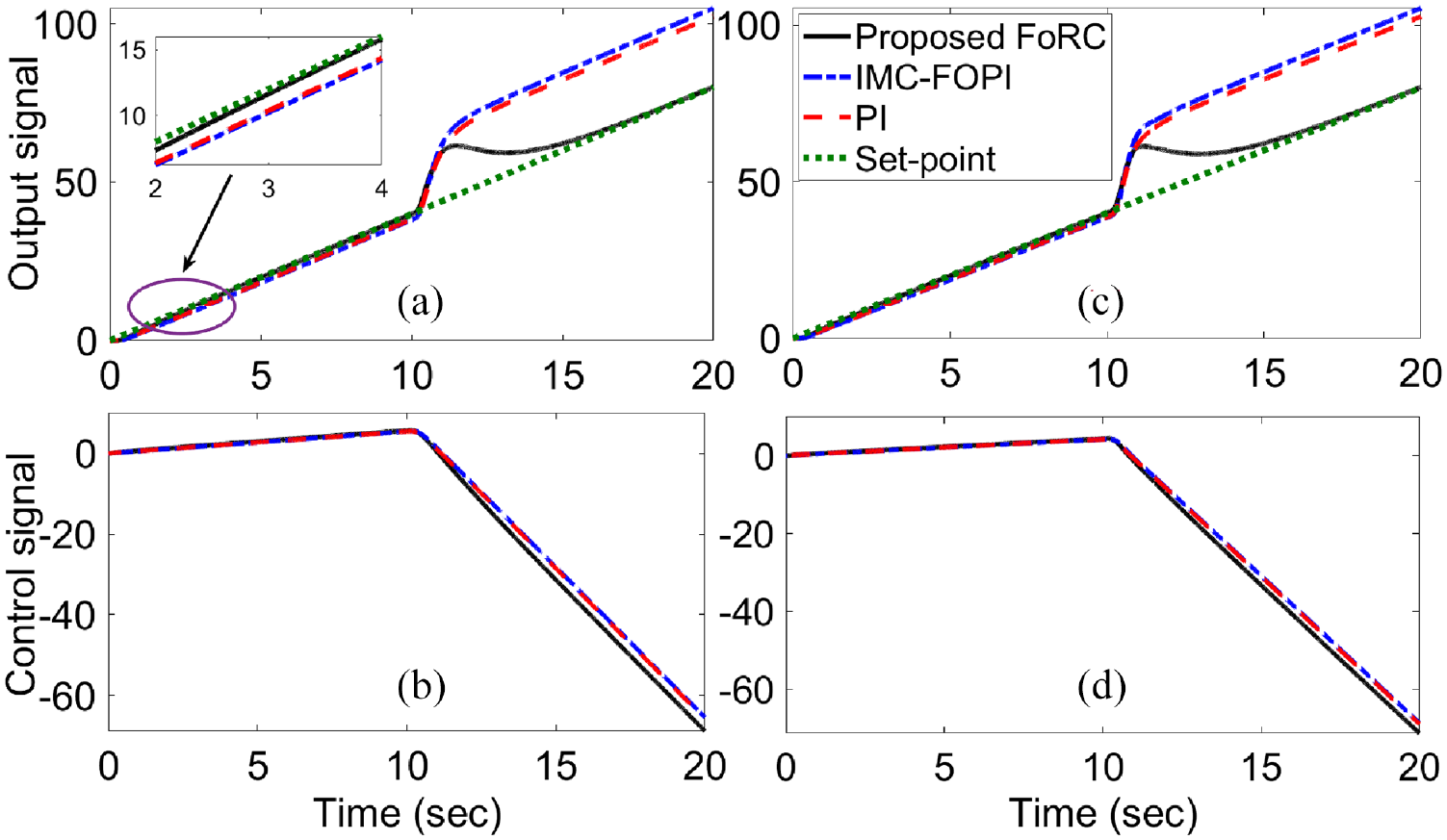
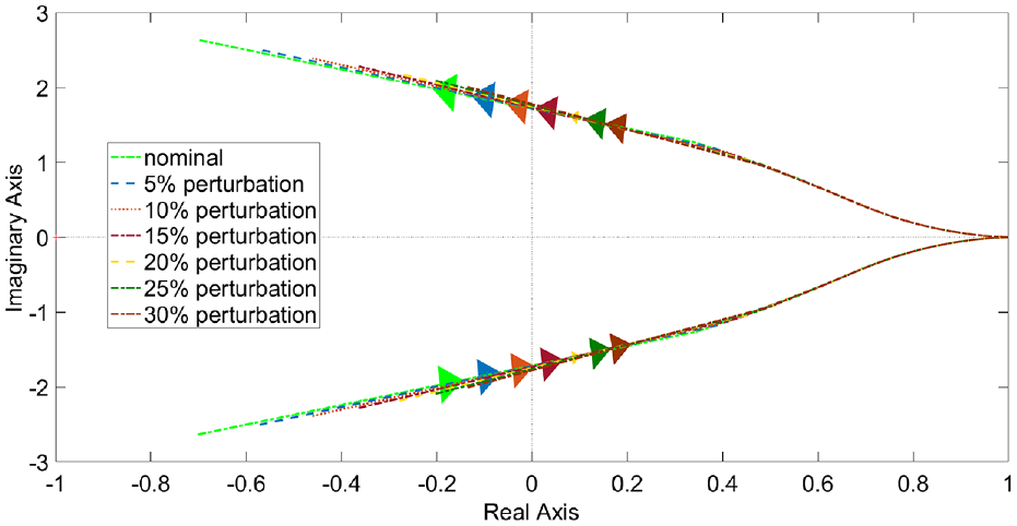
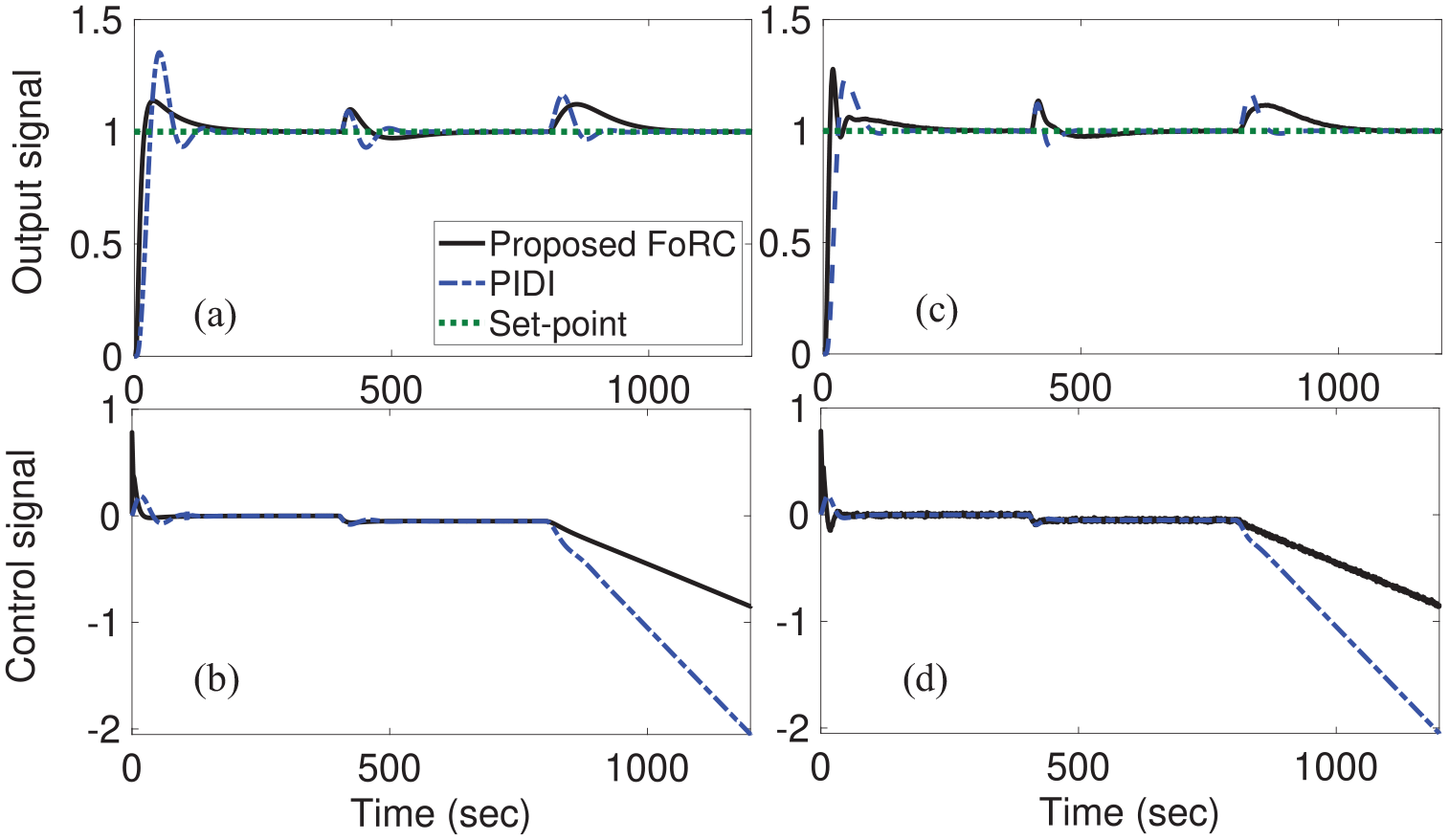
Let us consider a proton exchange membrane fuel cell system dominant with lag. ²⁸ It is represented by $P_1(s)=\frac{7.35}{0.368s^{1.02}+1}{e}^{-0.125s}$ . The authors in Reference ²⁸ suggested the PI controller $C(s)=(0.14+0.34/s)$ , while for the same plant, in Reference ²⁹ the IMC-FOPI controller was $(0.05+0.357/s)\left(\frac{0.0625s^{1.05}+s^{0.02}}{(0.0016s^2+0.0456s+0.445)}\right)$ .

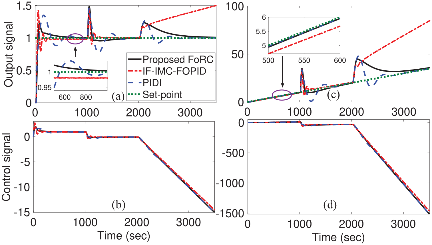
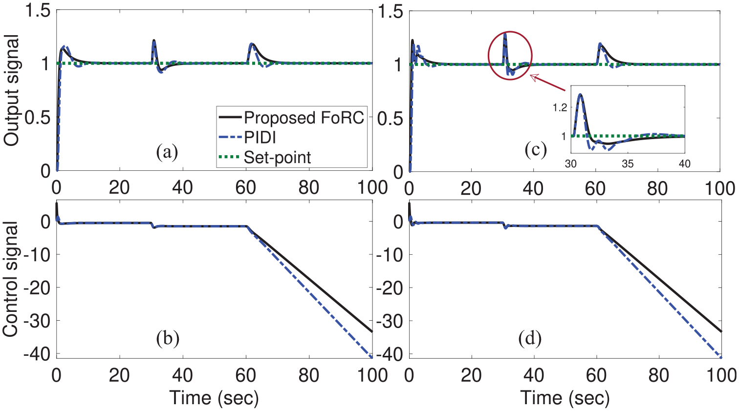
Now following the explicit design from Section “Proposed Controller Design,” the expressions provided in (10) and (12) are replaced by $C(s)=(0.381+0.183/s)(0.368s^{0.02}+1/s)$ . All controllers are verified for ramp set-point input. The output of the system is shown in Figure 4(a) and the corresponding control signals in Figure 4(b). The simulation was carried out with four ramp inputs with slopes of eight at 10 s. To verify the robustness with uncertainty in model parameters, we assume +30% changes in both $k$ and $\theta$ simultaneously. Figure 4(c) shows the outcomes and corresponding control signals are plotted in Figure 4(d). One can see that the proposed fractional ramp controller can track the ramp signal and also reject load disturbance of type ramp effectively. The designs^28,29 can not handle ramp signals.

Figure 4.

Ramp tracking $P_1$ : (a) Output (b) Control signal (c) Perturbed output (d) Perturbed control signal.

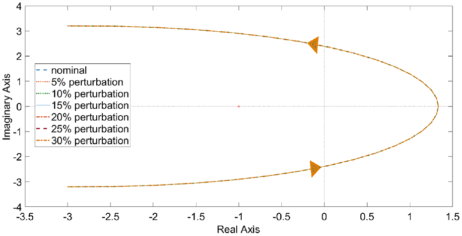
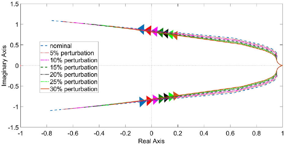
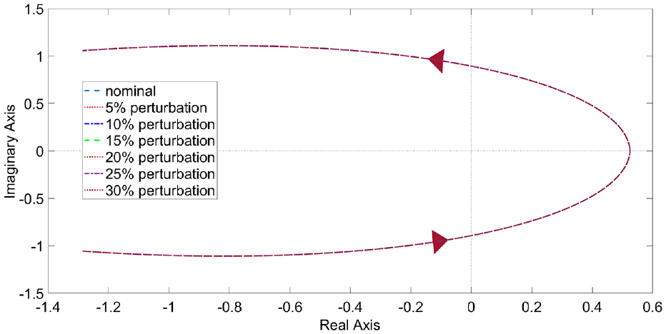
Additionally, to check robustness with an uncertainty bounding set ranging from 0% to 30% variations in both $k$ and $\theta$ , the family of closed-loop characteristic polynomials is defined as:

$$1+L(s)=1+P_1(s)C(s)=0$$

(25)

The value sets of polynomials (25) are plotted in Figure 5 for the frequency range from 0 to 1.5 with step 0.1. The family of (25) is identified as robustly stable, meeting the zero exclusion condition as discussed in Remark 3.

Figure 5.

Value sets of characteristic polynomials for $P_1(s)$ .

After transformation in the $\delta$ -plane, the roots of characteristic polynomial in (25) are obtained as $\delta =-3.7041\pm 2.0725i$ , $-0.5918$ and with these roots, the outcome of (23) is $-1.57<2.6315<3.14$ . Hence, it shows that the system is stable.

Bio-reactor

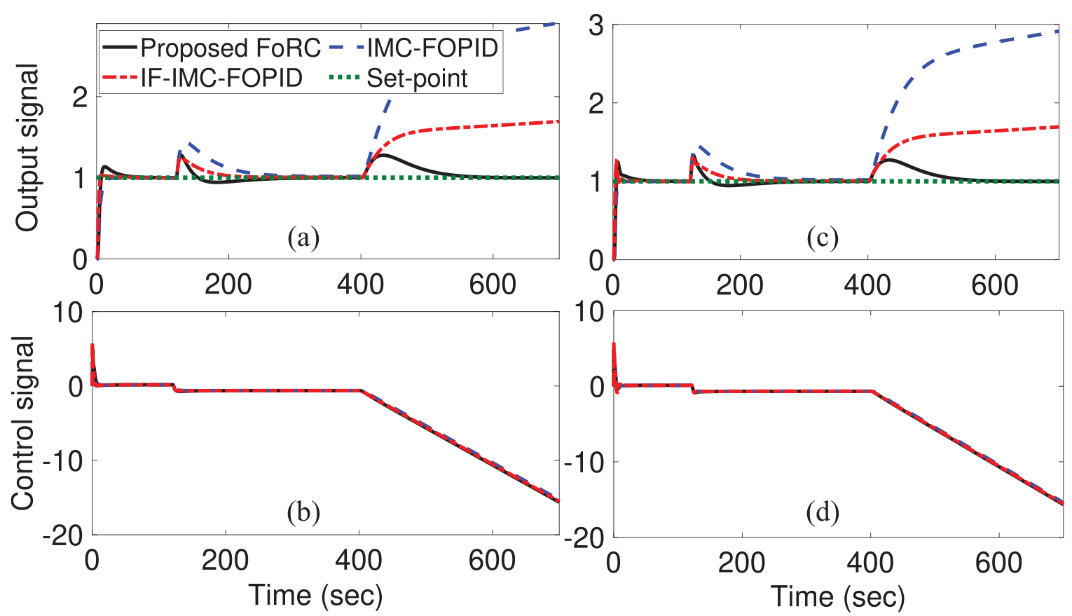
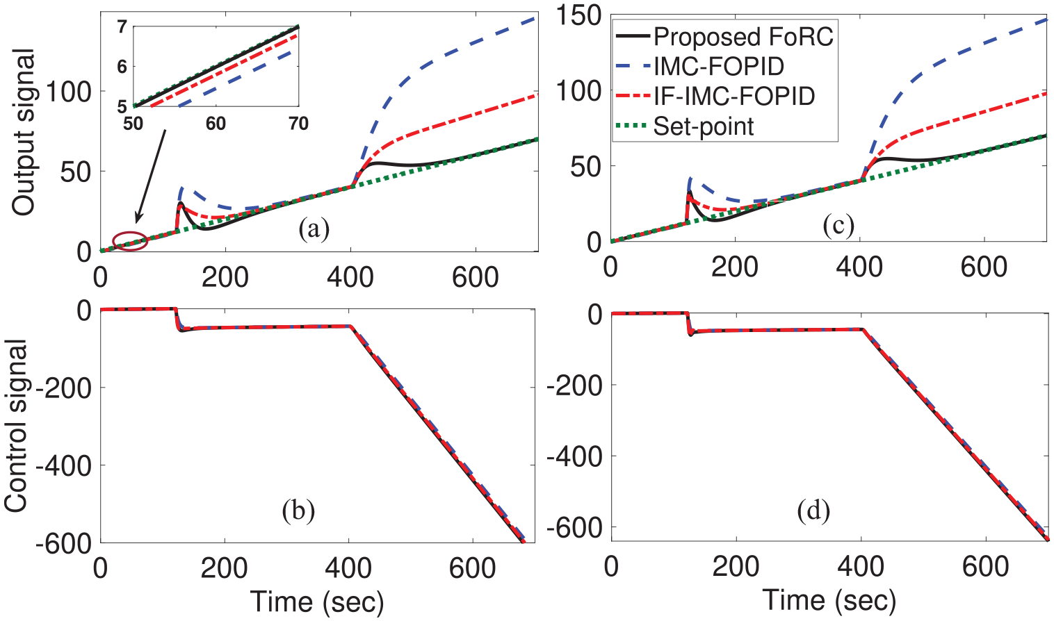
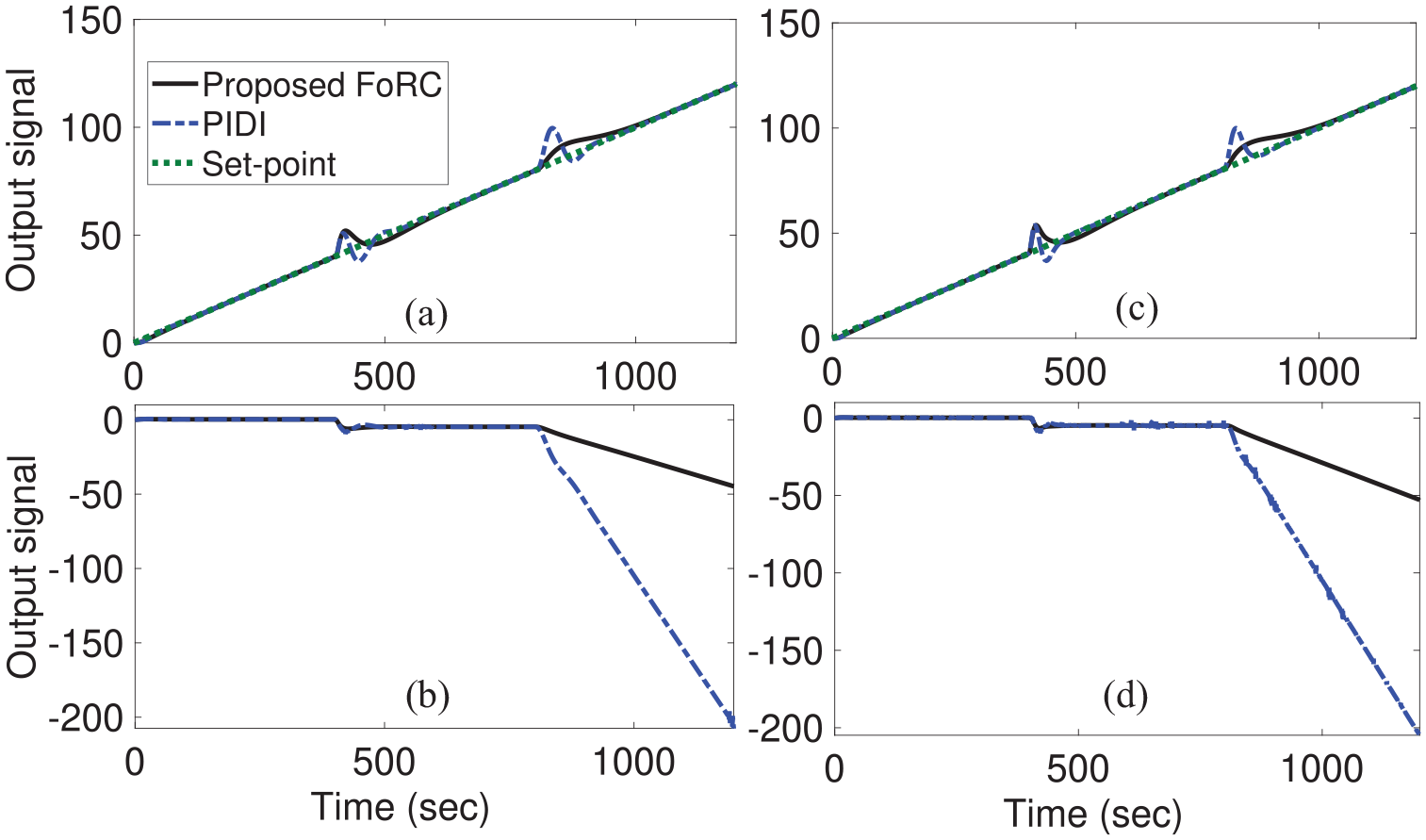
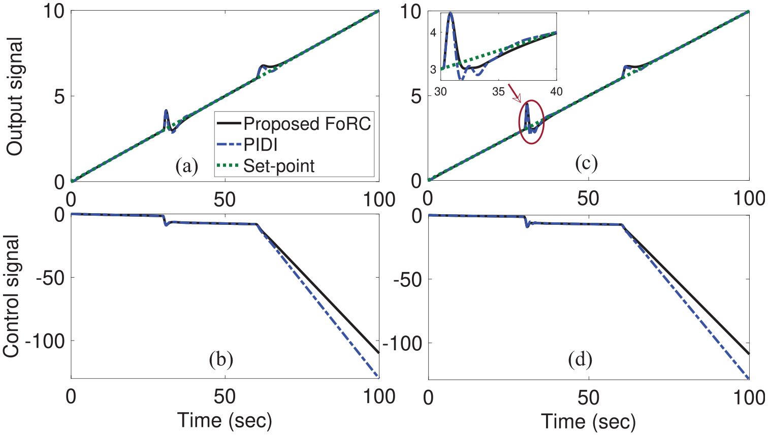
Let us consider a bioreactor model from^29,30 as $P_2(s)=\frac{5.8}{50.3s^{1.12}+7.8s^{0.95}+1}{e}^{-1.23s}$ . Indirect fractional IMC-FOPID (IF-IMC-FOPID) was suggested ³⁰ as

$C(s)=0.6217(1+\frac{0.1794}{s^{0.95}}+6.0722s^{0.17})\left(\frac{1}{1.23s^{0.95}}\right)$ . For the same plant, the higher-order IMC-FOPID structure by ²⁹ was $C(s)=1.345(1+\frac{0.128}{s^{0.95}}+6.45s^{0.17})$ $\left(\frac{1+0.615s}{s^{0.05}(1.505s^2+4.372s+5.359)}\right)$ . Following the proposed FoRC in Section 4, the parameters were calculated directly using (10) and (14). Our method obtains the FoRC as $C(s)=(0.049+0.0024/s)(50.3s^{0.12}+7.8/s^{0.05}+1/s)$ .

The outputs are compared with^29,30 for the input type step and ramp signals. The respective plots are seen from Figures 6(a) and 7(a) and the corresponding control signals are also given in Figures 6(b) and 7(b), respectively. For Figure 6(a), simulation was performed with unit step input at $t=0$ sec, step disturbance of magnitude $+0.8$ at $t=120$ sec and ramp disturbance with slope 0.05 at 400 s.

Figure 6.

Step tracking $P_2$ : (a) Output (b) Control signal (c) Perturbed output (d) Perturbed control signal.

Figure 7.

Ramp tracking $P_2$ : (a) Output (b) Control signal (c) Perturbed output (d) Perturbed control signal.

The output indicated better results for the new FoRC. More importantly, Figure 7(a) shows the ramp tracking, having 0.1 slopped at $t=0$ sec. Also, assuming a step disturbance of magnitude ±50 at $t=120$  s and a ramp disturbance with slope two at 400 s. Again, the proposed method outperformed the others. Further, to check the effectiveness of uncertainties, a study conducted with +30% changes in both process gain and delay simultaneously. The results for step and ramp signals are plotted in Figures 6(c) and 7(c). Note that the designs from References^29,30 can only handle step setpoints. These results show that the proposed FoRC can effectively track and reject step and ramp signals together.

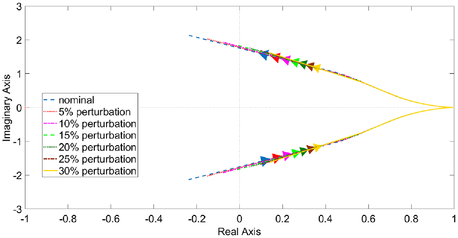
In addition, the robustness is checked with an uncertainty bounding set ranging from 0% to 30% variations in both $k$ and $\theta$ , the family of closed-loop characteristic polynomials is defined as $1+P_2(s)C(s)=0$ , and the value sets of polynomials are plotted in Figure 8. The family of polynomials is identified as robustly stable, meeting the zero exclusion condition as outlined in Remark 3.

Figure 8.

Value sets of characteristic polynomials for $P_2$ .

After transformation in the $\delta$ -plane, the roots of a characteristic polynomial for this case study are obtained as $\delta =-0.3764\pm 0.2106i$ , $-0.0601$ and with these roots, the outcome of (23) is $-1.57<2.6315<3.14$ . Hence, it shows that the system is stable.

Conical water tank system

Let us consider a large deadtime conical tank system studied in Reference. ³⁰ The plant model is given as $P_3(s)=\frac{1.0409}{7.6433s^{0.75373}+7.204s^{0.50732}+1}{e}^{-15.076s}$ .

The IF-IMC-FOPID in Reference ³⁰ was $C(s)=\frac{6.9209}{15.076s^{0.49268}}(1+\frac{0.1388}{s^{0.50732}}+1.061s^{0.2464})$ . Now following the design presented in Reference, ³¹ the PIDI controller for the same plant was calculated as $C(s)=(0.0279+\frac{0.0003}{s}+1.0459s)\frac{1}{s}$ . Now using (10) and (15), we have obtained $C(s)=(0.022+0.000084/s)(\frac{7.6433}{s^{0.24627}}+\frac{7.204}{s^{0.49268}}+\frac{1}{s})$ .

Performances are compared with step and ramp setpoints, with +30% perturbations in $k$ and $\theta$ . Figure 9(a) shows a unit step reference at $t=0$  s, a step disturbance of magnitude ±1 at $t=1000$ sec and a ramp disturbance with slope 0.01 at 2000 s. Figure 9(c) shows 0.01 slopped ramp input at $t=0$  s a step disturbance of magnitude +50 at $t=1000$  s and ramp disturbance with slope one at 2000 s. Corresponding control signals are plotted in Figure 9(b) and (d), respectively. Again, it is proven from the comparative results that the proposed controller can handle both situations better with fewer tuning parameters.

Figure 9.

Perturbed $P_3$ : (a) Step tracking output. (b) Control signal. (c) Ramp tracking output. (d) Control signal.

Further, the robustness is checked with an uncertainty bounding set ranging from 0% to 30% variations in both $k$ and $\theta$ , the family of closed-loop characteristic polynomials is defined as $1+P_3(s)C(s)=0$ , and the value sets of the polynomials are plotted in Figure 10. The family of polynomials is identified as robustly stable, meeting the zero exclusion condition as outlined in Remark 3.

Figure 10.

Value sets of characteristic polynomials for $P_3$ .

After transformation in the $\delta$ -plane, the closed-loop roots for this particular case study are obtained as $\delta =-0.0307\pm 0.0172i$ , $-0.0049$ and with these roots, the outcome of (23) is $-1.57<2.6315<3.14$ . Hence, it shows that the system is stable.

Extension of the proposed FoRC method to a broad class of systems

The explicit approach can be extended to a broad class of plants. In order to handle other model types, the control structure in Figure 1 has been modified as shown in Figure 11. In this figure, $C_{\mathrm{in}}(s)$ is a proportional-derivative (PD) controller in the inner loop to stabilize the plant and $P_z(s)$ is the delay-free part of the process.

Figure 11.

Modified closed-loop control structure.

In this modification, both controllers are designed independently. Firstly, the $C_{\mathrm{in}}(s)$ controller is tuned using the maximum sensitivity criterion. Following this, $C(s)$ is designed using the same target loop approach as explained previsouly.

Design of $C_{\mathrm{in}}(s)$ for fractional integrating processes

Let us consider a fractional integrating process as:

$$P(s)=\frac{k}{s^{{\gamma }_1}}{e}^{-\theta s}$$

(26)

and inner loop controller $C_{\mathrm{in}}(s)$ taken as a PD controller. So, one can write

$$C_{\mathrm{in}}(s)=k_p(1+{\tau }_{d}s)$$

(27)

Now, from Figure 11, the closed loop transfer function of the inner loop can be written as:

$$P_{\mathrm{in}}(s)=\frac{1}{1+P_z(s)C_{\mathrm{in}}(s)}P(s)$$

(28)

Now consider ${\tau }_d$ as $\frac{\theta }{2}$ and using (26) and (27), equation (28) can be simplified as:

$$P_{\mathrm{in}}(s)=\frac{k_{\mathrm{in}}}{{\beta }_1{s}^{{\gamma }_1}+{\beta }_{2}s+1}{e}^{\theta s}$$

(29)

where $k_{\mathrm{in}}=k/k{k}_p$ , ${\beta }_1=1/k{k}_p$ and ${\beta }_2=\theta /2$ with ${\gamma }_2=1$ .

Design of $C_{\mathrm{in}}(s)$ for fractional unstable processes

Let us consider a fractional unstable process as:

$$P(s)=\frac{k}{\beta s^{{\gamma }_1}-1}{e}^{-\theta s}$$

(30)

By employing equations (27) and (28), along with (30), the inner closed-loop transfer function can be represented as:

$$P_{\mathrm{in}}(s)=\frac{k_{\mathrm{in}}}{{\beta }_1{s}^{{\gamma }_1}+{\beta }_{2}s+1}{e}^{\theta s}$$

(31)

where $k_{\mathrm{in}}=k/k{k}_p-1$ , ${\beta }_1=\beta /k{k}_p-1$ and ${\beta }_2=k{k}_p\theta /2(k{k}_p-1)$ with ${\gamma }_2=1$ .

The value of single tuning parameter $k_p$ will be determined based on the constraints of $M_s$ . So, to design the inner loop controller, maximum sensitivity can be represented as:

$$M_s=\Vert \frac{1}{1+P(s)C_{\mathrm{in}}(s)}{\Vert }_{\infty }$$

(32)

To obtain the appropriate value of $k_p$ for both integrating and unstable processes, $M_s=1.4$ is selected.

Now, with zero external disturbances and no discrepancy between the original plant and the plant model, the open-loop transfer function from Figure 11 and (28) can be expressed as:

$$L(s)=P_{\mathrm{in}}(s)C(s)$$

(33)

Next, according to the design procedure provided in Section “Proposed Controller Design,” the outer-loop controller $C(s)=C_1(s)C_2(s)$ is designed for the complete inner-loop transfer function $P_{\mathrm{in}}(s)$ and can be expressed as:

$$C_1(s)=(\frac{0.35}{k_{\mathrm{in}}\theta }+\frac{0.02}{k_{\mathrm{in}}{\theta }^2}\frac{1}{s})$$

(34)

and

$$C_2(s)=({\beta }_2+\frac{1}{s}+{\beta }_1{s}^{{\gamma }_1-1}).$$

(35)

To evaluate the applicability of the proposed method in a wide range of systems, some additional case studies have been conducted as follows. The results are presented in the subsequent subsections below.

Integrating process

Let us consider a fractional integrating model as $P_4(s)=\frac{0.2}{s^{1.11}}{e}^{-4s}$ . Following the design presented in Reference, ³¹ the inner loop PD controller for the same plant was calculated as $C_{\mathrm{PD}}(s)=0.344(1+1.9315s)$ and the outer loop PIDI controller was given as $C_{\mathrm{PIDI}}(s)=(0.0299+\frac{0.0011}{s}+0.1593)\frac{1}{s}$ . For the proposed method, the inner loop controller parameters are obtained as $k_p=0.11$ from Figure 12 and ${\tau }_d=2$ . From (34) and (35), the outer loop controller $\mathrm{FoRC}$ is calculated as $C(s)=(0.0098+0.00014/s)$ $(2+\frac{1}{s}+44.6429s^{0.11})$ .

Figure 12.

$M_s$ plot for integrating process to choose $k_p$ .

The outputs are compared with Reference ³¹ for the inputs of the step and ramp signals. The respective plots are seen from Figures 13 (a) and 14 (a) and the corresponding control signals are also given in Figures 13(b) and 14(b), respectively. For Figure 13(a), simulation was performed with unit step input at $t=0$  s, step disturbance of magnitude $+0.05$ at $t=400$  s and ramp disturbance with slope 0.005 at 800 s. The output indicated better results for the new FoRC. Figure 14(a) shows the ramp tracking, which has $0.1$ slopped at $t=0$  s. Also, assuming a step disturbance of magnitude $+5$ at $t=400$  s and a ramp disturbance with slope 0.5 at 800 s. In the same way, the proposed method outperformed the others. In addition, to check the effectiveness of uncertainties, a study was conducted with +30% changes in both the gain and delay of the process simultaneously. The results for both the step and ramp signals are plotted in Figures 13(c) and 14(c). It is clear from these results that the proposed FoRC exhibits superior performance in terms of both servo and regulatory responses in the case of step signals while maintaining competitive performance in the presence of ramp signals.

Figure 13.

Step tracking $P_4$ : (a) Output. (b) Control signal. (c) Perturbed output. (d) Perturbed control signal.

Figure 14.

Ramp tracking $P_4$ : (a) Output. (b) Control signal. (c) Perturbed output. (d) Perturbed control signal.

Further, the robustness is checked with an uncertainty bounding set ranging from 0% to 30% variations in both $k$ and $\theta$ , the family of closed-loop characteristic polynomials is defined as $1+P_4(s)C(s)=0$ , and the value sets of polynomials are plotted in Figure 15. The family of polynomials deemed robustly stable due to its fulfillment of the zero exclusion condition, as noted in Remark 3.

Figure 15.

Value sets of characteristic polynomials for $P_4$ .

After transformation in the $\delta$ -plane, the closed-loop roots for this particular case study are obtained as $\delta =-0.1158\pm 0.0.0648i$ , $-0.0185$ and with these roots, the outcome of (23) is $-1.57<2.6315<3.14$ . Hence, it shows that the system is stable.

Unstable process

Let us consider a fractional unstable process studied in Reference. ³⁸ The plant model is given as $P_5(s)=\frac{2}{2s^{1.2}-1}{e}^{-0.2s}$ . Following the design presented in Reference, ³¹ the inner loop PD controller for the same plant was calculated as $C_{\mathrm{PD}}(s)=2.64(1+0.1s)$ and the outer loop PIDI controller was given as $C_{\mathrm{PIDI}}(s)=(3.9996+\frac{2.8741}{s}+3.2325s)\frac{1}{s}$ . For the proposed method, the inner loop controller parameters are obtained as $k_p=2.64$ from Figure 16 and ${\tau }_d=0.1$ . From (34) and (35), the outer loop controller FoRC is calculated as $C(s)=(3.75+1.124/s)(0.124+\frac{1}{s}+0.467s^{0.2})$ .

Figure 16.

$M_s$ plot for unstable process to choose $k_p$ .

The outputs are compared with Reference ³¹ for the inputs of the step and ramp signals. The respective plots are shown in Figures 17(a) and 18(a) and the corresponding control signals are also given in Figures 17(b) and 18(b), respectively. For Figure 17(a), simulation was performed with unit step input at $t=0$  s, step disturbance of magnitude $+0.05$ at $t=400$  s and ramp disturbance with slope 0.005 at 800 s. The output indicated better results for the new FoRC. Figure 18(a) shows the ramp tracking, which has 0.1 slopped at $t=0$  s. Also, assuming a step disturbance of magnitude $+5$ at $t=400$  s and a ramp disturbance with slope 0.5 at 800 s. In the same way, the proposed method outperformed the others. In addition, to check the effectiveness of uncertainties, a study was conducted with +30% changes in both the gain and delay of the process simultaneously. The results for both the step and ramp signals are plotted in Figures 17(c) and 18(c). It is clear from these results that the proposed FoRC exhibits superior performance in terms of both servo and regulatory responses in the case of step signals while maintaining competitive performance in the presence of ramp signals.

Figure 17.

Step tracking $P_5$ : (a) Output. (b) Control signal. (c) Perturbed output. (d) Perturbed control signal.

Figure 18.

Ramp tracking $P_5$ : (a) Output. (b) Control signal. (c) Perturbed output. (d) Perturbed control signal.

Further, the robustness is checked with an uncertainty bounding set ranging from 0% to 30% variations in both $k$ and $\theta$ , the family of closed-loop characteristic polynomials is defined as $1+P_5(s)C(s)=0$ , and the value sets of polynomials are plotted in Figure 19. The family of polynomials deemed robustly stable due to its fulfillment of the zero exclusion condition, as discussed in Remark 3.

Figure 19.

Value sets of characteristic polynomials for $P_5$ .

After transforming into the $\delta$ -plane, the closed-loop roots for this case study are $\delta =-2.3150\pm 1.2953i$ , $-0.0049$ and with these roots, the outcome of (23) is $-1.57<2.6315<3.14$ . Hence, the system is shown to be stable.

Robustness verification

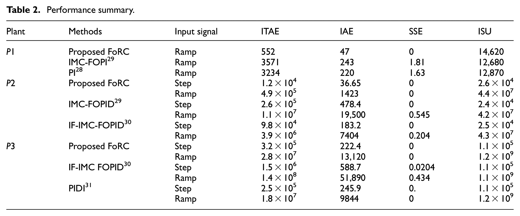
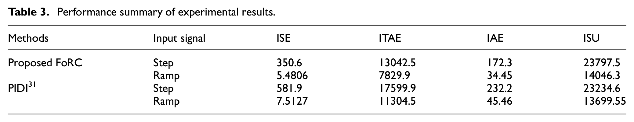
The quantitative values are calculated for comparisons such as ITAE, IAE, steady-state error (SSE) and the integral of the square of the control signal (ISU) in Table 2. It can be seen from the table that the FoRC demonstrates superior performance, particularly with ramp inputs, without any steady-state error.

Table 2.

Performance summary.

Plant	Methods	Input signal	ITAE	IAE	SSE	ISU
P1	Proposed FoRC	Ramp	552	47	0	14,620
	IMC-FOPI 29	Ramp	3571	243	1.81	12,680
	PI 28	Ramp	3234	220	1.63	12,870
P2	Proposed FoRC	Step	1.2 × 104	36.65	0	2.6 × 104
		Ramp	4.9 × 105	1423	0	4.4 × 107
	IMC-FOPID 29	Step	2.6 × 105	478.4	0	2.4 × 104
		Ramp	1.1 × 107	19,500	0.545	4.2 × 107
	IF-IMC-FOPID 30	Step	9.8 × 104	183.2	0	2.5 × 104
		Ramp	3.9 × 106	7404	0.204	4.3 × 107
P3	Proposed FoRC	Step	3.2 × 105	222.4	0	1.1 × 105
		Ramp	2.8 × 107	13,120	0	1.2 × 109
	IF-IMC FOPID 30	Step	1.5 × 106	588.7	0.0204	1.1 × 105
		Ramp	1.4 × 108	51,890	0.434	1.1 × 109
	PIDI 31	Step	2.5 × 105	245.9	0.	1.1 × 105
		Ramp	1.8 × 107	9844	0	1.2 × 109

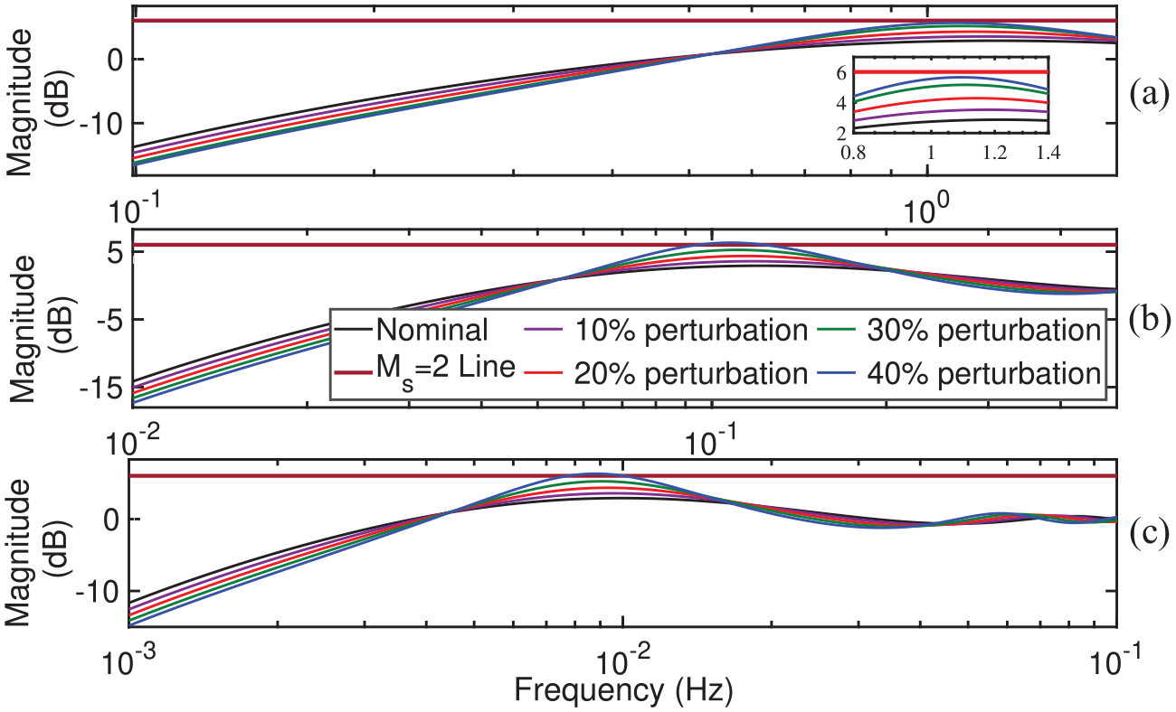
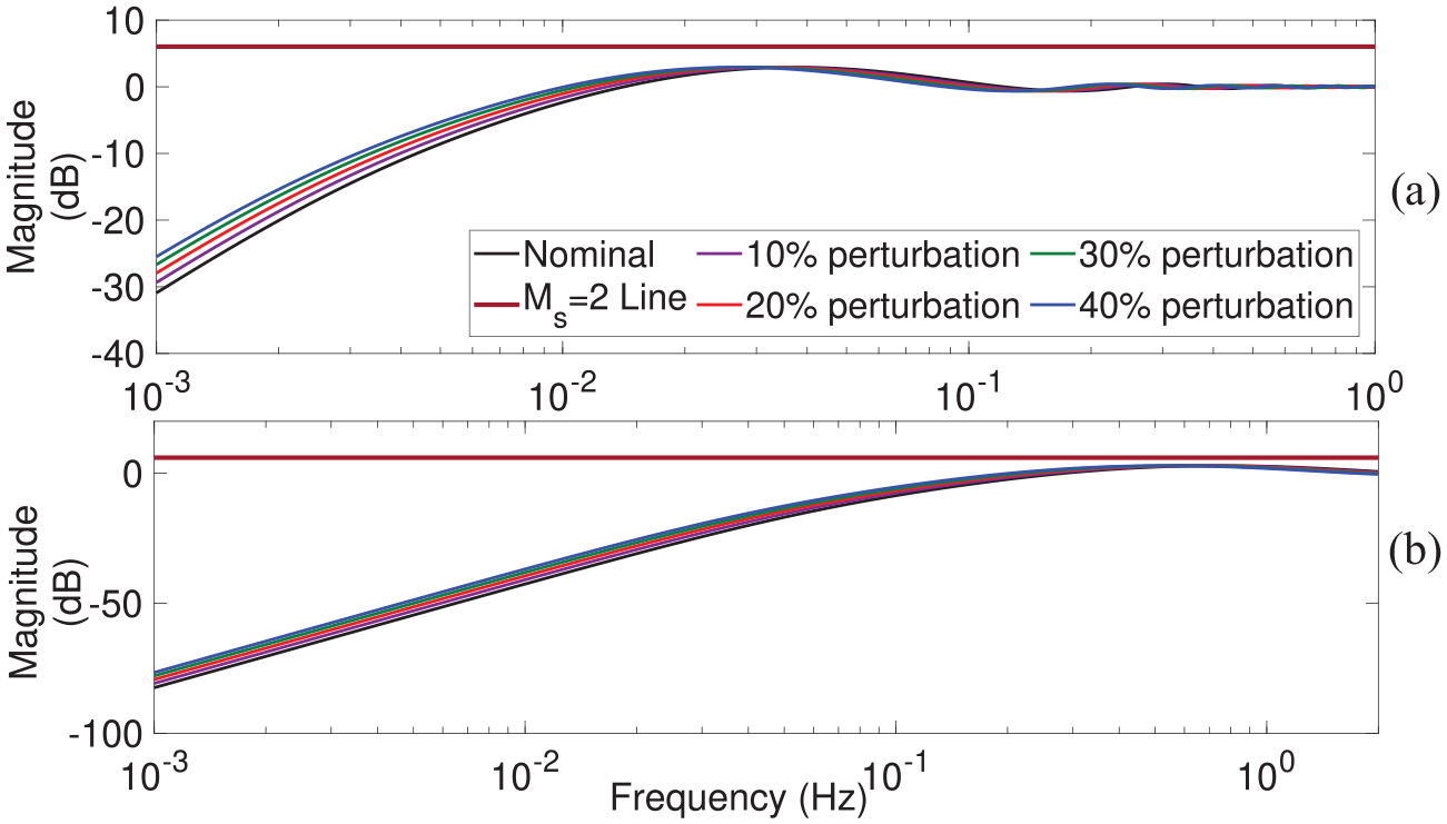
More importantly, the new controller was tested for parameter uncertainty. After changing the plant parameters and keeping the same controller setting, the maximum robustness index $M_s$ was achieved from the FoRC. The closed loop magnitude ensures the $M_s$ below 2 even after 40% changes in $k$ and $\theta$ together. Figures 20 and 21 show the perturbed results from all five examples. It is noted that the proposed design is capable of handling large perturbations.

Figure 20.

Robustness check for studied plants: (a) $P_1$ . (b) $P_2$ . (c) $P_3$ .

Figure 21.

Robustness check for extended studied plants: (a) $P_4$ . (b) $P_5$ .

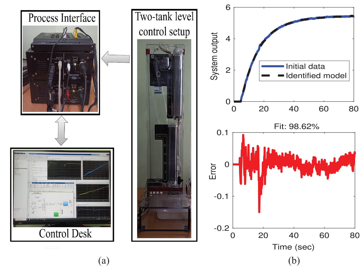
Experimental study

The novel FoRC was tested on a two-tank liquid level setup as seen from Figure 22(a). Here, water is supplied from a reservoir tank to a cascaded two-tank configuration through a water flow line. The control objective is considered to keep the level of tank 2 at its required set level by adjusting the input voltage to the pump.

Figure 22.

Liquid level control system. (a) Experimental setup. (b) Practical data and open-loop fractional-order model output.

A fixed voltage is applied to the pump in the setup and the water level in tank 2 is recorded. Using these measured output data, we have estimated a model of the practical setup. The Trust-Region Reflective Newton algorithm, with a 0.002 s sampling time, is employed in the system identification toolbox in MATLAB and the FOMCON toolbox to determine the parameters. The fractional order model of the actual plant, which achieves a fitness of 98.68% as shown in Figure 22(b), is identified as:

$$P(s)=\frac{1.1211}{11.16s^{1.056}+1}{e}^{-4.5s}$$

(36)

Implementing the proposed FoRC controller in two-tank liquid level setup is carried out using MATLAB/Simulink, employing the FOMCON toolbox. The effective implementation of the FoRC controller relies heavily on employing fractional-order integral and differential components. The Oustaloup approximation technique is one of the most commonly employed methods to derive fractional-order approximations. The FoRC controller with optimal parameters $({\omega }_b,{\omega }_h)=({10}^{-3},{10}^3)$ (frequency range) and $N=5$ (order of approximation) is used considering complexity and accuracy.

Following the proposed method and using explicit formulas from (10) and (12), we obtained $C(s)=(0.069+0.00093/s)(11.16s^{0.056}+1/s)$ . For the same plant, the PIDI controller using the latest method in Reference ³¹ was calculated as $C(s)=(0.0755+0.0023/s+0.9516s)\frac{1}{s}$ .

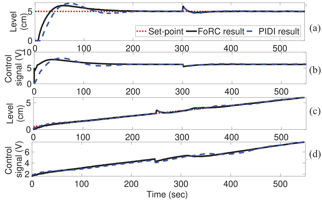
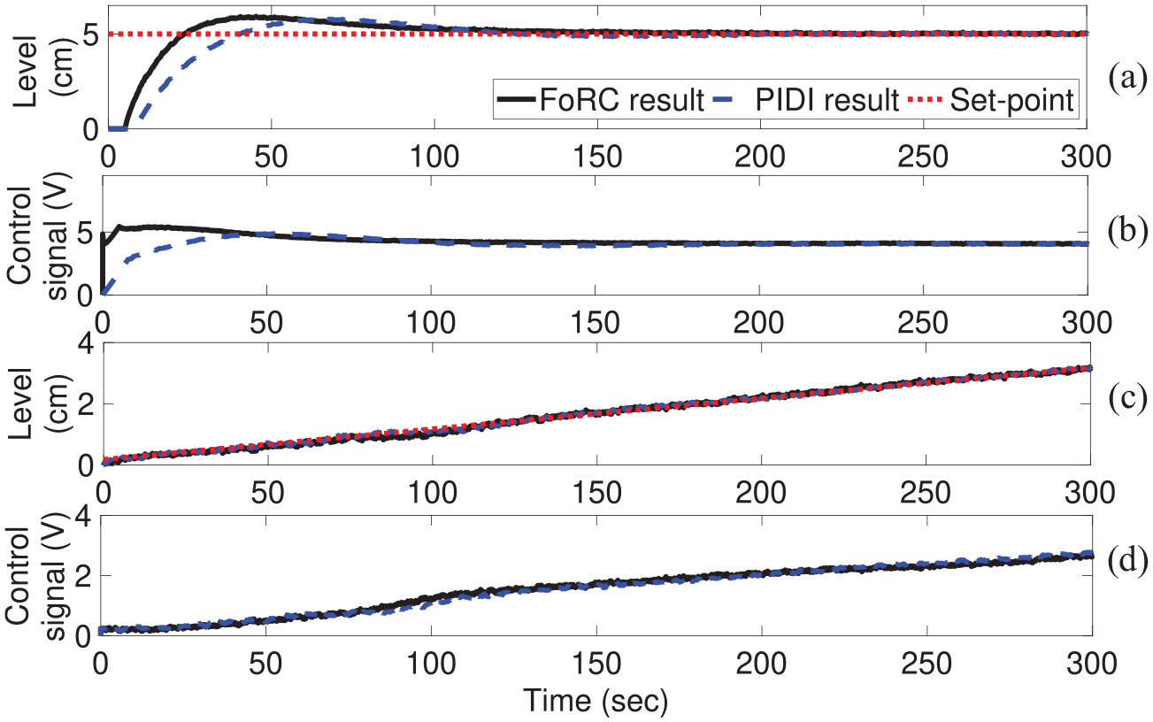
Firstly, we have checked the performance of the step tracking. The required water level was set at 5 cm, and to verify the regulatory result, a small amount of water was manually added as a disturbance in tank 2 at 300 s. The output result is seen from Figure 23(a) and corresponding control signal in Figure 23(b). More importantly, we have verified the performance with the ramp setpoint. The experiment was carried out with a 0.01 sloped ramp input with a manually added disturbance at 250 s. The ramp tracking results are seen from Figure 23(c) and (d). It is clear from the real-time tests that the proposed FoRC exhibits superior performance in terms of both servo and regulatory responses in the case of step signals while maintaining competitive performance in the presence of ramp signals.

Figure 23.

Experimental results: Step tracking: (a) Output. (b) Control. Ramp tracking: (c) Output. (d) Control.

Quantitative analysis of the experimental results

The quantitative values are calculated for comparisons like ISE, ITAE, IAE, ISU in Table 3. It can be seen from the table that the FoRC demonstrates superior performance in all cases.

Table 3.

Performance summary of experimental results.

Methods	Input signal	ISE	ITAE	IAE	ISU
Proposed FoRC	Step	350.6	13042.5	172.3	23797.5
	Ramp	5.4806	7829.9	34.45	14046.3
PIDI 31	Step	581.9	17599.9	232.2	23234.6
	Ramp	7.5127	11304.5	45.46	13699.55

Furthermore, to evaluate the efficiency of the proposed controller under the influence of a step disturbance as well as modeling variations, an experiment is conducted with the disturbance valve kept open. Keeping the same initial controller values, the results are obtained again. As seen in Figure 24, the proposed approach provided consistent performance even when the plant varied and step disturbances were presented.

Figure 24.

Experimental results with modeling variations and step disturbance: Step tracking: (a) Output. (b) Control. Ramp tracking: (c) Output. (d) Control.

Conclusions

This paper presented a target loop-based fractional-order control technique for fractional-order plant models. Unlike the most prevalent techniques on PID and FOPID, a new FoRC can handle changing ramp signals. The plant model and the desired robustness generated the explicit relation for the tuning of the parameters. When the design was validated using industrial processes and compared to other high-order fractional controllers, the new FoRC exceeded expectations. It can be seen from the quantitative analysis that the FoRC demonstrates superior performance, particularly with ramp inputs, without any steady-state error. The proposed design can also handle large perturbations in the parameters of the plant model, up to 40% simultaneously in $k$ and $\theta$ . Experimentation has demonstrated that the design steps are straightforward and realizable in real time. In addition, the detailed experimental analysis proves the value of the tuning approach. The authors are of the opinion that the method will contribute significantly to industrial fractional-order control. Extending the application of FoRC to more complex industrial systems, including multi-input multi-output systems, could be considered as the future scope of the work.