
Abstract
The switched inertance hydraulic converter is a sub-domain of digital hydraulics which relies on digital switching to adjust pressure or flow instead of the dissipation of power by throttling, providing an energy-efficient alternative to conventional proportional or servo valve-controlled systems. The high-speed switching valve is a key component to realise the digital switching and its switching characteristics has significant effects on the performance of switched inertance hydraulic converters. In this article, the switching characteristics of a high-speed rotary valve are investigated. The switching orifice area of the valve is calculated based on the movement of the valve components with a consideration of the design of the valve body and leakage. This is validated using the computational fluid dynamics model and in experiments. The valve is theoretically modelled considering the switching orifice, leakage, transition throttling and compressibility effect, and the results are validated by computational fluid dynamics and experimental tests. The valve is able to deliver a flow rate of 40 L/min at a pressure drop of 10 bar and switch at the maximum frequency of 317 Hz, with a switching transition time of about 1 ms, which shows promising performance for the use in digital hydraulics. The theoretical and computational fluid dynamics models can assist the design and optimisation of digital high-speed rotary valves, which can be very useful for understanding, analysing and optimising the characteristics and performance of switched inertance hydraulic converters in digital hydraulics.
Keywords
Introduction
The switched inertance hydraulic converter (SIHC) concept is a sub-domain of digital hydraulics which provides a novel alternative to conventional proportional or servo valve-controlled systems in fluid power. A typical SIHC consists of high-speed switching valves, inertance tubes and accumulators. 1 It can be configured in a variety of ways, such as a flow booster, 2 pressure booster, 3 bi-directional four-port converter and switching gyrator 4 for a wide range of hydraulic applications. Figure 1 shows the configuration of a flow booster that can deliver more flow than the supply flow. A 3/2-way high-speed switching valve is driven by a pulse width modulated (PWM) signal and switches alternately between the high-pressure (HP) supply port and low-pressure (LP) supply port. When the valve connects to the HP port, the high-velocity fluid passes from the HP port to the load; when the valve switches from the HP port to the LP port, the momentum of the fluid in the inertance tube draws flow from the LP port to the load despite the adverse pressure gradient. As long as the switching frequency of the valve is high, the ripple in delivery flow will be very small, and the average delivery flow rate can be significantly higher than the supply flow rate. The lower supply flow demand reduces power loss in comparison to using a throttling valve to control the flow to the load.
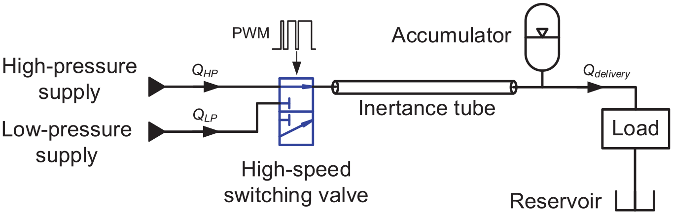
Schematic of a three-port flow booster. 5
A high-speed switching valve is the key component of an SIHC and its leakage, resistance and switching characteristics can significantly affect system efficiency. The switching valve should be able to operate with a high switching frequency, a low leakage, and deliver a high flow rate with a low pressure drop (low resistance). A variety of high-performance switching valves have been developed in the last 10 years, which were summarised in Yuan et al. 5 and categorised as rotary valves and linear valves, including spool valves and poppet valves. For spool valves, high flow rate with a low pressure drop can be achieved by increasing orifice area to reduce the valve resistance, such as 100 L/min at 5 bar in Manhartsgruber, 6 90 L/min at 5 bar in Winkler and Scheidl, 7 45 L/min at 5 bar in Winkler and Scheidl 8 and 50 L/min at 10 bar in Johnston et al., 9 but the switching frequency is typically limited to under 100 Hz at high flow rates due to the spool inertia. Poppet valves can achieve fast response (around 1 ms) and high flow rate by introducing multi-poppets (85 L/min at 5 bar) 10 and by using a multi-valve system (78 L/min at 38 bar). 11 However, it is challenging to keep all poppets acting simultaneously, which limits the switching time. In addition, manufacturing of integrating the poppets into one component is complicated which also increases the pressure drop. Rotary valves can achieve high switching frequency as the spools can be directly driven by the rotary motor operating at a high speed. A high-speed switching rotary valve has been developed by Brown et al., 12 which comprised a stator, a rotor and a control shaft coaxially arranged. The rotor rotates to switch between the supply port and the tank port and the control shaft can be adjusted to change the switching ratio. The valve can achieve a switching frequency up to 500 Hz, but the performance and the switching characteristics of the valve were not clear. Cui et al. 13 designed a rotary valve that integrates the pilot stage into the main stage to act as a single-stage valve. A motor is used to rotate the spool forwards and backwards like a pendulum cyclically. The pressure imbalance between the load pressure and supply pressure moves the spool in an axial direction. The steady-state characteristics and switching dynamics were investigated in preliminary experiments. The valve can deliver a flow rate of 18 L/min at a pressure drop of 90 bar with an open/close time of 2.5 ms at a switching frequency of 50 Hz. The switching frequency is restricted by the pendulum movement of the spool due to the spool inertia. Tu et al. 14 presented a rotary valve with a self-spinning spool, which is driven by the momentum of the supply flow without external actuation. The prototype can deliver a flow rate of 40 L/min at a pressure drop of 6.2 bar. 15 The switching orifice area of the valve was calculated theoretically and used for the simulation model of the valve. The experimental dynamic pressure agreed well with the simulated results at a switching frequency of 15 Hz. However, deviations occurred when the valve was operated at a higher speed at a switching frequency of 75 Hz due to flow compressibility. The use of the supply flow to drive the spool results in low actuation power but limits the switching frequency of the valve. Katz and Van de Ven 16 developed a disc style rotary switching valve which uses three valve plates to switch between different ports. The energy losses of the valve including throttling losses, frictional losses, leakage losses, compressibility losses and viscous losses were modelled and analysed to determine valve efficiency and optimise design parameters. The valve was prototyped using the optimised parameters and tested at the switching ratio from 0 to 1 at the frequencies up to 64 Hz. The maximum efficiency in experimental tests was 38% when the valve was fully opened due to the considerable leakage and the friction losses, which is 41% lower than the calculated value from the energy loss model. Van de Ven and Katz 17 improved the design by introducing a hydrodynamic thrust bearing. The theoretical efficiency is 74% at a switching ratio of 0.75. Inspired by Brown’s rotary valve design, a high-speed rotary valve was prototyped at the Centre of Power Transmission and Motion Control at the University of Bath 18 . The valve can achieve 40 L/min at a pressure drop of 10 bar with a low leakage (0.57 L/min at a pressure difference of 17 bar) and can be operated at a maximum switching frequency of 317 Hz. The valve has been used in the experimental validation for SIHC investigations.4,18 However, the switching characteristics such as the switching orifice area and the dynamics of the valve were not systematically studied.
In this article, the switching characteristics of the high-speed rotary valve are investigated. The switching orifice areas of the valve are calculated based on the movement of the valve rotor considering the effect of the flow passage inside the valve body and leakage. The valve is then theoretically modelled considering the switching orifices, leakage, transition throttling and fluid compressibility effect. Computational fluid dynamics (CFD) analysis is conducted to explore the pressure and flow characteristics of the valve in steady and dynamic states and to validate theoretical results. The steady-state characteristic, switching orifice areas and pressure dynamics of the valve are experimentally validated, followed by discussion and conclusions.
Switching characteristics of the high-speed rotary valve
Working principles
A high-speed 4/2-way rotary valve is designed to achieve a high delivery flow rate with a low resistance and low leakage at the University of Bath. 18 The steady-state characteristics were investigated, which showed the valve can deliver an approximate 40 L/min flow rate at a 10 bar pressure drop. The valve is used for SIHCs to switch between the HP supply and the LP supply. As shown in Figure 2(a), the rotary valve has two supply ports (HP and LP) and two delivery ports (Port A and Port B) and comprises three main components: the stator, the rotor and the control shaft. Figure 2(b) and (c) shows the section view of the assembly of the three main components. The supply ports (HP and LP) and the delivery ports (PA and PB) are equally distributed on the stator and the control shaft. When the rotor rotates, the slots on the rotor alternately connects the HP port to Port A (status A in Figure 2(b)) or the LP port to Port A (status B in Figure 2(c)). There are six slots on the rotor which means six cycles of switching between the HP and LP ports in a revolution; therefore, the switching frequency of the valve f (in Hertz) is six times of the rotor speed (in revolution per second). The switching ratio is the time when the HP port connects to Port A over the time of a switching cycle, which is determined by the position of the control shaft relative to the stator. For example, the switching ratio is 0.5 in Figure 2 and the time of the HP port connecting to Port A is equal to the time of the LP port connecting to Port A in a switching cycle.
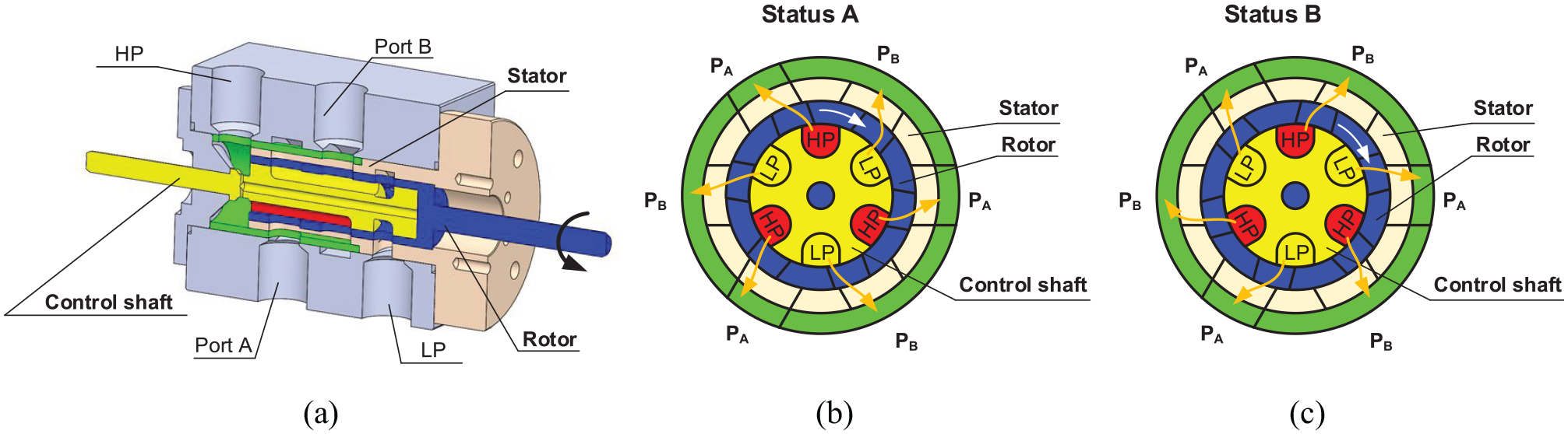
Section views of the rotary valve: (a) the axial section view of the rotary valve, (b) the radial section view of status A: HP port connects to Port A and (c) the radial section view of status B: LP port connects to Port A.
Analysis of the switching orifice area
Varying overlapped orifice area
To analyse the effective switching orifice area of the valve, the changing overlapped orifice areas (dashed line) between the control shaft, the rotor and the stator are shown in Figure 3(a), through which the flow passes from the HP port on the control shaft to Port A on the stator. A 3D view of the valve assembly of the control shaft, the rotor and the stator is presented in Figure 3(b), which shows the flow crosses from control shaft slots to stator slots through rotor slots. The slots of the three components are unfolded to show the details of the overlapped changing orifice areas in 2D in Figure 3(c). It clearly shows the supply orifice area between the control shaft and the rotor As and the delivery orifice area between the rotor and the stator Ap, of which the radial lengths (Ls and Lp) and axial lengths (Hs and Hp) are changing with the movement of the rotor slot. The effective switching orifice area of the valve is dependent on the changing of As and Ap, therefore, the analytical calculation of Ls, Lp, Hs and Hp are required to calculate the switching orifice area.
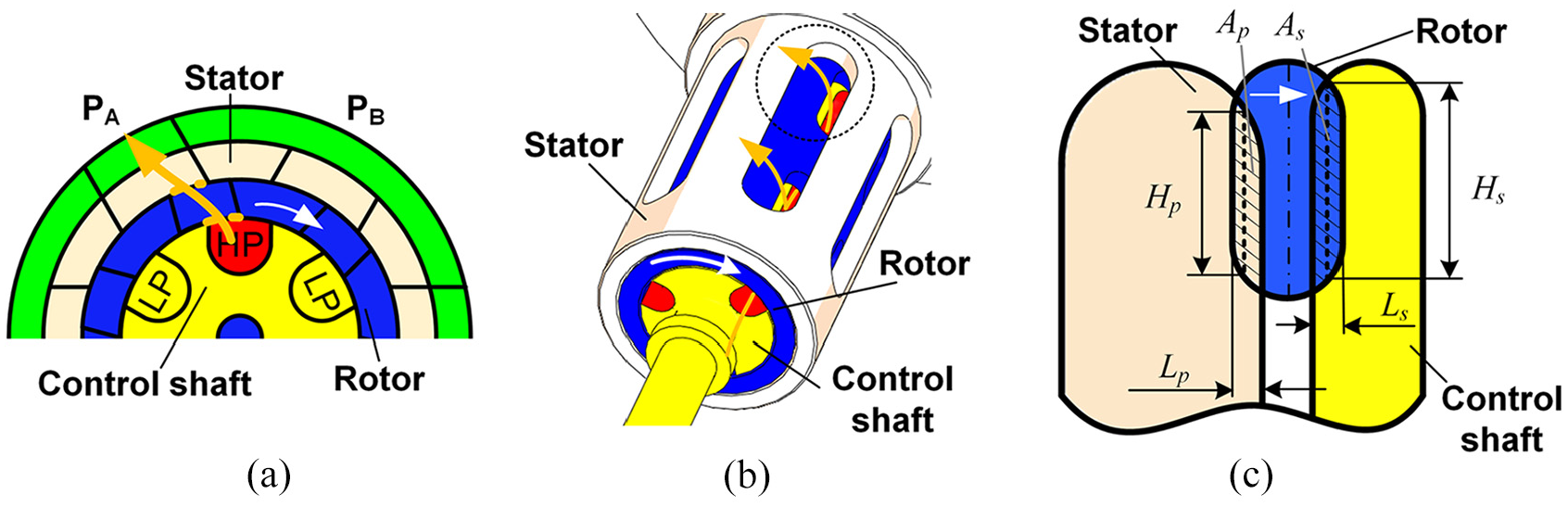
The changing overlapped orifice areas of the valve between the control shaft, the rotor and the stator (a) axial section view, (b) 3D view in the valve assembly and (c) unfolded 2D view.
Radial lengths
To simplify the analysis, the switching ratio
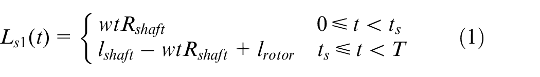
where
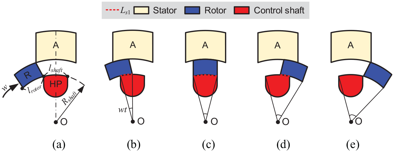
The variation of the radial length of the supply orifice area Ls1 at the switching ratio of 1: (a) t = 0, (b) 0 < t < ts,(c) t = ts, (d) ts < t < T and (e) t = T.
Figure 5 shows the variation of the radial length of the delivery orifice area Lp1 (dashed line) at the switching ratio of 1. Lp1 increases from 0 at t = 0 (Figure 5(a)) to the maximum value of lrotor (the arc length of the rotor slot) at t = tp1 (Figure 5(c)), remains constant until t = tp2 (Figure 5(e)), and then decreases to 0 at t = T (Figure 5(g)). The radial length of the delivery orifice area Lp1 for one switching cycle is given by equation (2)
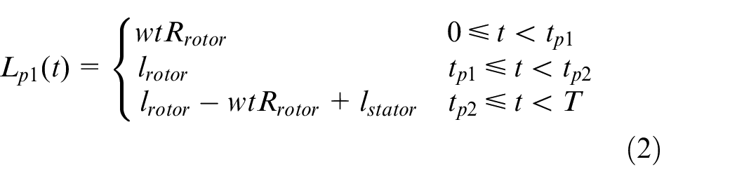
where
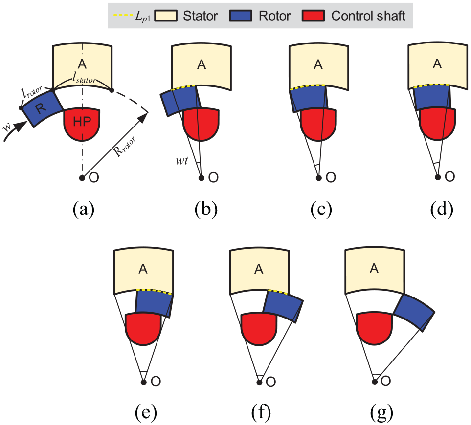
The variation of the radial length of the delivery orifice area Lp1 at the switching ratio of 1: (a) t = 0, (b) 0 < t < tp1,(c) t = tp1, (d) tp1 < t < tp2, (e) t = tp2, (f) tp2 < t < T and(g) t = T.
The relationship between the radian speed of the rotor w and the switching frequency f is given by equation (3)

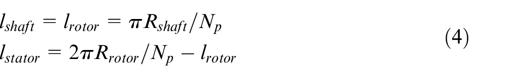
where Np = 6 is the number of the slots on the rotor, which means there are Np switching cycles in a revolution. The arc length of the slots of the control shaft lshaft, the rotor lrotor and the stator lstator can be calculated based on the valve geometry parameters
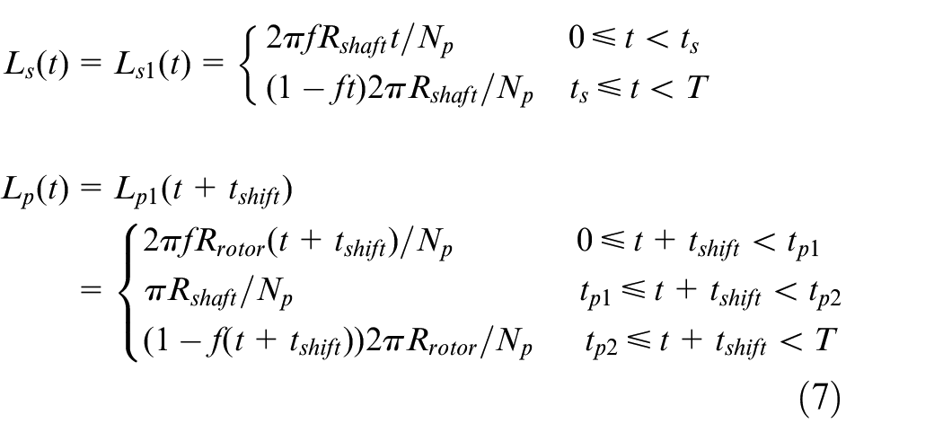
By substituting equations (3) and (4), equations (1) and (2) can be rearranged
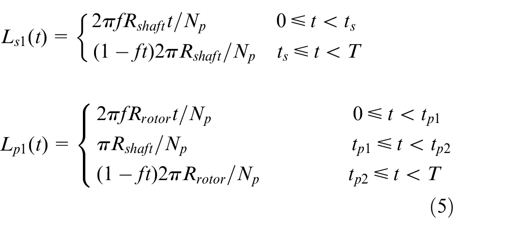
Using equation (5) and assuming the switching frequency of 100 Hz, the radial length of the supply orifice area Ls1 and the delivery orifice area Lp1 are shown in Figure 6.
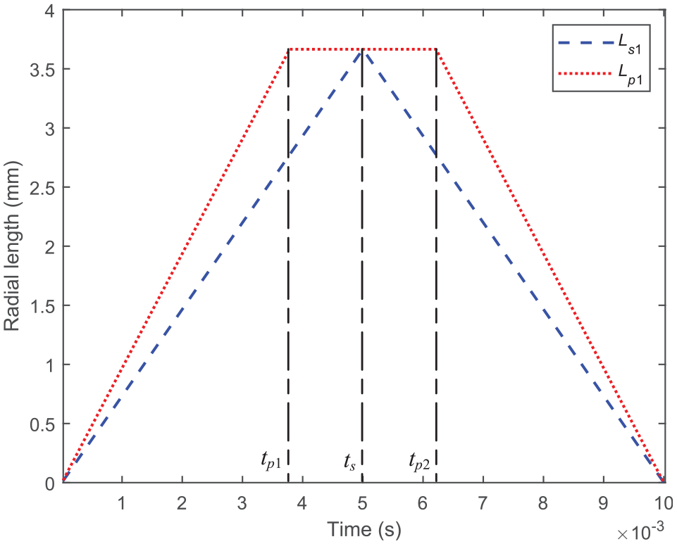
The radial length of the supply orifice area Ls1 and the delivery orifice area Lp1 at a switching ratio of 1 and a switching frequency of 100 Hz.
When the switching ratio
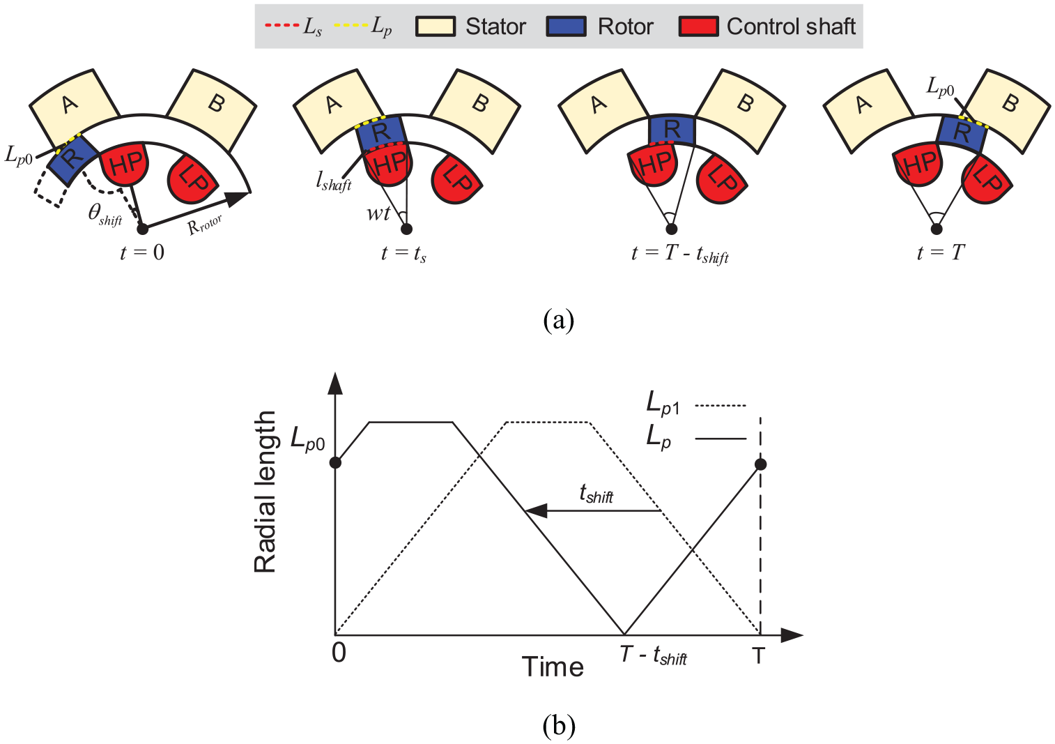
Variation of the radial length of the supply orifice area Ls and the delivery orifice area Lp: (a) variation of Ls and Lp at the switching ratio of

where
L s and Lp at a switching ratio of 0.5 and a switching frequency of 100 Hz are shown in Figure 8. For the first half cycle, the HP port opens to Port A when Ls increases from 0 at t = 0 and closes when Lp decreases to 0 at t = 0.005 s. For the other half cycle, the LP port opens to Port A with Lp increasing from 0 at t = 0.005 s and closes with Ls decreasing to 0 at t = 0.01 s.
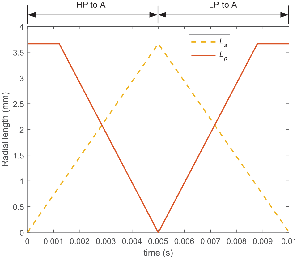
The radial length of delivery orifice area Lp and supply orifice area Ls at a switching ratio of 0.5 and a switching frequency of 100 Hz.
Axial lengths
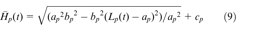
To investigate the axial length of the delivery orifice area Hp, the schematic diagram of the delivery orifice area Ap, which varies with the rotor movement in an unfolded view, is shown in Figure 9(a). The axial length of the delivery orifice area Hp is dependent on the radial length Lp, and the delivery orifice area Ap is the integral of Hp over Lp. To simplify the integral calculation, the orifice area Ap is considered equivalent to a rectangle (dashed line) with the width of Lp and the length of

where ap, bp and cp are the parameters related to the valve geometry.
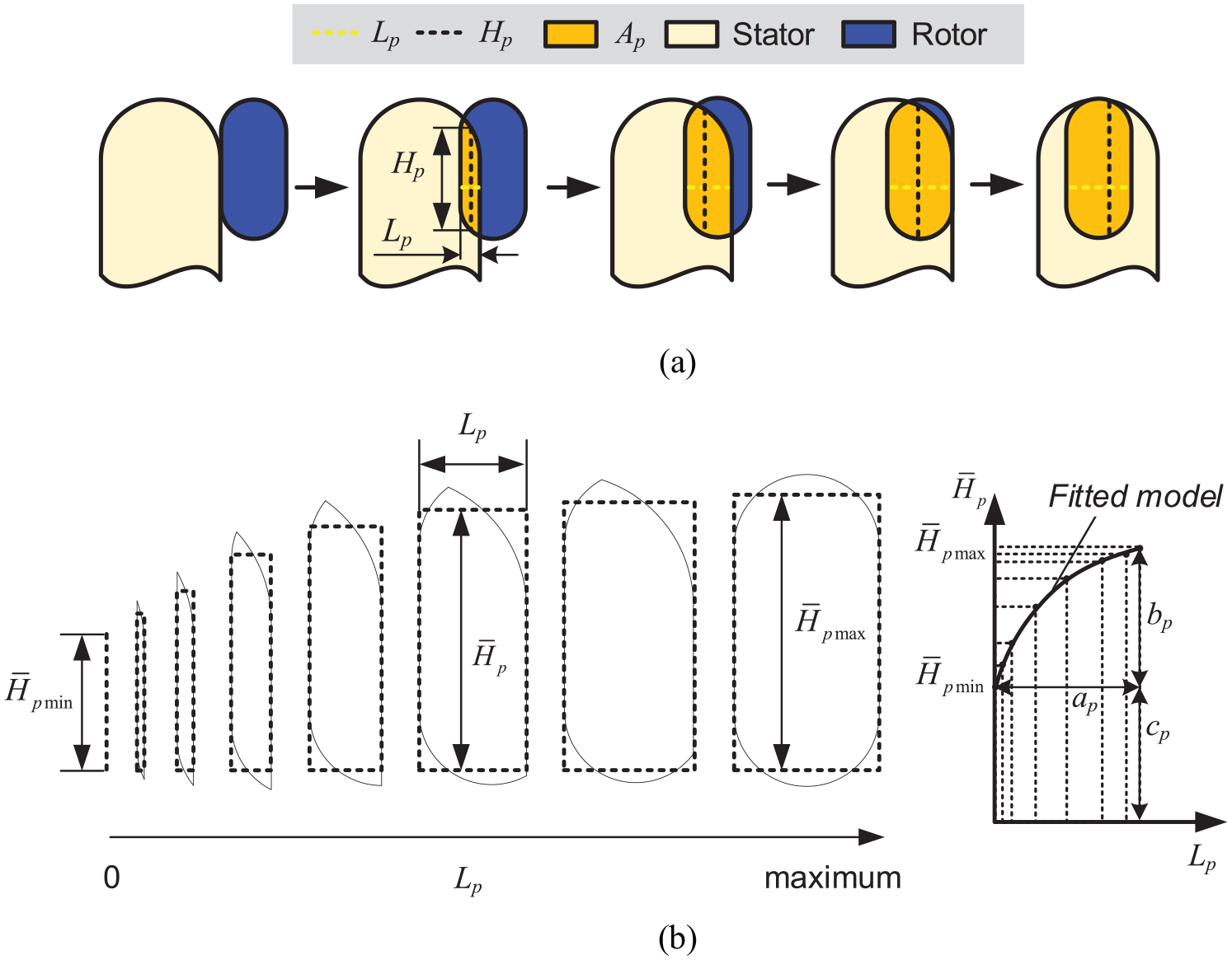
Analysis of the axial length of the delivery orifice area: (a) the variation of the delivery orifice area with the rotor movement and (b) modelling of the axial length of the delivery orifice area.
The same method is used for the approximation of
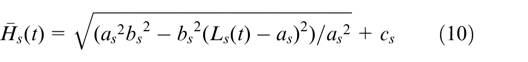
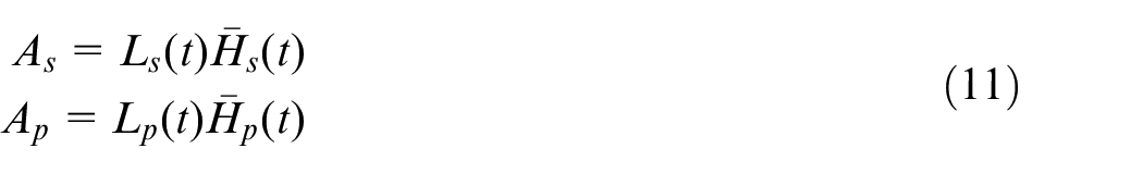
where as, bs and cs are the parameters related to the valve geometry. The supply orifice area As and delivery orifice area Ap can be calculated
Effects of valve body
In addition to the changing orifice areas, the effects of the valve body design on the switching orifice area of the valve are investigated. Figure 10(a) shows the flow from the HP port to Port A on the section view of the valve assembly including the control shaft, the rotor, the stator and the valve body. As can be seen from the arrows, the supply flow is branched into three flow paths. The flow of paths 1 and 2 sequentially crosses through the orifice area of the slot on the control shaft Ashaft, the supply orifice area As, the delivery orifice area Ap and the orifice area of the slot on the valve body Am to Port A. Unlike flow paths 1 and 2, the flow in path 3 crosses through the orifice area of the slot on the stator Astator to Port A after As and Ap without passing Am. When the rotor disconnects from the HP port and connects to the LP port, the flow from the LP port to Port A crosses the orifice areas in the same sequence due to the symmetric design of the rotor, the control shaft and the stator in the radial direction. The schematic arrangement of the orifice areas of the flow channels inside the valve from the HP/LP port to Port A is shown in Figure 10(b). Ad is the equivalent orifice area including the orifice areas in the dotted line where As and Ap are doubled because there are two rotor slots of each flow channel in the axial direction (see Figure 3(b)). When the HP port is connected, the flow from the HP port crosses into Ad and passing through Aout. When the LP port is connected, the flow goes through the orifice area ALP before crossing through Ad and Aout. ALP is the orifice area at the input of the LP supply and Aout is the orifice area at the output of Port A, which are constant and related to the geometry of the valve body.
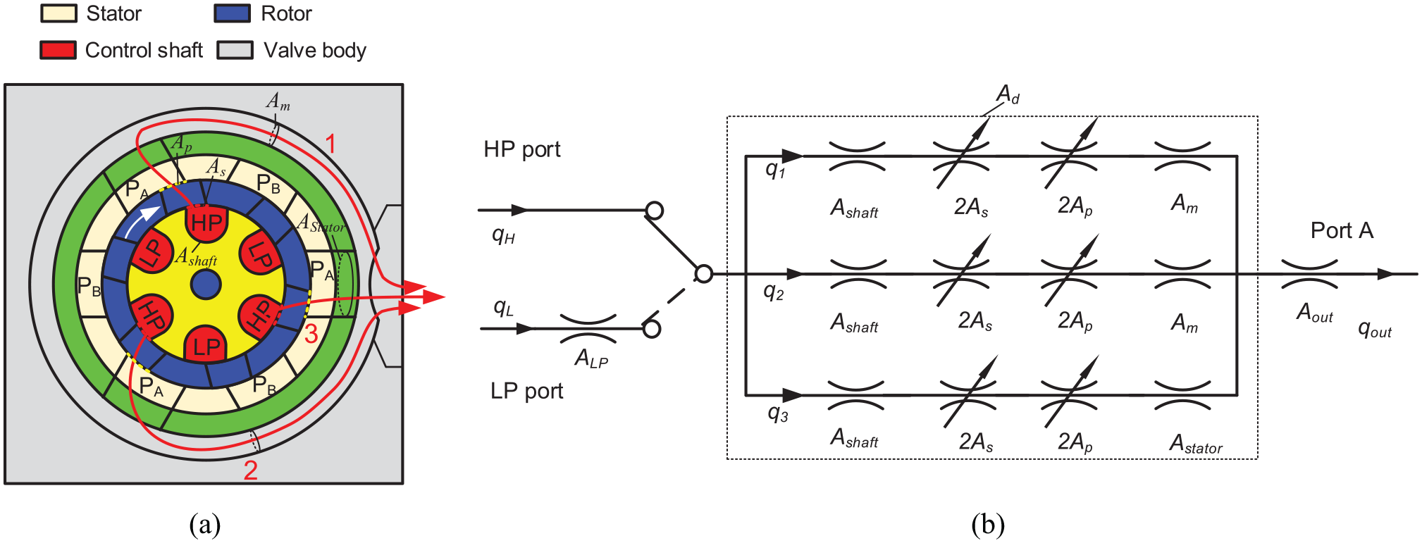
Effects of the design of the valve body on the switching orifice area of the valve (a) the supply flow from the HP port to Port A and (b) the schematic arrangement of the orifice areas from the HP/LP port to Port A.
The valve switching orifice areas from the HP/LP port to Port A denoted as AHA and ALA can be calculated by
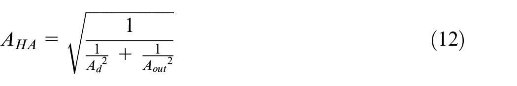
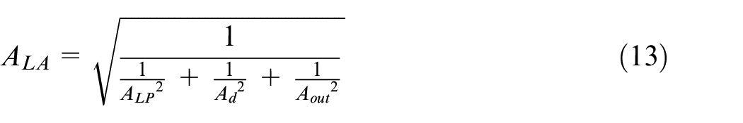
where Ad can be obtained by
Effects of valve leakage
The orifice areas from the HP port to Port A (AHA) and the LP port to Port A (ALA) should become zero at the middle point of a switching cycle when the radial length of delivery orifice area Lp is zero. However, this is not true in practice because the clearance between surfaces forms the leakage areas Aleak_HP and Aleak_LP when the HP or LP port is closed. The leakage areas are experimentally tested and assumed constant, which are considered as the minimum orifice areas from HP/LP port to Port A, as given by equations (15) and (16)
The switching orifice areas at a switching ratio of 0.5 and a switching frequency of 100 Hz are shown in Figure 11. The parameters used for the calculation are listed in Table 1. The switching orifice area from the HP port to Port A increases from 0.18 to 23.5 mm2 and decreases to 0.18 mm2 before the valve switches to the LP port. The switching orifice area from the LP port to Port A increases from 0.11 to 20.1 mm2 before decreasing to 0.11 mm2 at the end of the switching cycle. The transition time is defined as the time for the valve to switch from fully open to the HP port to fully open to the LP port, which is about 1 ms as shown in Figure 11. The orifice area of 15 mm2 is the critical point for the HP and LP ports being fully open.
The calculated valve switching orifice areas over a switching cycle at a switching ratio of 0.5 and a switching frequency of 100 Hz.
Parameters for calculation of the valve switching orifice areas.

HP: high pressure; LP: low pressure.
Transition throttling and compressibility effects
Theoretical analysis
When the high speed rotary valve switches from the HP port to the LP port, the pressure drop occurs during the switching transition which results in throttling energy loss. In addition, the density of the compressible fluid in the switched volume changes due to the pressure change. The throttling and compressibility effects can be combined and analysed to improve accuracy by modelling the variable pressure and flow rate in a switched volume 19 which can be modelled by
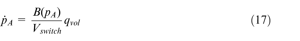
where pA is the pressure of the switched volume and also the pressure at Port A of the valve, Vswitch is the switched volume, qvol is the flow rate into the switched volume, B is the fluid bulk modulus which is dependent on pressure and can be represented by the model developed by Yu et al. 20
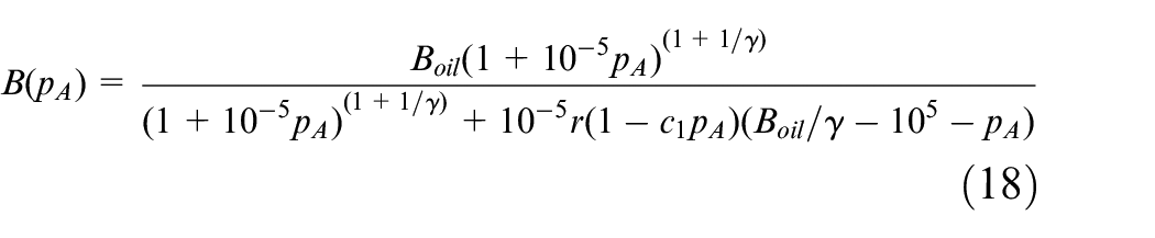
where Boil is the bulk modulus of hydraulic oil with no air, r is the volumetric ratio of air entrained in the oil/air mixture, c1 is a constant related to the effect of air dissolving into/out of solution and γ is the ratio of specific heats for an ideal gas.
There are two inlets and one outlet in the switched volume and the flow rate to the switched volume qvol is given by

where qHP-A and qLP-A are the flow rates through the HP port to Port A and through the LP port to Port A in the valve, qA is the delivery flow at Port A of the valve. qHP-A and qLP-A are described by the orifice equations with variable orifice areas AHP-A and ALP-A as
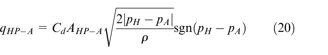
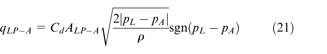
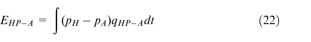
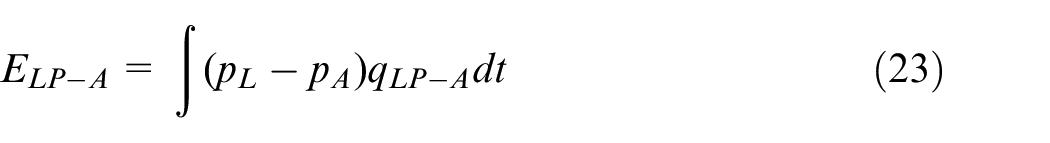
where Cd is the discharge coefficient, ρ is the fluid density, pH and pL are the high- and low-supply pressure, AHP-A and ALP-A are time-varying and dependent on the valve geometry as analysed in previous section. The throttling energy losses from the HP and LP port to Port A denoted as EHP-A and EHP-A can be obtained by
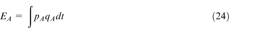
The output energy of the valve EA and the valve volumetric efficiency η can be calculated as

Effects of varying entrained air and switched volume
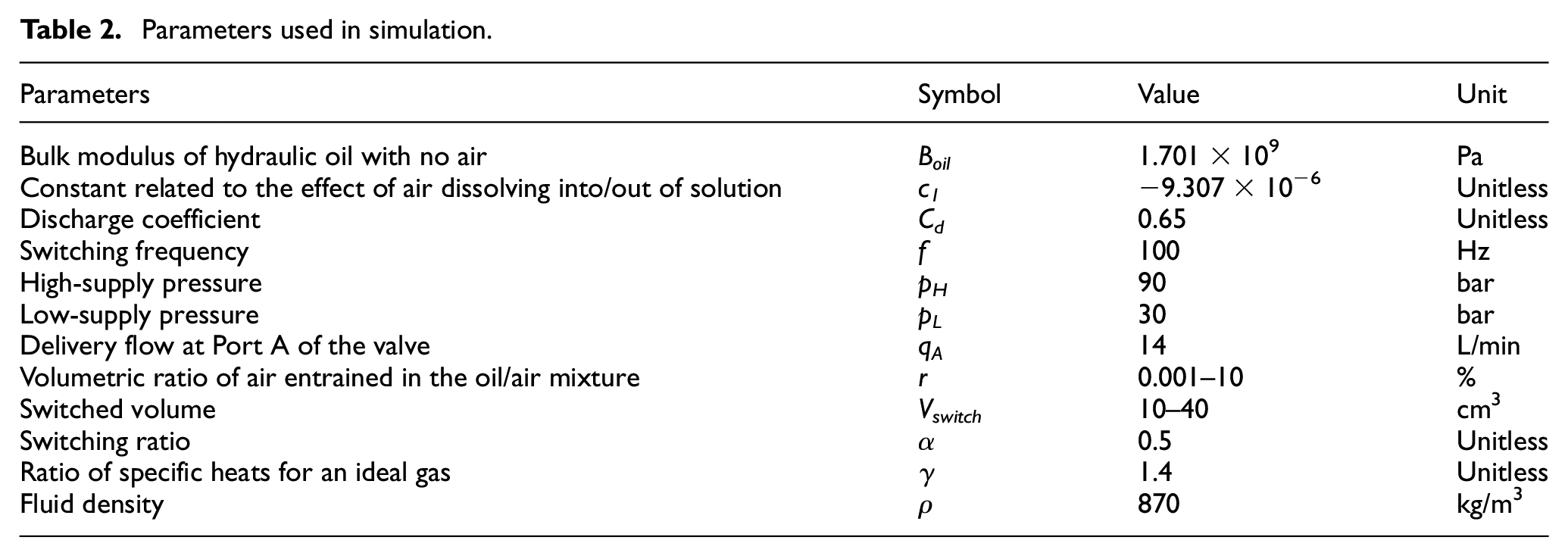
The effects of the entrained air and switched volume on the throttling energy losses, output energy and the volumetric efficiency of the valve are investigated in MATLAB/Simulink with the parameters listed in Table 2. The simulations are conducted with the volumetric ratio of air entrained in the oil/air mixture (entrained air ratio) between 0.001% and 10% and the switched volume between 10 and 40 cm3. The high-pressure supply is 90 bar and the low-pressure supply is 30 bar.
Parameters used in simulation.
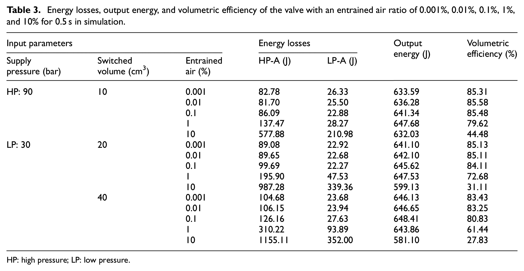
The model was conducted in MATLAB/Simulink for 0.5 s and the results are presented in Table 3. The switched volume was defined as 10, 20 and 40 cm3 to examine the effect of the size of switched volume. The entrained air of 0.001%, 0.01%, 0.1%, 1% and 10% were used to analyse the effect of fluid compressibility. It is found that the throttling energy loss from HP-A contributes about 3–5 times of energy loss than that occurred from LP-A. The volumetric efficiency of the valve varies from 27.83% to 85.58%. The minimum volumetric efficiency of the valve occurs with the largest switched volume of 40 cm3 and the highest entrained air ratio of 10%, which results in the highest fluid compressibility. In contrast, the valve achieves the maximum volumetric efficiency with the lowest switched volume of 10 cm3 and the lowest entrained air ratio of 0.001%, leading to the lowest fluid compressibility. With an increase of the switched volume, the throttling energy losses of HP-A and LP-A increase hence the volumetric efficiencies decrease. The volumetric efficiency reduces from 44.48% to 27.83% when the volume increases from 10 to 40 cm3 at the entrained air ratio of 10%. The effect of the entrained air ratio on the volumetric efficiency is small within the ratio range between 0.001% and 0.1%. When the entrained air ratio increases from 0.1% to 10%, the throttling energy losses of HP-A and LP-A significantly increase. For example, with a switched volume of 20 cm3, the energy loss from HP-A increased from 99.69 to 987.28 J, and the energy loss from LP-A increased from 22.27 to 339.36 J. The volumetric efficiency significantly reduced from 72.68% to 31.11%. This shows the fluid compressibility has significant effect on the energy losses and volumetric efficiencies of the valve.
Energy losses, output energy, and volumetric efficiency of the valve with an entrained air ratio of 0.001%, 0.01%, 0.1%, 1%, and 10% for 0.5 s in simulation.
HP: high pressure; LP: low pressure.
Computational fluid dynamics analysis
Computational fluid dynamics (CFD) is used to explore the pressure and flow characteristics of the valve in steady and dynamic states, the pressure losses of different parts in the valve and the effect of the fluid compressibility on the performance of the valve.
CFD modelling
The CFD analysis was conducted using Ansys/Fluent. The CAD model of the valve assembly was used to extract the flow channel (see Figure 12) inside the valve by logic operations on the rotor, the control shaft, the stator and the valve body. The flow channel comprises the stator channel, the rotor channel and the control shaft channel. The leakage channels between the control shaft, the rotor and the stator are modelled by two annular shapes as shown in Figure 12 to simplify the CFD calculation.
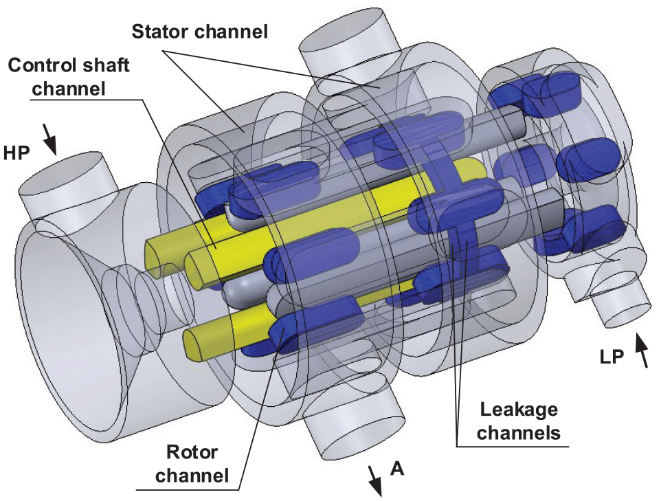
The flow channel inside the valve.
To determine a suitable mesh element size, a series of element sizes from 0.1 to 1 mm were used to conduct steady-state analysis. The results of the delivery pressure showed less than 0.05% difference of using the meshes with different sizes. Therefore, the flow channels were meshed at the element size of 1 mm to minimise the computation time with acceptable accuracy. The pre-processed and meshed flow channels were used to conduct steady-state and dynamic calculations.
For boundary conditions, the HP and LP ports were set to the pressure inlet type with constant pressures of 90 and 30 bar, respectively, and Port A was set to be the flow outlet type with a constant flow rate of 14 L/min. The stator and the control shaft channel were set to be stationary. The rotor channel was set to be stationary at different positions for steady-state analysis and to be rotating at a speed determined by the required switching frequency for dynamic analysis. The fluid flow pattern needs to be determined which can be estimated based on the Reynolds number. For the studied flow rate range (6–21 L/min) and the flow channel geometry, the Reynolds number value varies from Re = 3800 to Re = 5092 as calculated by
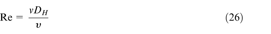
where v is the velocity of the fluid, DH is the hydraulic diameter (9 mm for the HP port and Port A, 5 mm for the LP port),

The fluid compressibility is considered in CFD modelling using simplified Tait equations which establish a nonlinear relationship between the density of liquid and the pressure under isothermal conditions by assuming the bulk modulus is a linear function of pressure. 25 This is readily implemented in Ansys/Fluent as following 26
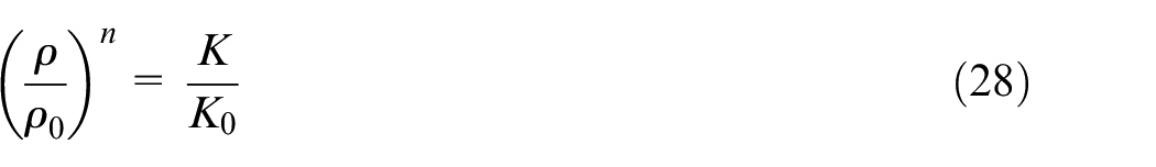
where
CFD results
Valve steady-state results
For steady-state analysis, the rotor channel was fixed at different positions. A certain relative position is used and results in 1.2°, 14.4° and 44.4° of a switching cycle (60°), representing the three stages including the HP port partly (3%) open to Port A during transition, the HP port fully open to Port A and the LP port fully open to port A. Figure 13 shows the CFD streamlines coloured with pressure, the velocity contours and velocity vectors (projected on the section plot) of the flow in the valve for the three stages in steady-state analysis.
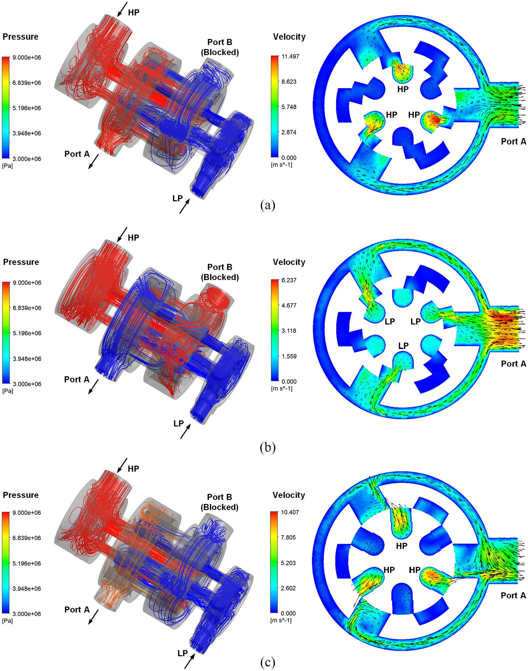
The CFD streamlines, velocity contours and velocity vectors of the flow in the valve at three stages in steady-state analysis: (a) HP port fully open to Port A, (b) LP port fully open to Port A and (c) HP port partly (3%) open to Port A during transition.
When the HP port is connected to Port A as in Figure 13(a), the flow streamlines show that the HP flow at 90 bar flows to Port A through the slots on the control shaft while the LP flow at 30 bar fills in the channels to Port B which is blocked. The velocity contour shows the three flow paths from the HP port to Port A. The flow velocities are very high in axial direction at the three slots on the control shaft due to the throttling effect. The flow velocity at the slot directly connected to Port A is much higher (up to 11.497 m/s) than that of the other two slots (up to 9 m/s) which means more flow crosses through this path due to the smaller resistance. The direction of flow changes from axial to radial to go through the overlapped orifice areas; hence, the axial velocity decreases while the radial velocity increases as the velocity vectors show. When the LP port is fully connected to Port A in Figure 13(b), the flow from the LP port at 30 bar exits at Port A while the flow from the HP port at 90 bar is blocked in Port B. Due to the low pressure of 30 bar, the flow goes through the flow channels with a lower velocity range (0–6.237 m/s), as shown by the velocity contour. The velocity difference between the three slots on the control shaft are less significant in this scenario due to the leakage flow from the HP port to the LP port which shows a velocity of about 1.5 m/s in the three blocked slots. Figure 13(c) shows the HP port is partly (3%) connected to Port A in transition stage. The streamline shows the pressure drops from 90 bar at the HP port to about 84 bar at Port A due to the extremely small orifice area (1 mm2) between the slots of the rotor and the stator. The maximum velocity of the fluid reaches 10.407 m/s as shown by the velocity contour in transition.
Valve dynamic results
For dynamic analysis, the rotor was set to rotate at the speeds between 52.36 and 314.16 rad/s corresponding to the switching frequencies ranging from 50 to 300 Hz. Figure 14 shows the streamlines coloured with pressure, the velocity contours and velocity vectors of the flow in the valve for the three stages in a switching cycle at a switching frequency of 100 Hz (104.72 rad/s).
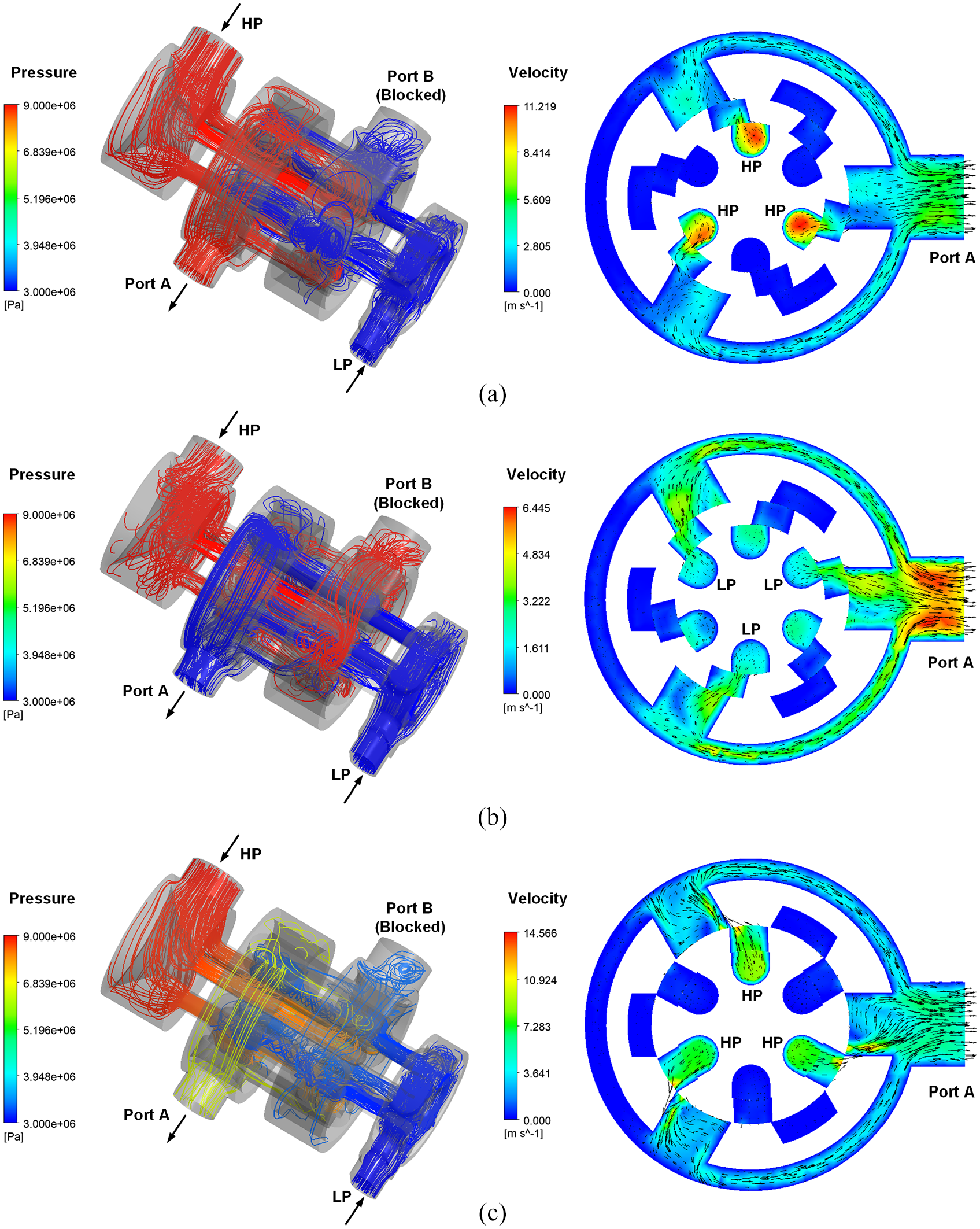
The streamlines, velocity contours and velocity vectors of the flow in the valve at three stages with a switching frequency of 100 Hz (a) HP port fully open to Port A, (b) LP port fully open to Port A and (c) HP port partly (3%) open to Port A during transition.
For the stages of the HP port and LP port fully connected to Port A (Figure 14(a) and (b)), the flow in the blocked channels shows a higher velocity in the dynamic state than that in the steady state, which shows the effect of the fluid inertia due to the motion of the rotor. During the transition, as shown in Figure 14(c), the pressure loss between the HP port and Port A and the maximum velocity of the flow significantly increases to 25 bar and 14.566 m/s compared to 6 bar and 10.407 m/s in the steady state. This can be caused by an increased flow force and friction due to the spinning of the rotor. The valve energy loss during the transition (switching loss) could be high due to the large pressure drop (25 bar) compared with the stages where the HP or LP ports are fully connected to Port A (<2 bar); therefore, the transition time should be as short as possible to achieve high energy efficiency.
The pressure losses of different parts in the flow paths 1, 2 and 3 of the valve (see Figure 10) were investigated in terms of the switching frequency. Figure 15 shows the pressure losses across the three flow paths (path 1, 2 and 3) at different stages of the valve with the switching frequency from 0 to 300 Hz with a step of 50 Hz. The results of flow path 1 and 2 are very close because of the identical structure; hence, only the results of flow path 1 are presented for flow paths 1 and 2. The total analytical pressure loss calculated using the standard orifice equation and the steady-state results without switching (0 Hz) are used to calibrate the discharge coefficients Cd and as a reference line.
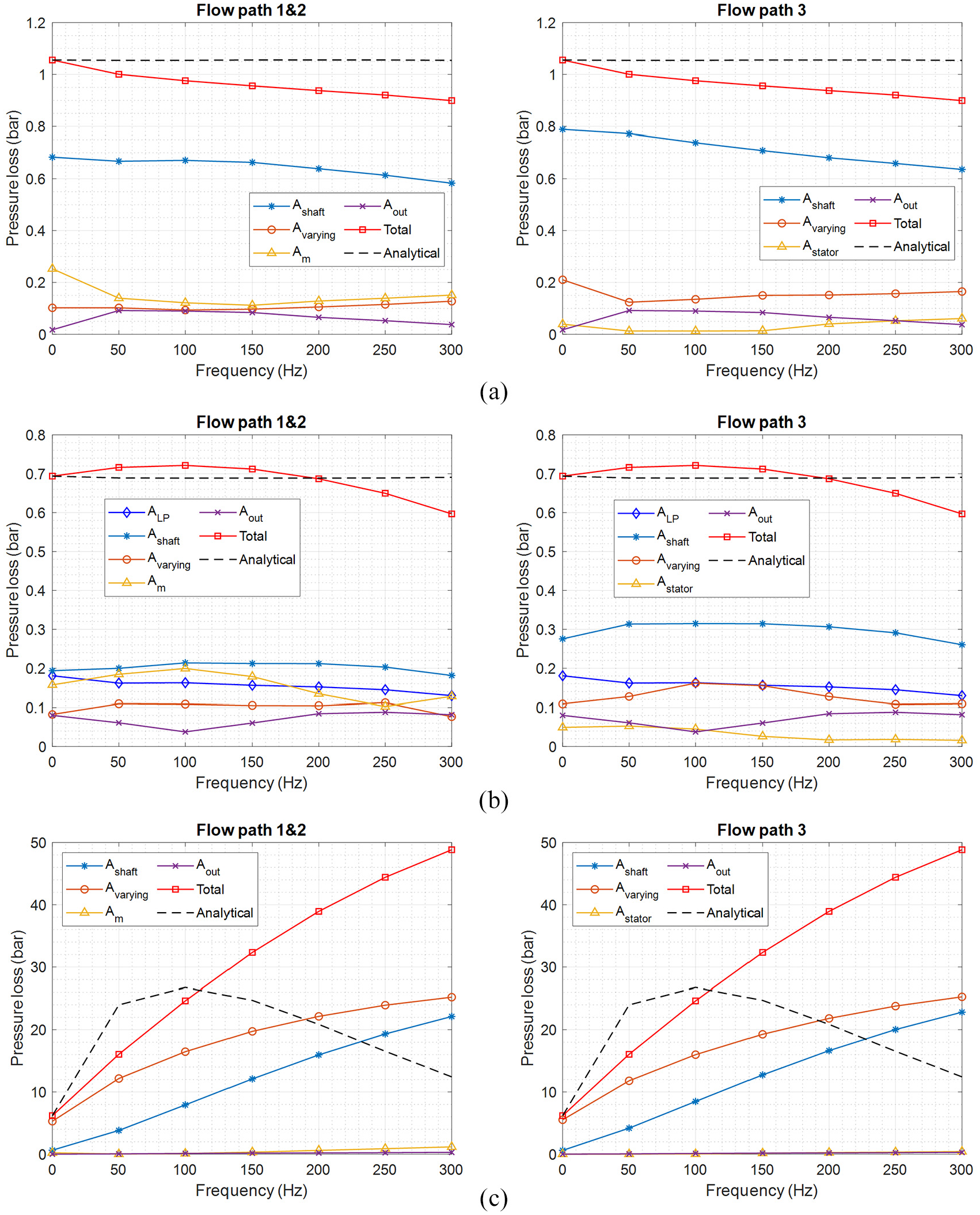
The pressure losses of different parts of the valve at three stages with the switching frequencies from 0 to 300 Hz with a step of 50 Hz (a) HP port fully open to Port A, (b) LP port fully open to Port A and (c) HP port partly (3%) open to Port A during transition.
When the HP port is fully connected to Port A, the total pressure loss decreases from 1.02 to 0.9 bar with the switching frequency from 0 to 300 Hz for flow paths 1, 2 and 3, as shown in Figure 15(a). The pressure loss from the slots on the control shaft (Ashaft) accounts for about 65% of the total pressure loss for flow path 1 and path 2 and 80% for flow path 3. This is because the orifice area of the slot on the valve body for flow path 3 (Astator = 50.93 mm2) is much larger than that for path 1 and path 2 (Am = 21.20 mm2). Therefore, the pressure drop across Astator (0.05 bar) is less than that of Am (0.2 bar). The total pressure loss drifts from the analytical result and the deviation increases to the maximum of 0.1 bar (10%) at 300 Hz.
When the Port A is fully connected to LP port, the total pressure loss increases slightly from 0.7 to 0.72 bar and then drops to 0.6 bar with the increase of switching frequency from 0 to 300 Hz for the three flow paths, as shown in Figure 15(b). The pressure loss across Ashaft accounts for 30% of the total pressure loss for the flow paths 1 and 2 and 40% for the flow path 3. The pressure drop across Astator of flow path 3 is 0.1 bar less than that of Am at flow paths 1 and 2.
During the switching transition as shown in Figure 15(c), the orifice area (Ashaft) and the varying orifice area (Avarying) cause significant pressure losses which increase from 0.6 to 23 bar and from 5 to 24.6 bar, respectively, with the switching frequency from 0 to 300 Hz for the three flow path, while the pressure loss across Am, Astator and Aout are negligible (<0.5 bar). The analytical total pressure loss increases from 6 bar at 0 Hz to about 25 bar for 50–150 Hz and decreases back to 12 bar for the three flow paths. This is because the delivery flow rate during the switching transition significantly increases to about 21 L/min for 50–150 Hz and decreases to 16 L/min at 300 Hz, compared to that of 14 L/min at the steady state. The total pressure loss from CFD results increases from 6.2 to 48.8 bar with the increase of the switching frequency. The slot on the control shaft (Ashaft) contributes to the significant part (30%–80%) of total pressure loss of the valve for all flow paths at three stages, which indicates that the pressure loss of the valve could be effectively reduced by increasing Ashaft.
Compressibility effect in CFD
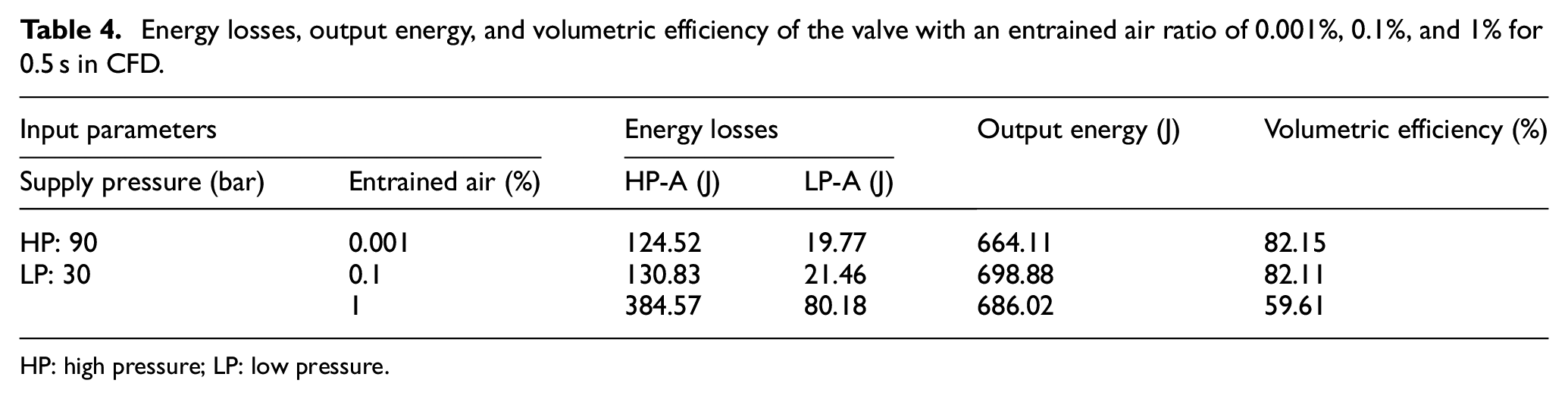
Compressibility is the measure of the change in volume a substance undergoes when a pressure is exerted on the substance. The bulk modulus of a liquid is related to its compressibility, which is defined as the pressure required to cause a unit change of volume of a liquid. The entrained air ratio is defined as the volumetric ratio of air entrained in the hydraulic oil/air mixture which can significantly affect the bulk modulus of the hydraulic oil used in the valve. To investigate the compressibility effect, the bulk modulus 1.6 × 10⁹ Pa, 2.1 × 10⁸ Pa and 2.4 × 10⁷ Pa at the reference pressure with the entrained air ratio of 0.001%, 0.1% and 1% are used. The switching frequency of the valve is 100 Hz, and the switching ratio is 0.5. The results of energy losses, output energy and volumetric efficiency of the valve with an entrained air ratio of 0.001%, 0.1% and 1% for 0.5 s in CFD are presented in Table 4. The energy losses and volumetric efficiency change slightly with the increase of the entrained air ratio from 0.001% to 0.1%. When the entrained air ratio further increases from 0.1% to 1%, the throttling energy losses of HP-A and LP-A significantly increase from 130.83 to 384.57 J and from 21.46 to 80.18 J, respectively, resulting in the decrease of the volumetric efficiency from 82.11% to 59.61%. This agrees well with the simulated results at the switched volume of 40 cm3 except for the slightly higher energy loss of HP-A, which could be caused by the friction loss in the CFD model.
Energy losses, output energy, and volumetric efficiency of the valve with an entrained air ratio of 0.001%, 0.1%, and 1% for 0.5 s in CFD.
HP: high pressure; LP: low pressure.
The CFD streamlines, velocity contours and velocity vectors of the flow with 1% entrained air in the valve at transition when the HP port is partly (3%) open to Port A are shown in Figure 16. With 1% entrained air, the pressure loss through the HP port to Port A increased to 56 bar and the maximum flow velocity increased to 24.8 m/s, which are about 24.6 bar and 14.6 m/s with a low entrained air ratio of 0.001% (see Figure 14(c)). In addition, the high fluid compressibility results in higher velocity of the leakage flow (up to 12 m/s) in the blocked channel as shown in the velocity contour and vectors, which can result in high flow loss. The simulated dynamic pressure of Port A, high-supply flow and low-supply flow of the valve from CFD models with the entrained air ratio of 0.1% and 1% are shown in Figure 17, where the pressure transition response at Port A is slower at 1% of entrained air ratio. This is because the switched volume entrains more air which increases the compliance of the system, and result in high-pressure loss during the transition. Moreover, with 1% entrained air, the dynamic flows fluctuated significantly during the transition and increased leakages occurred. This led to high flow losses. The high-pressure losses and flow losses during transition contributes to the high throttling energy losses and low volumetric efficiency, which is dependent on the fluid compressibility effect.
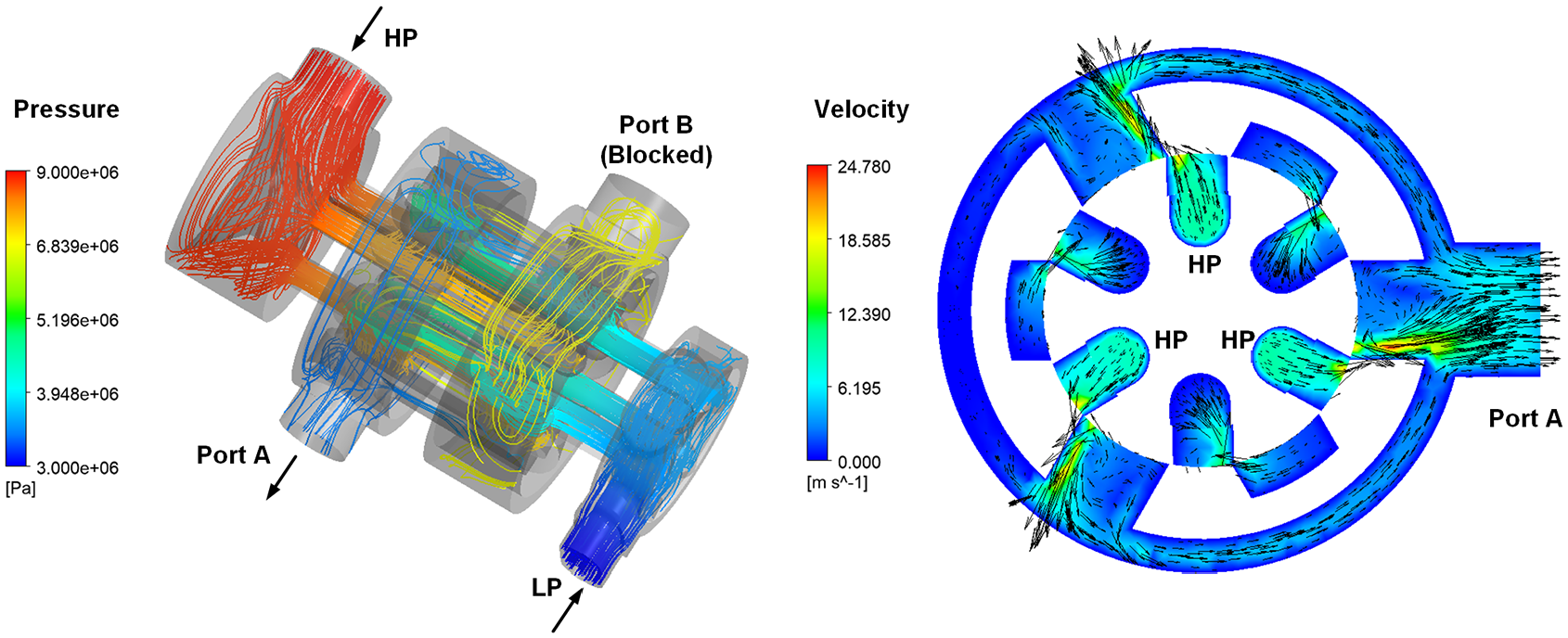
The CFD streamlines, velocity contours and velocity vectors of the flow with 1% entrained air in the valve at transition when the HP port is partly (3%) open to Port A.
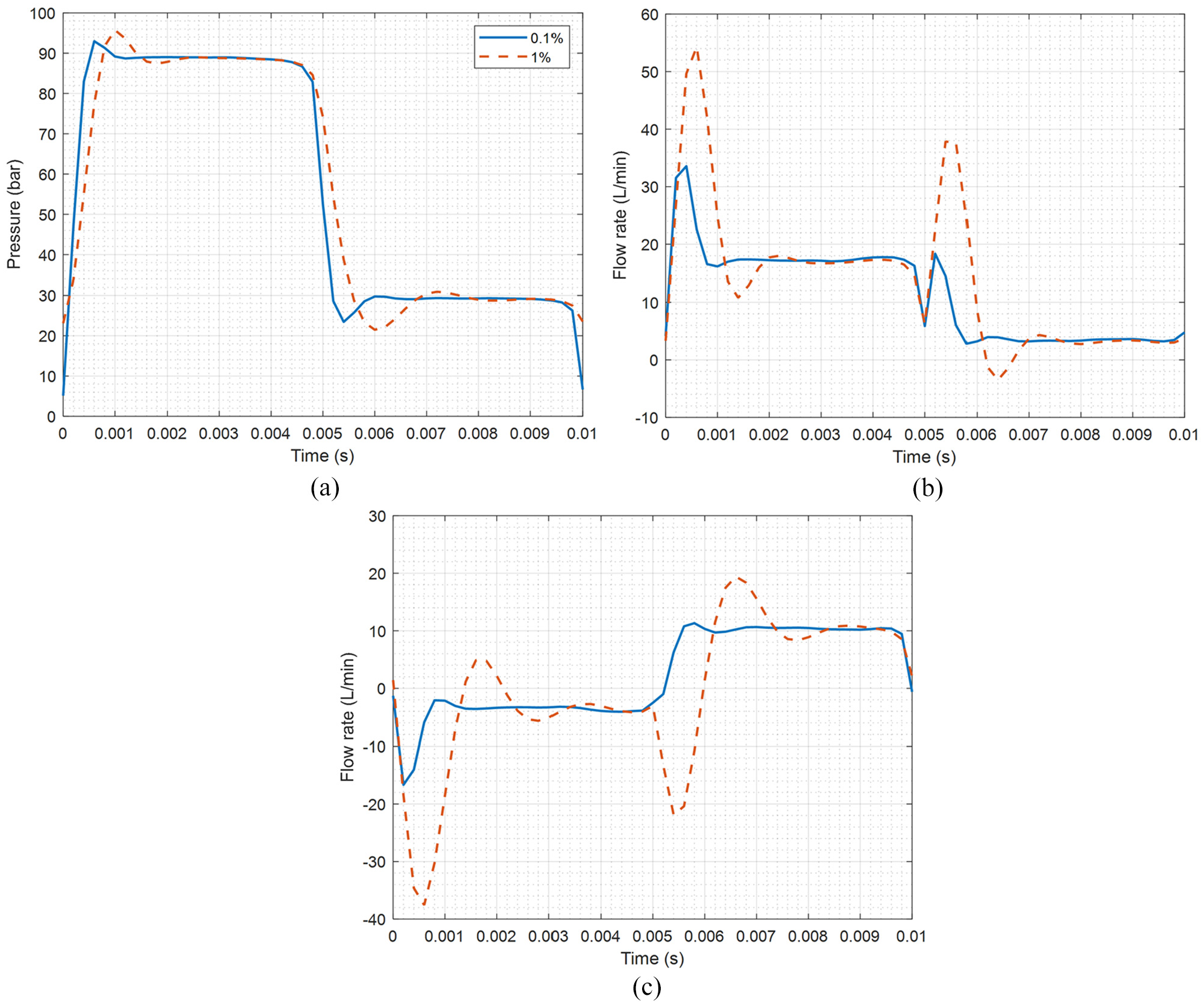
Dynamic pressure and flow rates at Port A, high-supply pressure port and low-supply pressure port, with 0.1% and 1% entrained air: (a) dynamic pressure at Port A, (b) dynamic flow at high-supply pressure port and (c) dynamic flow at low-supply pressure port.
Experimental validation
Experimental setup
An experimental testing rig shown in Figure 18 was used for investigating the steady and dynamic characteristics of the high-speed rotary valve. A hydraulic power pack including two gear pumps with a maximum supply pressure of 100 and 50 bar are used as HP and LP supplies. Three accumulators and three shock suppressors (Inline Pulse-Tone™ Shock Suppressors, Parker Hannifin) are used to eliminate the pressure pulsations. The charging pressures of the HP, LP and downstream accumulators are 45, 15 and 30 bar, and charging pressures of the shock suppressors are 22.5, 7.5 and 15 bar, respectively. A brushless servomotor (Baldor BSM50N-375AF) with a maximum speed of 5100 r/min is used to drive the rotor of the valve to control the switching frequency, and a stepper motor (stepIM NEMA34) is used to drive the control shaft to control the switching ratio. Three miniature piezoresistive dynamic pressure transducers (Measurement Specialties XP5 series) are used to measure the pressure of the HP port, the LP port and Port A of the valve. (The transducers ranges are from 0–350 bar, 0–35 bar and 0–200 bar, correspondingly.) A gear flow meter (0.5–70 L/min, ZHM series from KEM) was used to measure the dynamic HP supply flow rates. The delivery flow rate at Port A was measured using a turbine flow meter (HYDAC, 6–60 L/min).
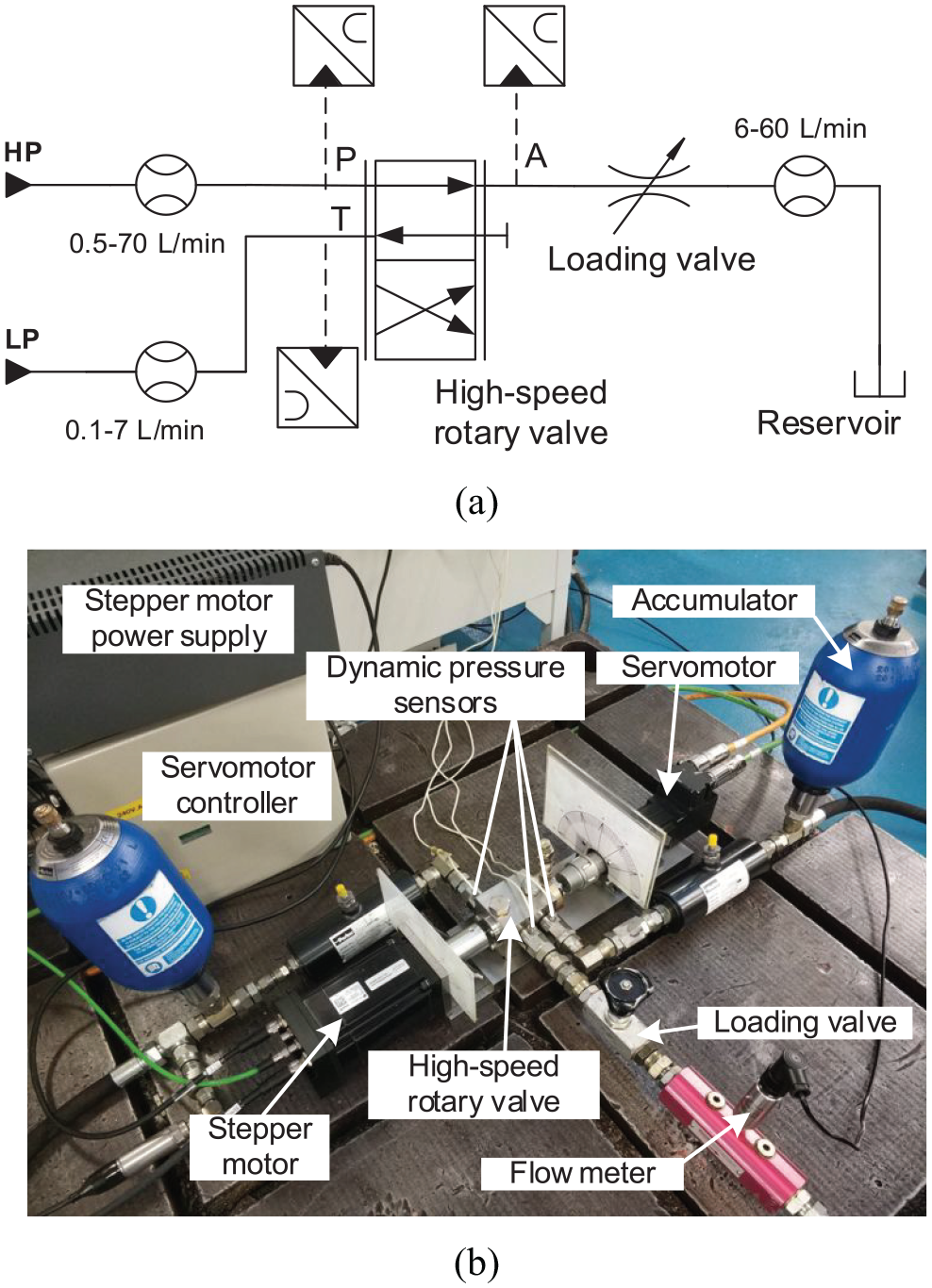
Experimental rig set up for steady and dynamic characteristics of the rotary valve: (a) schematic of the test rig and (b) photograph of the test rig.
Steady-state characteristics
The rotor is positioned to the maximum switching orifice area of the valve from the HP port to Port A for a steady-state characteristics test. Figure 19 shows the flow-pressure characteristics of the valve. Due to limited flow capability of the dual pump, the valve is tested at the flow rates range of 15–27 L/min with the pressure difference from 1.3 to 3.5 bar. Figure 19(a) describes the discharge coefficient as a function of the Reynolds number. The empirical model from Wu et al. 27 is used and the parameters are identified for discharge coefficient correlation, which is given by

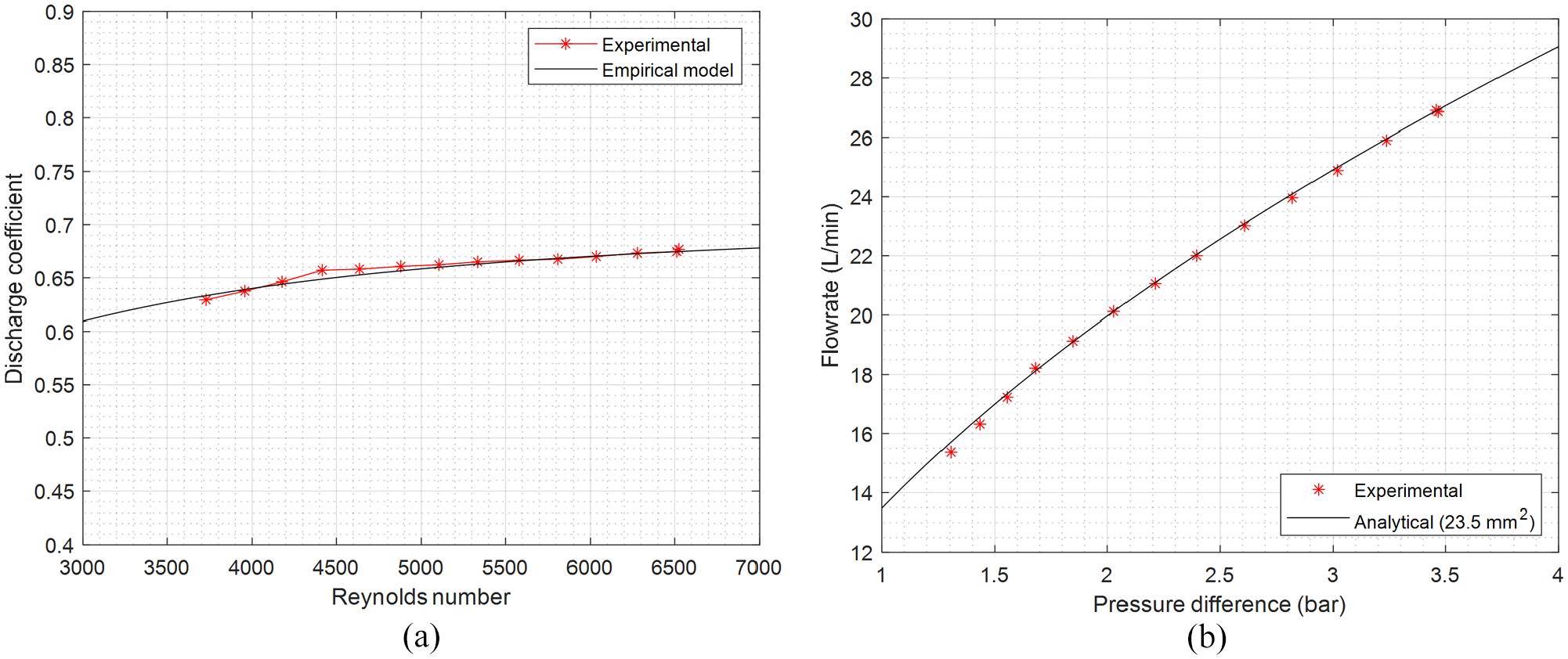
Steady-state flow-pressure characteristic of the maximum switching orifice area from the HP port to Port A: (a) discharge coefficient versus Reynolds number and (b) flow versus pressure difference.
The empirical model shows a very good match to the experimental results and can be used to obtain a correlated discharge coefficient. Figure 19(b) shows the relationship between the delivery flow rate and the pressure difference. It demonstrates the capability of the valve to deliver a flow rate of 20 L/min at a pressure drop of 2 bar. The analytical result is calculated using the orifice equation for an orifice area of 23.5 mm2 with the discharge coefficient correlation. Good agreement has been achieved between the analytical and experimental results.
The characteristic of the switching orifice area
The quasi-static experimental tests were conducted to validate the characteristics of the switching orifice area. The rotor was manually rotated from 0 to 60 degree in 2.5 degree increment with the control shaft fixed at the switching ratio of 0.5. Figure 20 shows the orifice areas from the HP and LP port to Port A, which are obtained from the analytical model, CFD analysis and experimental results. The experimental results agree very well with the analytical and CFD results and show that the leakage area of the valve is small (<0.2 mm2) when fully connected to the supply ports and relatively large (1–3.5 mm2) in transition.
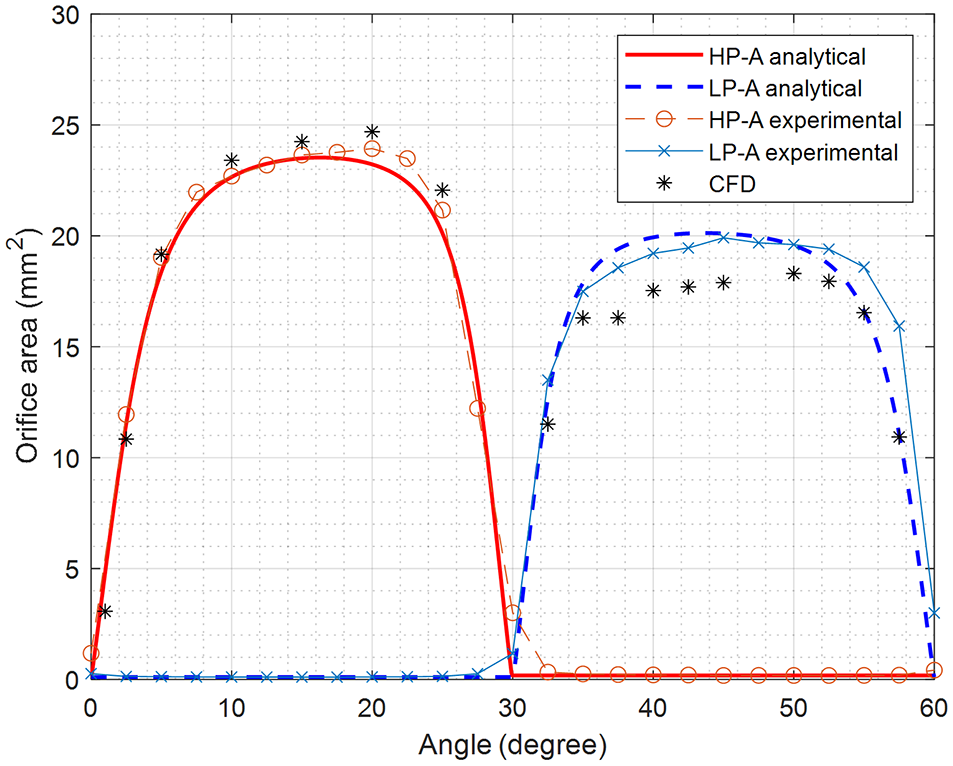
The switching orifice areas of analytical, CFD and experimental results.
Pressure dynamics of the rotary valve
The dynamic pressures at the delivery port (Port A) of the rotary valve were investigated experimentally with a high-supply pressure of 90 bar and a low-supply pressure of 30 bar. Figure 21 shows the simulated, CFD and experimental dynamic pressures at the delivery port (Port A) of the rotary valve, which agree well when the valve is fully open to the HP port or the LP port. High-frequency oscillations were observed during the experiments. This may be caused by the other effects of this highly dynamic test system, such as wave propagation effect along the connection hoses or system vibrations, which will be investigated in our continuing research.
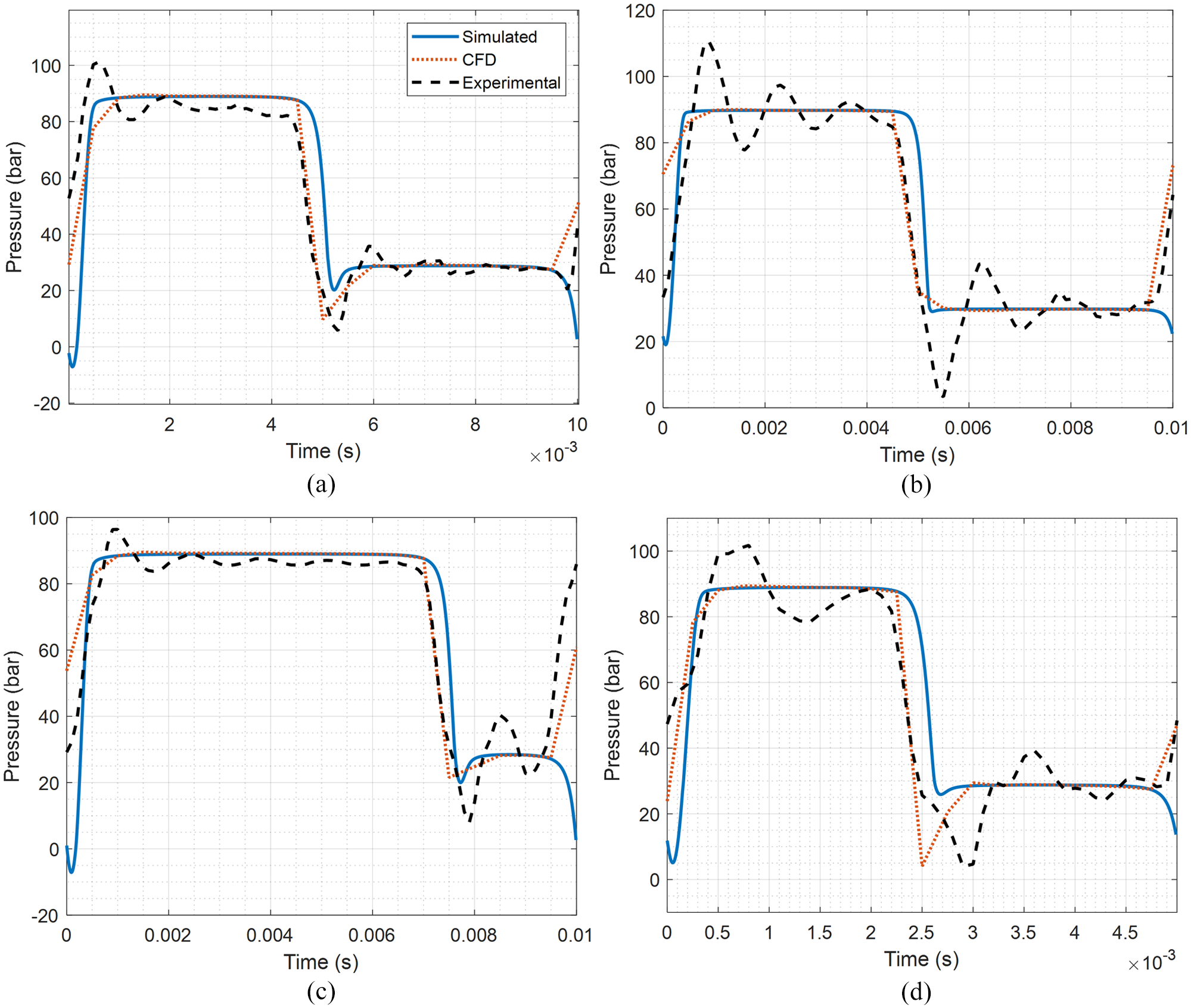
Dynamic pressures at the delivery port (Port A) of the rotary valve at various operating conditions: (a) 0.5 switching ratio, 14 L/min and 100 Hz; (b) 0.5 switching ratio, 6 L/min and 100 Hz; (c) 0.75 switching ratio, 14 L/min and 100 Hz; and (d) 0.5 switching ratio, 14 L/min and 200 Hz.
The CFD and experimental pressures switch from the high-supply pressure about 0.25 ms faster than that of simulated results, and the simulated pressure does not capture the increase of pressure when the LP port is closing at the end of the cycle due to the simplified simulation models. The experimental results show that the valve can achieve a transition time of about 1 ms from the high-supply port (90 bar) to the low-supply port (30 bar) for the flow rate of 6 and 14 L/min and the switching frequency of 100 and 200 Hz.
Discussion
In the investigation of the pressure dynamics of the valve, the delivery pressure drops to a very low value at the transition (see Figure 21) when the valve switches between the HP port and the LP port. This is because the switching orifice area of the valve reduces to the minimum (the leakage area) and a large pressure drop between the supply port and the delivery port is needed in order to maintain the delivery flow through such a small orifice area. When the LP port is connected, the supply pressure is low and the delivery pressure needs to be much lower than the low-supply pressure to achieve the desired pressure drop and maintain the delivery flow. In some cases, the delivery pressure would become negative if the low pressure was too low or the delivery flow rate was too high, which results in cavitation. In actual applications of SIHCs, the low-supply pressure can be boosted using a pressurised tank, and the maximum delivery flow can be limited accordingly to avoid cavitation. Moreover, the high-frequency damped oscillations are observed at the dynamic pressures of the delivery port (Port A). When operating the valve at high switching frequencies in SIHCs, the oscillations can cause large pressure ripples and high-frequency fluid-borne noises in the system. The oscillations could be caused by the fluid compressibility of the switching volume, the wave propagation effect of the connection hoses, damping in the supply lines and system vibration, which will be investigated in the future.
Conclusion
SIHCs can control pressure or flow and achieve high energy efficiency by digital switching instead of the dissipation of power by throttling. A high-performance switching valve is essential and its switching characteristics have significant effect on the energy efficiency of SIHCs. The switching characteristics of a high-speed rotary valve used for SIHCs are investigated by simulations, CFD analysis and experiments. The switching orifice area is analysed based on the movement of the valve rotor with a consideration of the design of the valve body, which shows a good agreement with CFD and experimental results. The transition throttling and compressibility are theoretically modelled and validated in CFD. The results show that high fluid compressibility causes high pressure and flow loss, which significantly increases the throttling energy and reduces the efficiency of the valve. The pressure dynamics of the valve when switching is modelled by considering the switching orifice, leakage and fluid compressibility, which is validated in CFD and experiments. The valve has shown promising performance, delivering 40 L/min at 10 bar pressure drop and switching at the maximum frequency of 317 Hz with a transition time of about 1 ms. The proposed theoretical and CFD models can assist the design and optimisation of digital high-speed rotary valves, which in turn is very useful for understanding, analysing and optimising the characteristics and performance of SIHCs in digital hydraulics.
Footnotes
Acknowledgements
The authors would like to thank Mr Xiaoming Chen’s contributions to CFD modelling.
Declaration of conflicting interests
The author(s) declared no potential conflicts of interest with respect to the research, authorship and/or publication of this article.
Funding
The author(s) disclosed receipt of the following financial support for the research, authorship and/or publication of this article: This research was supported by the RAEng/The Leverhulme Trust Senior Research Fellowship (grant number LTSRF1819\15\16), the RAEng Proof-of-Concept Award (PoC1920/15) and the China Scholarship Council PhD studentship (201706150102).