
Abstract
Gas compressors are critical yet energy-intensive components of pipeline networks. Accurately predicting their performance is a significant design and operational challenge, profoundly affected by the thermal behaviour of the transported gas. This study introduces a novel application of a techno-economic and environmental risk analysis (TERA) framework to determine gas compressor performance under three distinct gas flow temperature assumptions: isothermal, intermediate, and non-isothermal. The analysis, performed in MATLAB R2024a, integrates thermodynamic gas properties, pipeline hydraulics (via the Weymouth equation), and compressor characteristics, explicitly accounting for ambient temperature and altitude variations at each compressor station along the pipeline route. The results demonstrate that the common assumption of isothermal flow yields fixed but potentially inaccurate operating points. In contrast, non-isothermal analysis, which ties gas temperature to fluctuating ambient conditions, reveals significant operational dynamics. Specifically, compressor power demand peaks at 15:00 hours during the hottest season and reaches its lowest point at 06:00 hours during the coldest season, directly correlating with ambient temperature cycles. This fluctuation, which can critically impact design and fuel consumption, is entirely masked in isothermal and intermediate models. Furthermore, the findings show that for every 1% increase in the non-isothermal ambient temperature, the compressor suction pressure decreases by an average 0.1% and the compressor power demand increases by an average 0.3%, corresponding to an average increase of 0.3% in the polytropic head. A ±5% parametric sensitivity analysis confirms that inlet temperature exerts the strongest influence on power demand (±1.5%), followed by mechanical efficiency (±1.0%), pressure ratio (±0.8%), and gas composition (±0.4%). The total estimated annual operational cost for the 18-station pipeline network under isothermal conditions is approximately USD 90.66 million; however, a sensitivity analysis assuming a +10% increase in power demand during daily peaks reveals that operational costs could be underestimated by more than USD 56,000 per year for a single station, demonstrating that the isothermal assumption risks substantial under-estimation of long-term operational expenditures (OPEX). This study provides, for the first time, a comparative analysis of these three scenarios within a unified TERA framework, delivering crucial insights for selecting appropriately sized compressors. The MATLAB model was validated against Aspen HYSYS, showing excellent agreement with a maximum deviation of only 0.348% and a mean absolute deviation of 0.035% across all 18 stations. Therefore, this work offers a robust methodological advance that can assist designers in optimising the design and operation of existing or new long-distance natural gas transmission pipelines, leading to improved economic and operational outcomes.
Keywords
Introduction
Natural gas is a crucial fuel used in various industries and sectors of the economy. Its low carbon footprint compared to coal makes it a fuel of choice in countries where renewable energy and other alternative fuels are expensive to obtain. There is a need to transport this gas from surplus locations to areas in short supply. In many cases, these locations are usually thousands of kilometres apart. Therefore, it is imperative to design an efficient transportation system that meets end-user demands under all conditions. Natural gas transportation via pipeline has been identified as an economical and efficient means of gas transportation over long distances to areas with high demand.1–22 The properties and composition of natural gas significantly influence pipeline operating conditions. These depend on the annual extraction period, the source of production, and the degree of gas treatment.
23
Therefore, any change in the natural gas composition will ultimately affect its compressibility factor, gravity, density and other thermophysical properties. These pipelines require that the compressor stations be placed at appropriate distances. This is to ensure the continuous operation of the various components and meet end-users’ demands. These stations are thoughtfully positioned at regular intervals along the pipeline and require large areas of land.
24
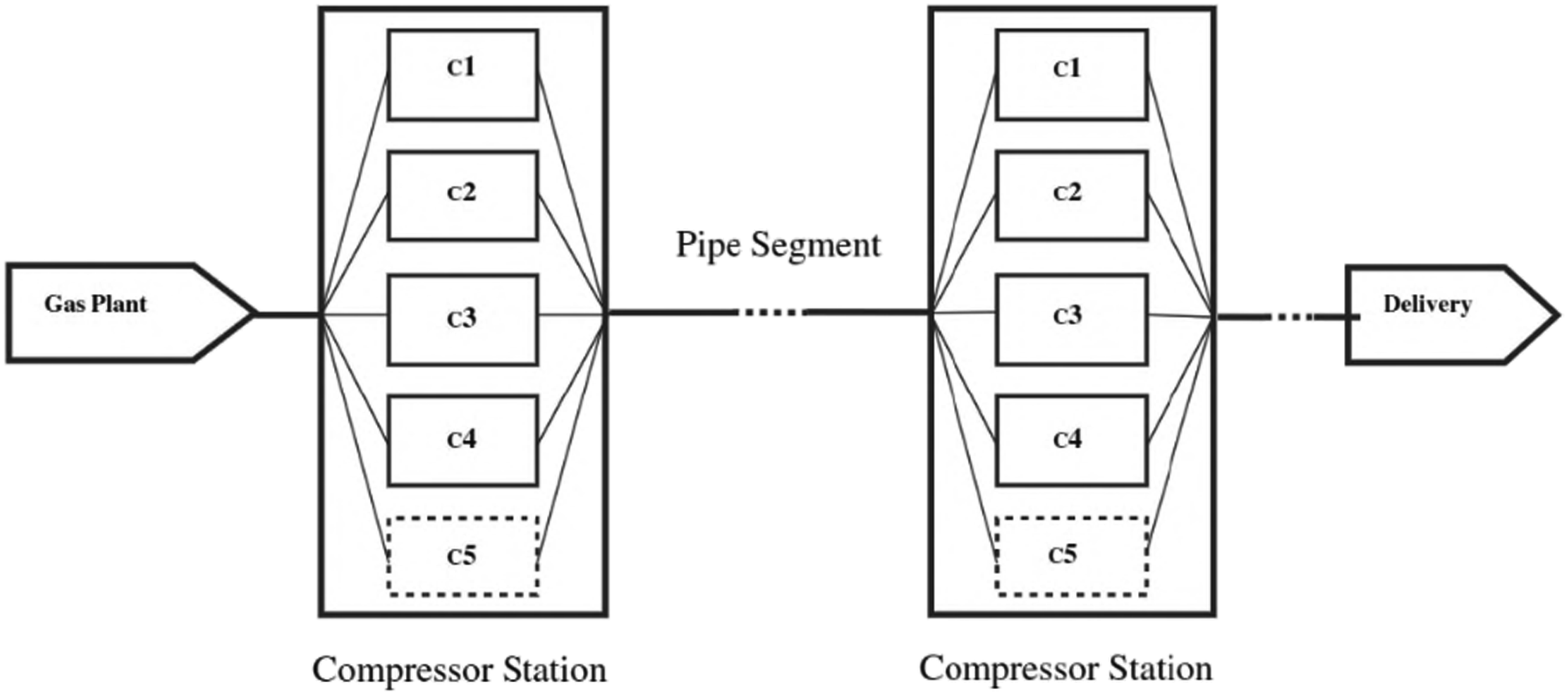
It is estimated that compressor stations consume about three to five per cent of the total gas transported.18,25 They accommodate compressors driven by prime movers and are usually installed some kilometres apart along the pipelines.26–30 Figure 1 illustrates the schematic diagram of the compressor station layout and pipe segments. It features five compressor units arranged in parallel at each station. This includes a gas plant supply node and a delivery terminal at the demand node. Compressor stations and pipe segments schematic.
31
Efficient design of compressor stations and pipeline systems is vital for meeting end-users’ demands and minimising transportation costs. After all, an efficient gas transmission network can reduce natural gas consumption at compressor stations by at least 20%.
25
The ambient conditions at the location influence the performance of compressor stations and pipeline systems, the flow rate, and the operation of compressor stations.
32
Hence, understanding the performance of gas compressors in natural gas transmission pipelines is essential for the efficient operation of the system and its components. Therefore, it is crucial to examine various parameters when designing compressor stations and pipelines. This includes ambient conditions, pipe diameter, length, elevation, natural gas properties, and gas compressor performance.
33
Nasir stated that the flow rates of the pipeline depend on factors such as pipe diameter, length, pressure drop from friction, gas suction temperature, suction pressure, and the properties of the gas.
34
Gas compressors are a crucial component of compressor stations and pipeline systems. They supply the pressure energy needed for a constant gas flow through the pipeline. Most long-distance transmission pipelines operate at pressures ranging from 60 to 100 bar. Therefore, it is imperative to compress natural gas to pipeline pressures.35–37 Natural gas compression is achieved by converting the driver’s mechanical energy to kinetic energy in the gas. Multiple gas compressors can be installed in either parallel or series configuration within a compressor station. This is to enhance the pipeline flow rate or increase the outlet pressure.
38
When choosing a compressor for a specific application, it is essential to consider factors such as performance, reliability, availability, and cost. Gas compression is an energy-consuming process since more than 67% of annual operating costs are usually used up by energy utilised for this process.
4
Thus, a minuscule enhancement in efficiency will significantly impact operating costs. After all, the economic success of a gas compression operation is dependent on gas compressor performance.27,39–42 The centrifugal compressor is preferred over other compressor types. This is due to its good performance, high availability, low operation and maintenance costs, simple construction, low head, and suitability for high-volume flows. Figure 2 shows Siemens’s barrel-type single-shaft pipeline centrifugal compressor. Siemens barrel-type STC-SV compressor.
43

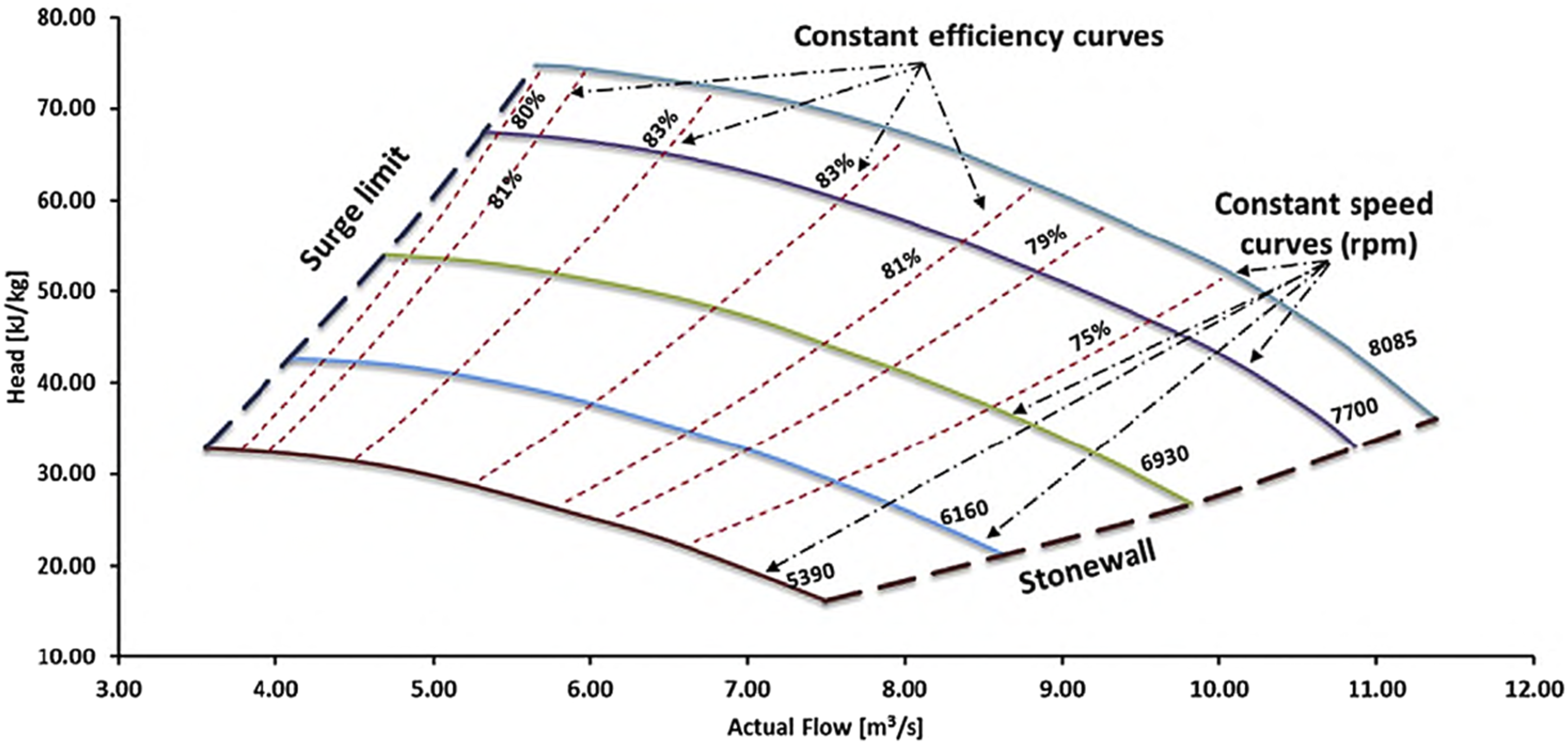
The operating point of the gas compressor is defined by the compressor map, the driver power, and the head-flow characteristics.35,44–46 The performance map is created based on compressor selection and from performance analysis. Thereafter, this is utilised to determine its operating conditions by evaluating its head-flow characteristics. Centrifugal compressor performance is a function of inlet volume flow rate, speed, isentropic head, isentropic efficiency,47,48 and compressor power requirement. The interrelationships among these parameters are shown in performance maps. The original equipment manufacturer can supply the compressor’s power requirement, efficiency, and speed after the performance analysis. The compressor’s drivers are sized based on the above information and the prevailing ambient conditions. The compressor operating speed is usually varied to control the flow through it. The parameters that affect the centrifugal compressor’s operating range are surge flow, choke, driver power, and maximum and minimum speeds. The performance curve of a turbo-compressor at constant wheel revolutions is restricted at both the low and high flow rates by the surge and stonewall points. Compressor surge is characterised by periodic gas flow in the compressor and the connected piping system. During part of the cycle, there is a backward flow. Surge flow occurs when the compressor operates at a lower flow rate, resulting in flow reversal and fluctuating bearing loads.42,49–56 It is an unstable condition, causing pressure oscillation that results in compressor damage, including the connected piping system.57–61 Control systems are designed to detect and prevent surges. This protects the compressor from damage. They must keep the compressor’s operating point within its safe operating range. This is done to avoid instabilities that cause breakdowns and engine downtime.
39
The Stonewall line is a phenomenon that occurs when the gas compressor speed reaches the speed of sound. This produces shockwaves that cause vibration in the parts.62,63 When the machine is operating at the stonewall point, the flow in the blade systems (wheel and bladed diffuser) is choked by shock waves. The flow can be unsteady. The acceptable operating range will be the enclosed area on the performance map. This takes into account safety, stability, and the anti-surge protection line. Figure 3 shows a typical centrifugal compressor map. Centrifugal compressor map.
64
Meira et al. 62 have proposed a new approach to performance modelling of compressor maps for natural gas pipelines. This work builds on the National Aeronautics and Space Administration’s loss theory to estimate energy losses. This includes accurately deriving the compressor characteristic curves, as well as the surge and choke lines. The results highlight the advantages of this modelling approach over conventional models. Thus, demonstrating its crucial role in reducing the operational costs of compressor stations. The reliability and validity of off-design simulations depend on performance maps. This should be assessed using available data, provided the engine’s design-point information is known.65–70 Therefore, the efficient operation of the compressor station and pipeline systems will depend significantly on the gas compressor performance maps, which are influenced by ambient conditions at the compressor station along the pipeline route. Several authors have investigated the performance of pipelines and gas compressors, accounting for ambient conditions. Albusaidi and Pilidis present an iterative method to determine the equivalent performance of centrifugal compressors under various operating conditions.71,72 This method accounts for changes in gas properties and stage efficiency, making it appropriate for hydrocarbon fuels. It was used to evaluate the performance of two multistage centrifugal compressors and compare their characteristics with measured data. The results demonstrated a strong agreement with the original values. Osiadacz and Chaczykowski compared isothermal and non-isothermal models of gas flow in pipelines. 73 The analysis revealed significant differences in pressure profiles along the gas pipeline.74,75 Sanaye and Mahmoudimehr have conducted both isothermal and non-isothermal modelling of a gas pipeline, accounting for ground temperature effects. 75 They derived a new form of conservation equations for compressible flow. 76 The results indicate a maximum difference of approximately 33.7% in the compressor head and 16.6% in rotational speed. This is based on established natural gas properties at various points along the pipeline. Lopez-Benito et al. 77 developed a numerical method to integrate a mathematical model that describes the flow in a natural gas pipeline under non-isothermal steady-state conditions. They transformed the model equations into a system of three explicit expressions for the spatial derivatives of the gas velocity, temperature, and pressure. This proposed method enables the prediction of gas pressure, temperature, and velocity at any point along the pipeline. However, these studies did not estimate the power requirements for gas compressors using the TERA approach. More so, these studies did not simultaneously account for isothermal, intermediate, and non-isothermal gas flow in pipelines. Additionally, they did not evaluate the performance maps of gas compressors under both design and off-design conditions, accounting for variations in gas flow temperature to assess the performance of both the gas compressor and the pipeline system.
Recent developments in the field have increasingly focused on thermodynamic optimisation and real-time monitoring of compressor station performance. Yang and Xuejiang. 78 applied Modular Dynamic System Greitzer (MDSG) compressor digital twin modelling and Short-Time Fourier Transform, Convolutional neural network (STFT-CNN) algorithm for recognising the surge case of series compressor systems. The average errors in the inlet and outlet pressures of a real suction compressor system are 1.88% and 0.67%, respectively. The accuracies of the training and test sets of the STFT-CNN method for compressor anomaly monitoring are 99.58% and 98.75%, respectively. Their results demonstrated that a digital twin model integrated with a condition-monitoring network can enable real-time simulation and monitoring of the compressor system. Similarly, Kai et al. 79 proposed a digital twin-driven intelligent control of a natural gas flowmeter calibration station to improve the efficiency of flowmeter calibration. The results show that the proposed method can accurately obtain the hydraulic state and control strategy and considerably enhance the calibration efficiency. Recent studies have proposed various machine learning-enhanced thermodynamic models for centrifugal compressor performance prediction, including Whale Optimisation Algorithm back-propagation neural network (WOA-BPNN), 80 similarity- and scaling-laws-informed neural networks (SINN). 81 The prediction accuracy of the proposed models is found to be better than conventional methods. Furthermore, Ojo et al. 14 conducted a techno-economic optimisation of the compressor station and pipeline segments for the proposed Trans-Saharan Gas Pipeline (TSGP) project under variable ambient conditions. The 4180 km pipeline would carry natural gas from Nigeria to Algeria’s export terminal on the Mediterranean Sea and eventually supply Europe. The optimisation problems were formulated to minimise lifecycle cost, with the location of the compressor stations as the decision variable. The results showed 12 compressor station locations along the pipeline route in one of the optimised cases. The optimised lifecycle cost is reduced by 12.95% compared to the baseline case. The optimised compressor station locations were at 1, 38, 76, 113, 150, 186, 222, 260, 296, 332, 368, and 408 segments of the pipeline. While these studies have advanced the state of the art, none have simultaneously evaluated all three thermal flow regimes (isothermal, intermediate, and non-isothermal) within a unified TERA framework that links pipeline hydraulics, compressor performance maps, and economic analysis, as is done in the present study.
Therefore, the objective of this study is to determine the power requirements of compressor stations under different gas-flow temperature conditions. This analysis is based on three flow assumptions: isothermal, intermediate, and non-isothermal. The study utilises the techno-economic and environmental risk analysis (TERA) framework to guide the evaluation of natural gas flow in pipelines. This study presents the following information for the first time: • What gas compressor sizes are needed for different flow conditions at each compressor station location, considering isothermal, intermediate, and non-isothermal gas flow temperature assumptions based on the TERA approach? • What are the effects of gas compressor powers at isothermal, intermediate, and non-isothermal gas flow temperature conditions? • What are the impacts of gas compressor operating points at varying flow conditions? • How do we select appropriate gas compressors based on the analysis?
The remainder of this paper is organised as follows. The Methodology presents and describes the modules that comprise the TERA framework. Gas compressor powers were evaluated under varying flow conditions, and performance maps were generated using scaling analysis. The essential outcome of the study is presented in the results and discussion section. Subsequently, the study's conclusion and limitations are highlighted, and directions for future research are suggested.
Methodology
This study employs an integrated analytical approach to assess the power requirements of compressor stations under varying thermal flow regimes. The core of the methodology is the Techno-economic and Environmental Risk Analysis (TERA) framework, implemented in MATLAB environment, which synthesises pipeline hydraulics, gas thermodynamics, and compressor performance. The overarching process, visualised in the flowchart in Figure 4, is summarised as follows: • • • • • Flowchart of the Techno-Economic and Environmental Risk Analysis (TERA) framework used in the present study. The integrated model processes input parameters through sequential pipeline and compressor modules, conditioned by the ambient data, to produce technical and economic outputs for compressor selection. Pipeline elevation-distance profile.
82
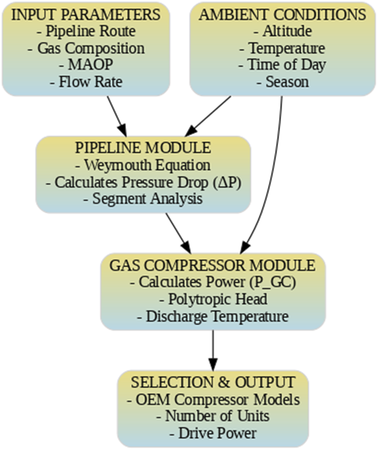
The subsequent sections detail the assumptions, environmental data, and specific mathematical models that underlie this framework.
Environmental conditions
The altitude and ambient conditions at the compressor station along the pipeline route will significantly affect the gas compressor’s performance. The altitude at which the compressor station and pipeline operate will affect the gas compressor’s performance because altitude significantly affects ambient temperature. Therefore, ambient temperature and altitude at the location should be considered when assessing the gas compressor performance. The average daily ambient temperature for the location where the compressor station would be installed was obtained from the Trans-Saharan Gas Pipeline report.
27
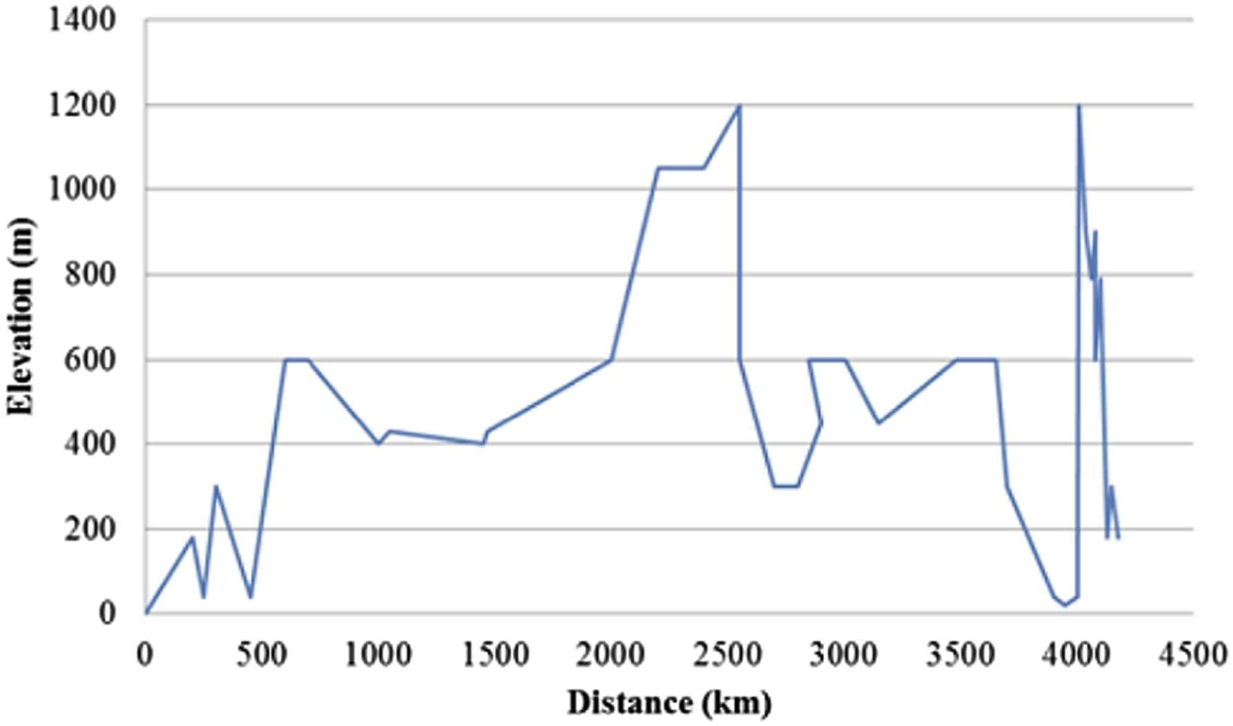
The elevation-distance profile was retrieved from Ref. 82. Figure 5 shows the pipeline elevation-distance profile utilised in this study.
82
Figure 6 illustrates the cumulative three-hourly variation in ambient temperature during one season of the year, relating to the time of day at the compressor stations along the pipeline route. This study uses the average temperature for each season, assuming 4 months per season. Ambient temperatures recorded at various stations during the winter season.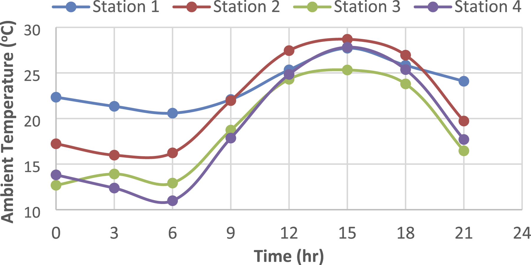
The ambient conditions form the basis for analysing the pipeline and gas compressor models in this study. These operating conditions have a significant impact on the techno-economics of the proposed Trans-Saharan Gas Pipeline project.
Pipeline and gas compressor model assumptions
The following shows the assumptions utilised in the analysis of the pipeline and gas compressor models: 1. Constant pipe diameter for the whole pipeline length. 2. Constant natural gas composition. 3. The gas flow temperature is assumed to be equal to the location’s ambient temperature at the compressor station’s suction or discharge point.
83
4. Baseline case comprises 18 compressor stations in a predetermined location. 5. The pipeline is clean. 6. The operation of the gas compressors is based on the variation in the station location ambient temperatures at varying gas flow temperature conditions. 7. The selected gas compressors are expected to operate over the project lifecycle.
The limitations introduced by assuming constant pipe diameter, constant gas composition, clean pipeline conditions, and steady-state thermal behaviour are that, with a constant pipe diameter, variations in flow conditions are mostly influenced by temperature and pressure changes along the pipeline. A constant gas composition is valid for steady-state thermal analysis. A steady state thermal treatment ignores the transient and therefore limits full compressor analysis, while clean pipeline conditions provide no information about degradation over the project lifecycle.
Gas properties calculation and pipeline pressure drop
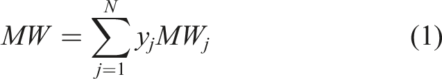
The natural gas molecular weight is estimated using a weighted average method from the known component’s gas properties as follows:
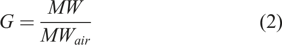
The natural gas gravity
The ideal gas equation of state is modified to the real gas equation of state by considering compressibility effects, as natural gas pipelines often operate at higher pressures. The real gas equation of state can be expressed as:

The compressibility factor
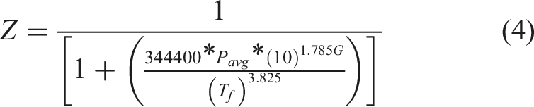
The average pressure is used to calculate the compressibility factor of natural gas at the flowing temperature. The equation for the compressibility factor is applicable when the average gas pressure exceeds 690 kPa; Otherwise, a value of one is assumed.
The Weymouth equation is used for pipelines that transport natural gas over long distances, with high gas throughput and pressure, and with large diameters.4,27,84 It calculates the natural gas flow rate at a given pressure without using a friction factor. Instead, it accounts for the pipe’s internal conditions using a pipeline efficiency factor. Thus, ensuring accurate evaluation of pressure drop over other methods, such as the classical Darcy-Weisbach method.
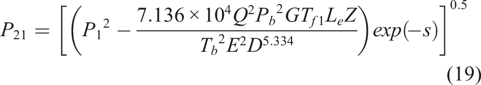
For a given pipe inlet pressure
The equivalent length
The elevation adjustment parameter
Hence, the pressure drop along the natural gas transmission pipeline segment is the algebraic difference between the estimated outlet pressure of the pipe and the known inlet pressure defined by:

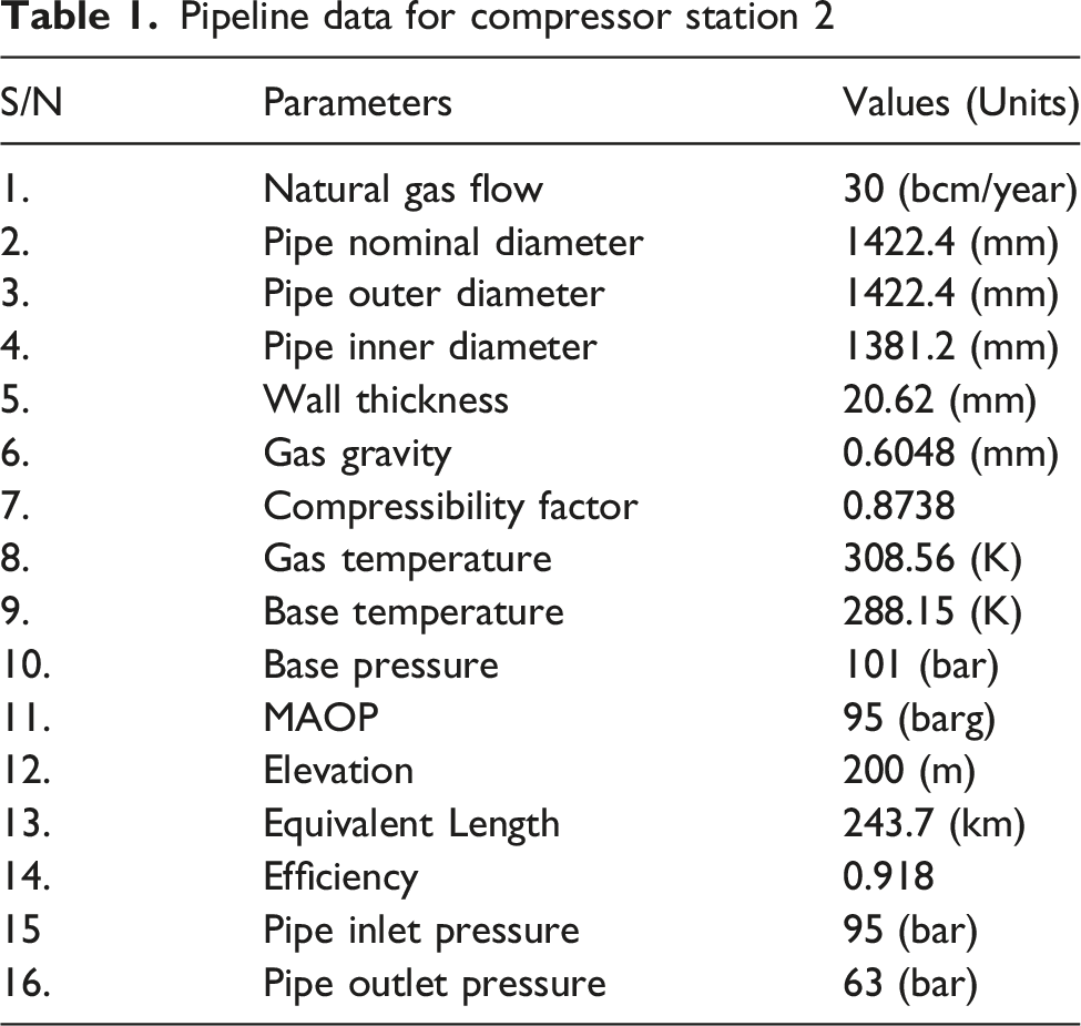
Pipeline data for compressor station 2
Gas compressor model
The compression ratio of the gas compressor at each station is evaluated as follows: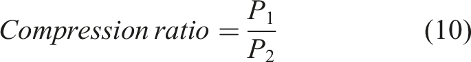
The discharge temperature of the gas compressor for a polytropic process depends on the gas compressor inlet temperature, compression ratio, polytropic exponent and the compressibility factors and is defined by: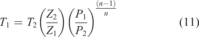
The gas compressor discharge temperature can strain the compressor components and reduce its reliability. Therefore, it is crucial to regulate this temperature by adequate cooling or maintaining it within an acceptable range. Liu et al.
85
have investigated a three-dimensional simplified model of an air cooler for a natural gas compressor station. This model is used to simulate and study the cooling effect of a finned-tube dry air cooler on high-temperature, high-pressure natural gas at the compressor outlet. The polytropic head generated by the gas compressor represents the amount of energy delivered to the natural gas per unit mass.
86
It depends on the inlet temperature, molecular weight, compression ratio, compressibility factor, and polytropic exponent. It is defined by: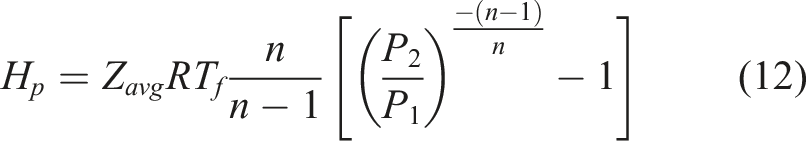
The gas compressor power requirement can be written as: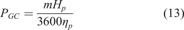
The polytropic efficiency 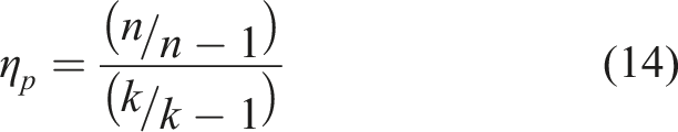
The gas compressor’s actual volume flow rate at suction conditions 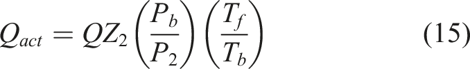
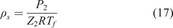
The gas compressor’s actual mass flow rate 
Changes in gas flow temperature will affect the actual volumetric flow rate. This is because the gas compressor’s suction conditions depend on pressure and temperature.
Gas compressor power evaluation at varying flow conditions
The effect of gas compressor powers at varying gas flow temperature conditions was evaluated in this study. This is based on three scenarios that assume the gas flow temperature matches the location’s ambient temperature at the gas compressor station’s suction or discharge point.
83
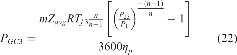
The scenarios are described as follows: 1. Scenario 1 depicts the isothermal gas flow temperature condition. This condition assumes a constant gas-flow temperature of 22°C at all times of the day and in all seasons of the year. 2. Scenario 2 depicts the non-isothermal gas flow temperature condition. This condition assumes that the prevailing location time-based ambient temperature is equivalent to the gas-flow temperature. This depends on the ambient temperature variation across the three seasons: winter, dry, and hot. A change in the ambient temperature at the gas compressor station location leads to an equivalent change in the gas flow temperature at the reference time. 3. Scenario 3 depicts the intermediate gas flow temperature condition. This scenario assumes a constant average value for the isothermal and non-isothermal gas flow conditions described above. This value remains constant, as in scenario 1, for all times of the day and throughout all seasons of the year. However, they depend on the prevailing time-based non-isothermal ambient temperature at each gas compressor station.
Distance, elevation, and ambient temperatures recorded at various stations.
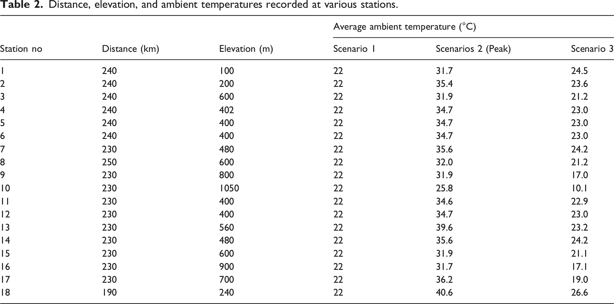
The pipeline inlet pressure is 9500 kPa. The operational constraint is the pipeline’s maximum allowable operating pressure of 9500 kPa. Furthermore, all gas compressors installed at each compressor station along the pipeline route are expected to have a pressure ratio between 1.40 and 1.66, as suggested by the Trans-Saharan Gas pipeline report. 27 The three scenarios described the different operating conditions of the gas compressor. The basis for the isothermal modelling assumption (Scenario 1) is that transmission pipelines at gas compressor stations may be insulated, adiabatic, and installed at locations where heat exchange between the gas and its surroundings is sufficient to maintain a constant temperature. This is most applicable to buried pipelines, which are installed below ground level, where the ground temperature exerts a dominant thermal influence, causing the gas temperature to approach it with little or no change. An insulated pipeline is integrated with insulating material to regulate gas temperature and prevent heat losses. Therefore, the assumption of an isothermal model is justified as one of the scenarios considered in this study. However, in real life, ambient temperature varies with the time of day and the season. Pipelines with above-ground segments are usually installed partially or entirely above the ground surface, exposing them to ambient conditions. For the long-distance Trans-Saharan Gas Pipeline route considered in this study, with above-ground sections exposed to diurnal ambient variation, this isothermal modelling assumption is expected to introduce a systematic deviation in compressor power of approximately 2–5% relative to the non-isothermal case. It is important to note that insulation can be applied to either buried or above-ground pipelines. The intermediate thermal model (Scenario 3) assumes a constant average value between the isothermal and non-isothermal models. The intermediate assumption uses a time-averaged temperature that captures mean seasonal conditions; it reduces the error relative to the isothermal case but still underestimates peak power demand by approximately 1–3%. The non-isothermal assumption (Scenario 2), which directly equates gas flow temperature to the local time-varying ambient temperature, represents the most physically realistic scenario for above-ground and surface-laid segments and introduces no systematic bias relative to real-world ambient-driven operation; its residual uncertainty arises primarily from the accuracy of the input ambient temperature data (±0.5–1°C typical for meteorological records), leading to an estimated power uncertainty of less than ±0.5%. All three assumptions are valid for steady-state, fully developed flow in single-phase dry natural gas pipelines operating within the pressure range of 60–100 bar considered in this study. These conditions are expected in the oil and gas industry, which deals with long-distance transmission pipelines. Consequently, they show the full range of temperatures experienced at the gas compressor stations and along the pipeline routes.
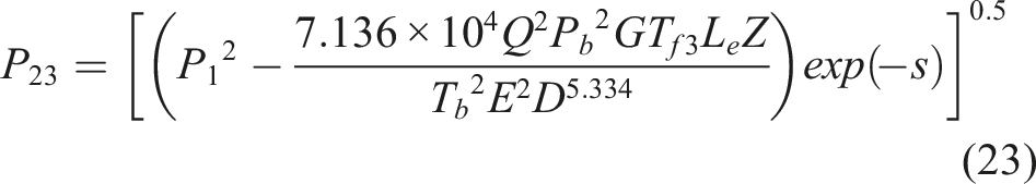
By combining equations (12) and (13), the gas compressor powers based on the three scenarios are defined as follows: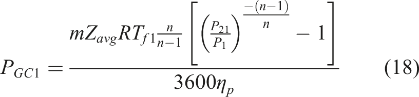


Gas compressor performance map
The performance maps of gas compressors illustrate how power, polytropic head, pressure ratio, efficiency, and discharge temperature vary with actual volume flow rates at different speeds. The gas compressor performance maps were generated from scaling analyses of the original equipment manufacturer’s maps. The steps utilised in obtaining the corrected volume flow rate for the new maps are outlined below: i. Obtain the actual volume flow at the design point from the original equipment manufacturer’s map ii. Correct this flow iii. Obtain the actual volume flow at the design point for the new map iv. Correct this flow v. Obtain the scaling factor for the corrected volume flows vi. Obtain the actual volume flow at off-design conditions from the original equipment manufacturer’s map vii. Correct these flows viii. Obtain the corrected volume flow at off-design conditions for the new map using the scaling factor obtained in item v ix. Obtain the actual volume flow for these corrected flows for the new map
The corrected mass flow rate 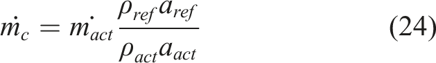
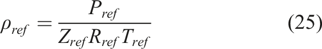
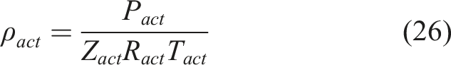


Substituting the corrected mass flow rate with the corrected volume flow rate, noting that the gas compressor under study is a constant-diameter machine. The simplified form of the corrected volume flow rate is obtained by substituting equations (25)–(28) into equation (24):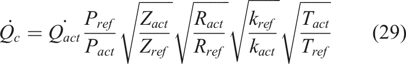
The actual volume flow for the new compressor map was obtained using equation (29) and the scaling factor for the corrected volume flow rate defined by: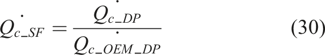
The following shows the steps utilised in obtaining the pressure ratio curves for the new maps: i. Obtain the pressure ratio at the design point for the new map ii. Obtain the pressure ratio at the design point from the original equipment manufacturer’s map iii. Obtain the scaling factor for the pressure ratio at the design point iv. Generate pressure ratio data at off-design conditions from the original equipment manufacturer map v. Compute the equivalent pressure ratio at off-design conditions for the new map using the scaling factor obtained from item iii
New gas compressor maps for the pressure ratio were obtained by a scaling factor defined by: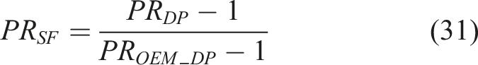
The steps utilised in obtaining the polytropic efficiency, polytropic head and discharge temperature curves for the new maps are as follows: i. Obtain the polytropic efficiency, polytropic head and discharge temperature at the design point for the new maps ii. Obtain the polytropic efficiency, polytropic head and discharge temperature at the design point from the original equipment manufacturer maps iii. Obtain the scaling factors for the polytropic efficiency, polytropic head and discharge temperature at the design point iv. Generate polytropic efficiency, polytropic head and discharge temperature data at off-design conditions from the original equipment manufacturer maps v. Compute the equivalent polytropic efficiency, polytropic head and discharge temperature at off-design conditions for the new maps using the scaling factor obtained from item iii
New compressor maps were obtained for the compressor polytropic efficiency, polytropic head and discharge temperature by defining their scaling factors as follows: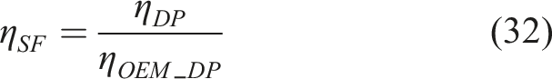
The following section presents and discusses the results of the TERA framework method utilised in this study.
Results and discussion
Figure 7 illustrates the pressure gradient of the pipeline at the location of Compressor Station 3. Pressure drops along the pipeline for compressor station 3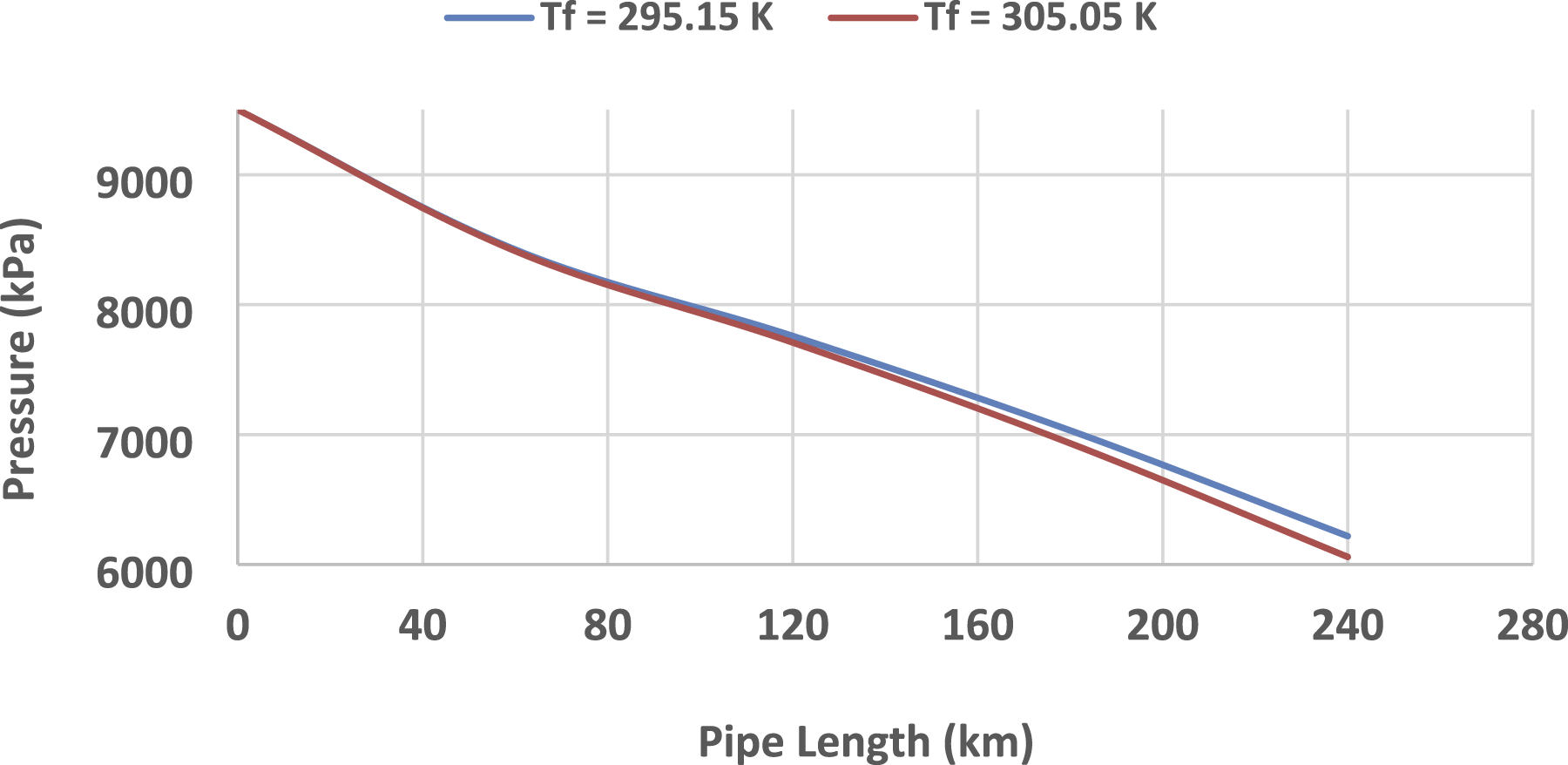
The pipeline inlet pressure is 9500 kPa. The pressure drops at compressor station 3 vary with pipe distance and gas flow temperature, as described in scenarios 1, 2, and 3. The pressure drop increases with pipe length until it reaches its maximum at 240 km. This is at isothermal and intermediate temperatures of 295.15 K and 305.05 K, depicted by scenarios 1 and 3, respectively. These maximum pressure drops are equivalent to the low pipe-discharge pressures observed at compressor station 3. Considering the non-isothermal condition with a variation in gas flowing temperature, as described by scenario 2. A rise in the gas flow temperature from 295.15 K to 305.05 K at a pipe length of 240 km leads to an increase in the pressure drop. Similarly, a decrease in gas temperature causes lower pressure drops in the pipeline.
The pressure drop variation along the pipeline length at maximum gas-flow temperatures is illustrated in Figure 8 for each compressor station. Pipeline pressure drops at various compressor station locations.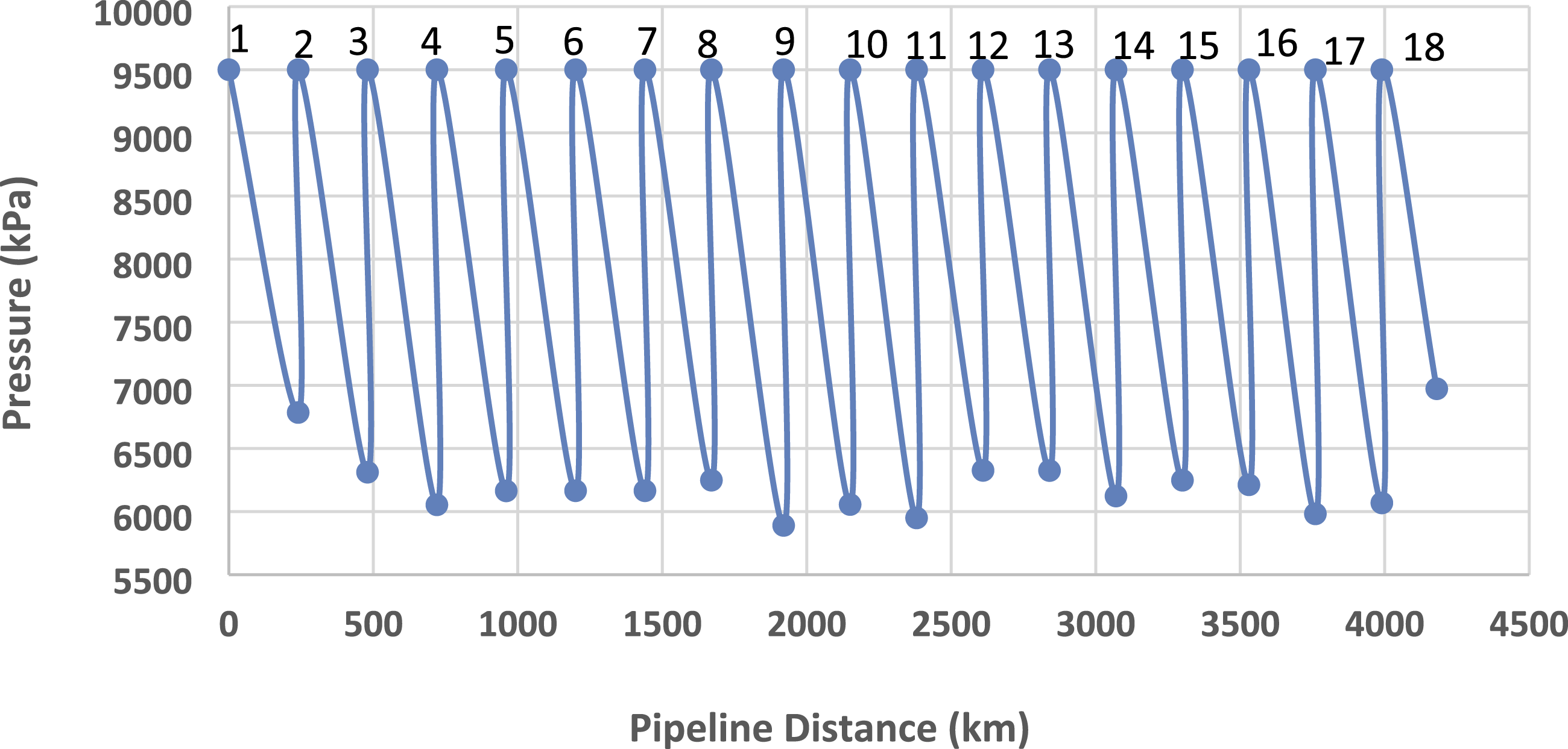
The pressure drops to 6785 kPa and 6312 kPa at compressor stations 2 and 3, respectively. Thus, gas compressors are required at these locations to increase the low pressures to the pipeline operating pressures of 9500 kPa. This ensures a continuous supply of natural gas through the pipelines.
Effects of gas compressor suction pressure
Figure 9 displays the gas compressor suction pressure at each compressor station along the pipeline route for scenarios 1 and 3. The suction pressure varies from one station to another. Gas compressor suction pressure for Scenarios 1 and 3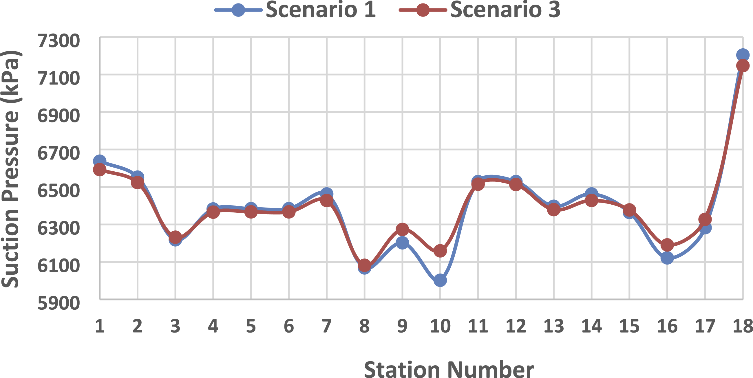
Compressor stations 10 in scenario 1 and 8 in scenario 3 have the lowest suction pressures. This is because these station locations are associated with the lowest average pipeline pressure. Therefore, high gas compressor power requirements are needed at these locations. Conversely, compressor station 18 has the highest gas-compressor suction pressure in scenarios 1 and 3. This is because this station location is associated with the highest average pipeline pressure. Hence, low gas compressor power are needed at these locations.
Figure 10 shows the gas compressor suction pressures for the winter season at stations 1–4 under non-isothermal gas-flow temperature conditions for scenario 2. Gas compressor suction pressures for Scenario 2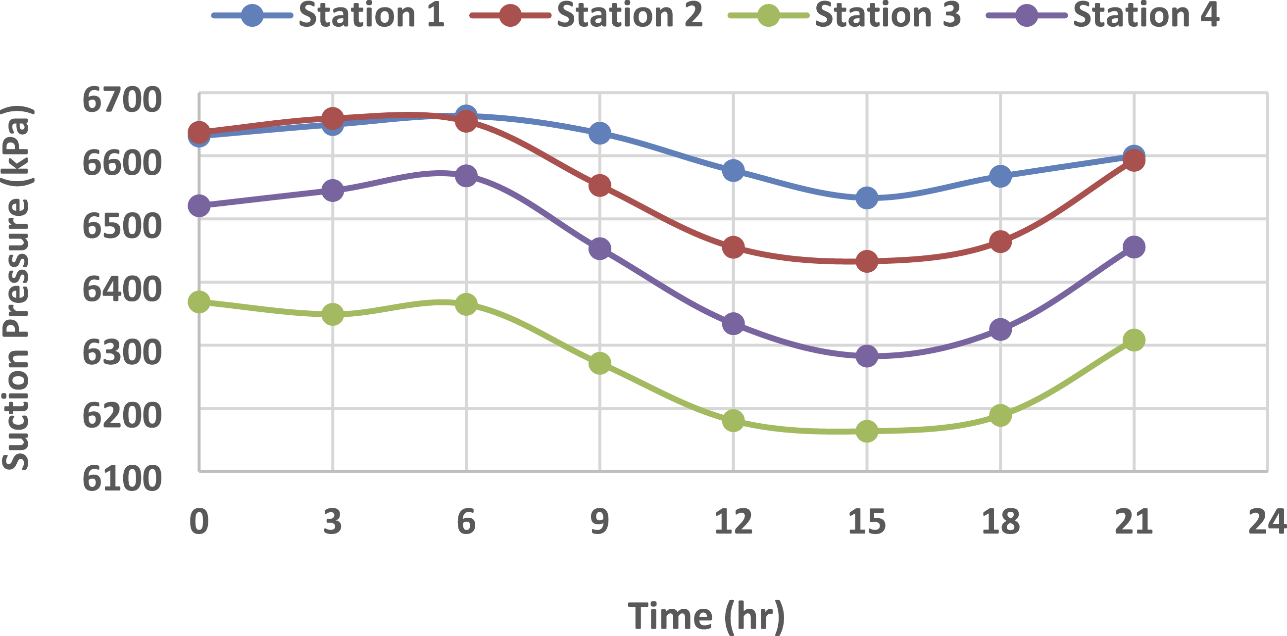
The gas compressor suction pressures are lowest at 15:00 hours, when the ambient temperature is highest. Furthermore, the average pipeline pressure is lowest at this time of day. Therefore, high power is required for the gas compressor. Conversely, the suction pressures are highest at 06:00 hours, when the ambient temperature is lowest. More so, the average pipeline pressure is highest at this time of day. Consequently, low gas-compressor power is required. Furthermore, the results show that for every 1% increase in ambient temperature, the gas compressor suction pressure decreases by an average 0.1%. This finding is valid across the full range of ambient temperatures considered in this study, provided other conditions remain constant.
Therefore, the results indicate that the gas compressor suction pressure depends on pipe distance, elevation, and ambient temperature.
Gas compressor pressure ratio at different stations
The gas compressor pressure ratio, also known as the compression ratio, is defined as the ratio of its discharge pressure to its suction pressure. In this study, the maximum allowable operating pressure (MAOP) of the pipeline is set at 9500 kPa, which corresponds to the discharge pressure of the gas compressor.
Figure 11 displays the compressor pressure ratio at each station along the pipeline route for scenarios 1 and 3. Gas compressor pressure ratio for Scenarios 1 and 3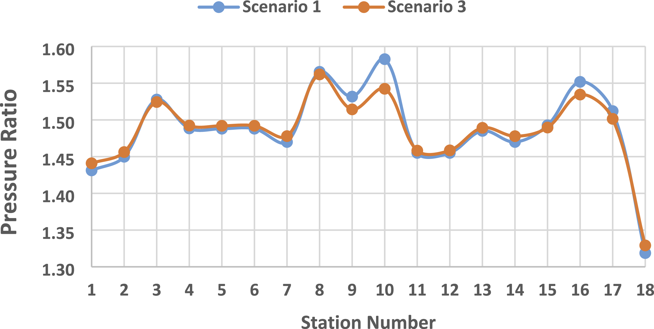
Compressor station 18 has the lowest pressure ratio for scenarios 1 and 3, as shown in Figure 11. Therefore, this station location will require the lowest power from the gas compressor. Conversely, stations 10 and 8 in scenarios 1 and 3, respectively, have the highest gas compressor pressure ratios. Therefore, these station locations will require the highest compressor power.
Figure 12 shows the gas compressor pressure ratios for the winter season at stations 1 to 4, under non-isothermal gas flow temperature conditions for scenario 2. The highest compressor pressure ratios at 15:00 hours will require the highest compressor power. However, the lowest pressure ratios experienced at 06:00 hours will require the lowest compressor power. Gas compressor pressure ratio for Scenario 2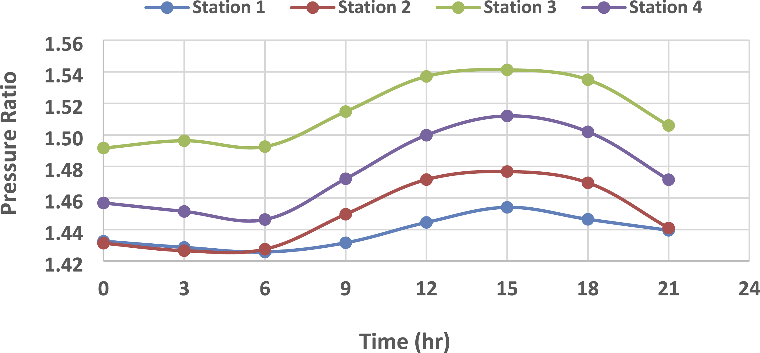
Gas compressor discharge temperature at different stations
The discharge temperature is the increase in gas temperature resulting from compression of natural gas. Figure 13 illustrates the gas compressor discharge temperature at each station along the pipeline route for scenarios 1 and 3. Gas compressor discharge temperature for Scenarios 1 and 3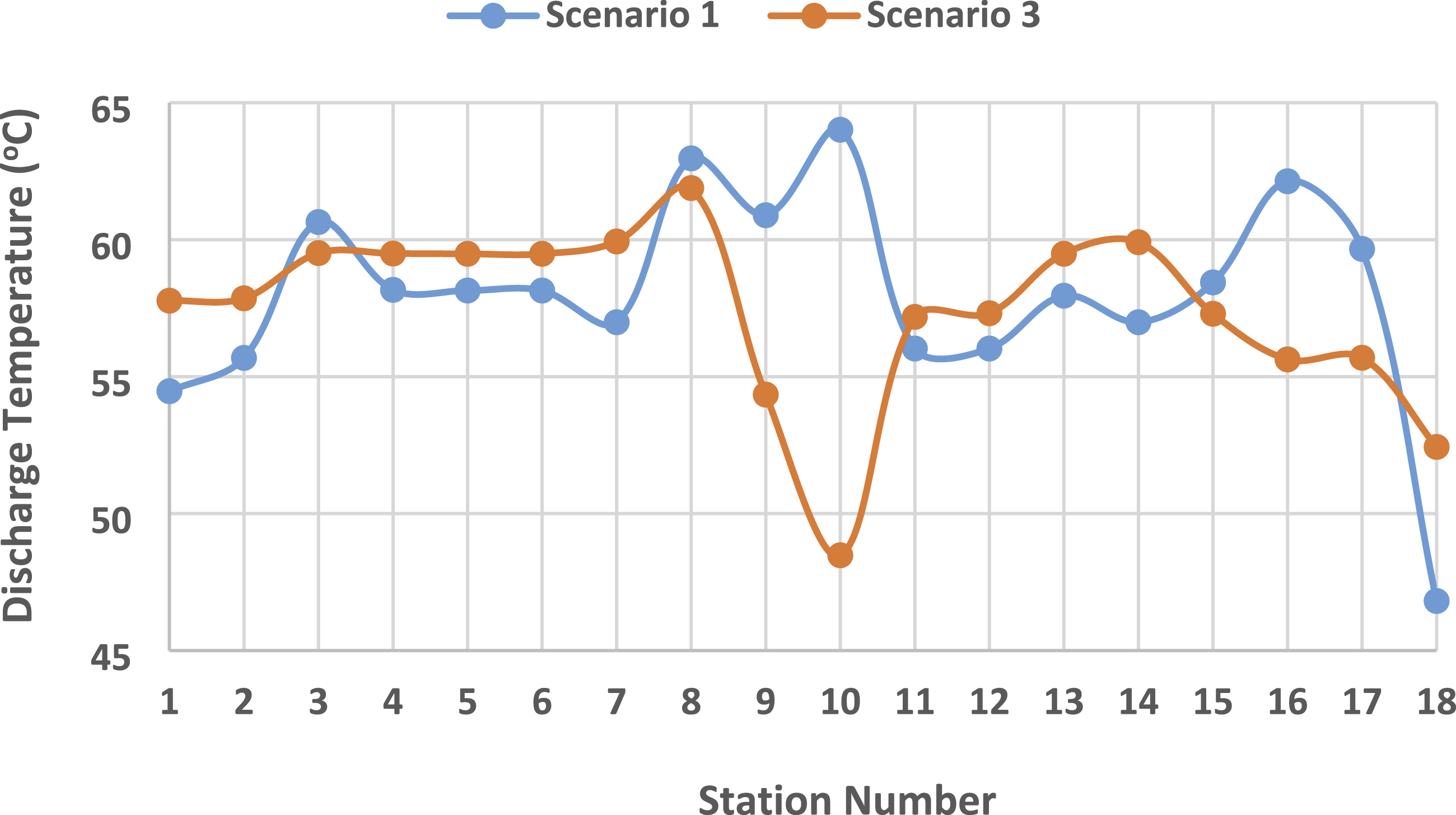
Compressor station 10, which has the highest pressure ratio in Figure 11 for scenario 1, also has the highest discharge temperature. Similarly, Compressor Station 8, which has the highest pressure ratio in Figure 11 for Scenario 3, also has the highest discharge temperature, as shown in Figure 13. Therefore, we conclude that the gas discharge temperature increases with the compression ratio. Thus, a higher gas compression ratio results in a higher discharge temperature of the compressed natural gas. However, compressor station location 10, with the second-highest gas compression ratio in Figure 11 for scenario 3, has the lowest discharge temperature as shown in Figure 13 for scenario 3. This observation is due to the high elevation at this compressor station and the lower suction intermediate temperature at this location compared to other compressor stations.
Figure 14 shows the gas compressor discharge temperature for the winter season at stations 1–4 under non-isothermal gas-flow conditions for scenario 2. The highest gas compressor discharge temperature occurs at 15:00 hours, when the gas compression ratio is at its highest. In contrast, the lowest discharge temperature occurs at 06:00 hours, when the gas compression ratio is at its lowest. Similar explanations can be given for other compressor station locations. Gas compressor discharge temperature for Scenario 2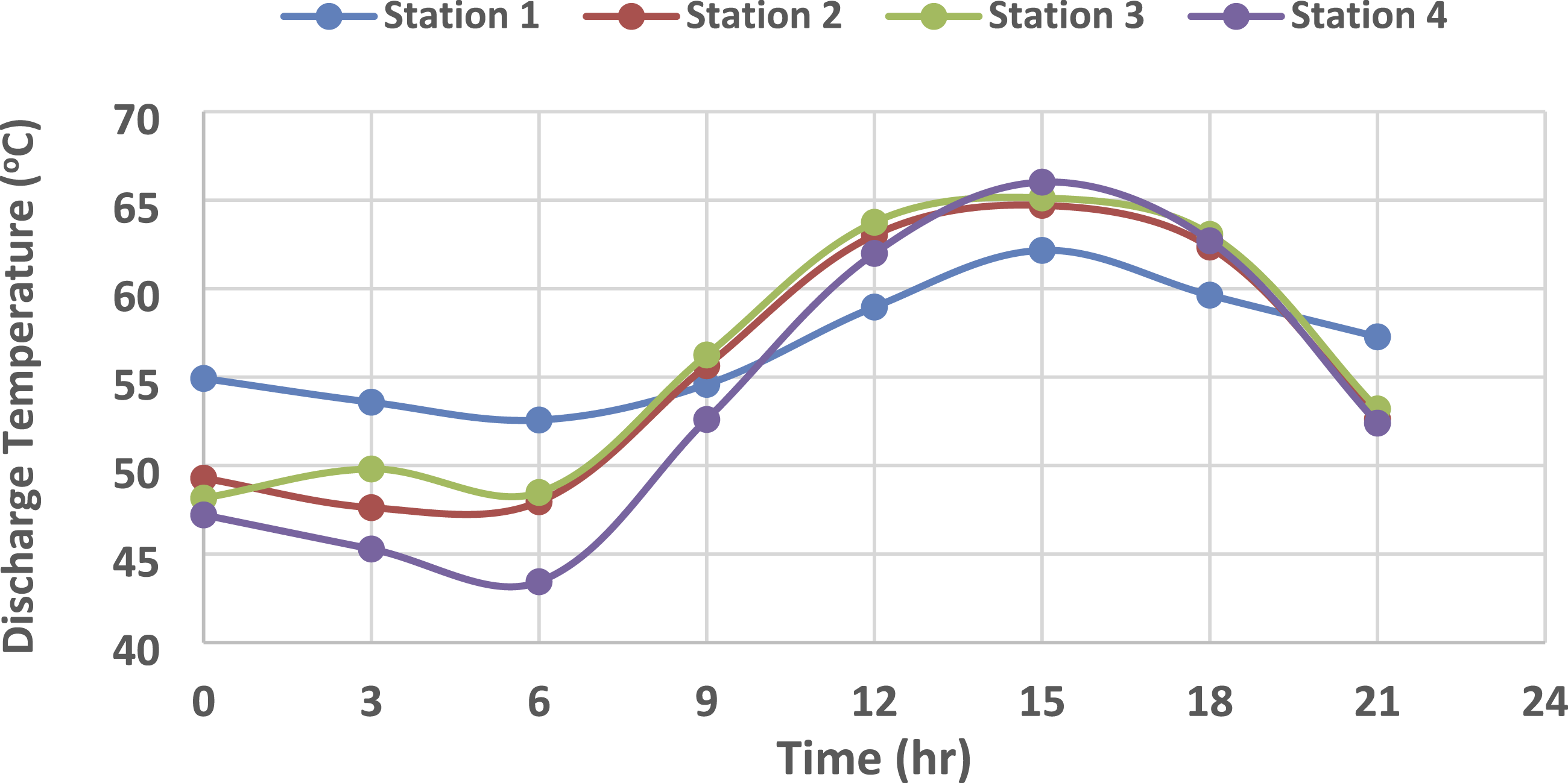
It is beneficial to control the gas compressor discharge temperature within specified limits to optimise gas transport through the pipelines. One way of achieving this is to install a cooling device at the gas compressor discharge point.
Gas compressor power at varying flow conditions at different stations
Figure 15 shows the gas compressor power requirements at each station along the pipeline route for scenarios 1 and 3. Considering scenario 1, compressor station 10 has the highest gas compression power among all stations. This station location is associated with the lowest gas compressor suction pressure, the lowest average pressure, and the highest gas compression ratio. The increase in pipeline distance and elevation results in a corresponding decrease in the gas compressor suction pressure. Therefore, this leads to an increase in the gas compression ratio, the polytropic head, and, thus, the gas compressor power requirement. Moreover, the lower gas compressor power requirement at compressor station 10 in scenario 3, compared to the exact location in scenario 1, is due to the lower suction intermediate temperature at this station. However, the lowest gas compressor power requirement for scenarios 1 and 3 occurs at compressor station 18. This location is associated with the highest gas compressor suction pressure, the highest pipeline average pressure, and the lowest gas compression ratio. Furthermore, gas compressor power decreases with increasing gas compressor suction pressure, due to a lower compression ratio and polytropic head. Gas compressor power requirement for Scenarios 1 and 3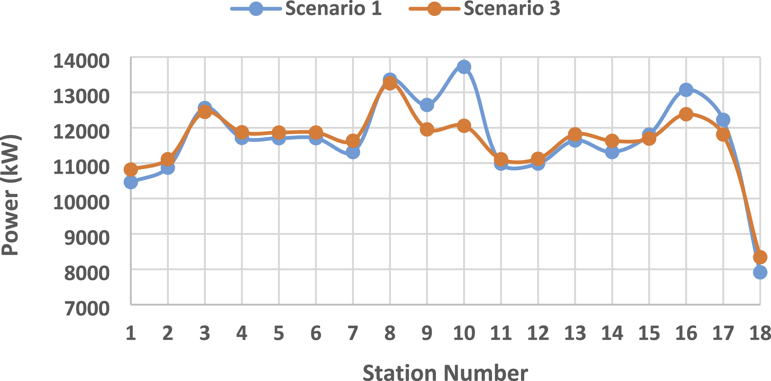
Similar explanations could be given for other compressor stations. Consequently, the results indicate that the gas compressor inlet temperature and the characteristics of the compressor station location significantly affect the gas compressor power requirements.
Figure 16 illustrates the gas compressor power requirement for the winter season at stations 1 to 4 under non-isothermal gas-flow temperature conditions for scenario 2. The characteristics of the compressor station location significantly impact the gas compressor’s power requirement. These location characteristics depend on the prevailing ambient temperature, the time of day, and the season. More so, since the pipe diameter, natural gas composition and flow rate are constant. The highest gas compressor power requirement occurs at 15:00 hours, when the ambient temperature is highest across all compressor stations. Conversely, the lowest gas compressor power requirement occurs at 06:00 hours, when the ambient temperature is lowest across all compressor stations. The variation in the gas compressor’s power requirement is due to changes in ambient temperature with time of day and station location characteristics. Additionally, the results show a 0.3% average increase in the power required by the gas compressor to move the gas for every 1% increase in ambient temperature, across the temperature ranges considered in this study, assuming all other conditions remain the same. Gas compressor power requirement for Scenario 2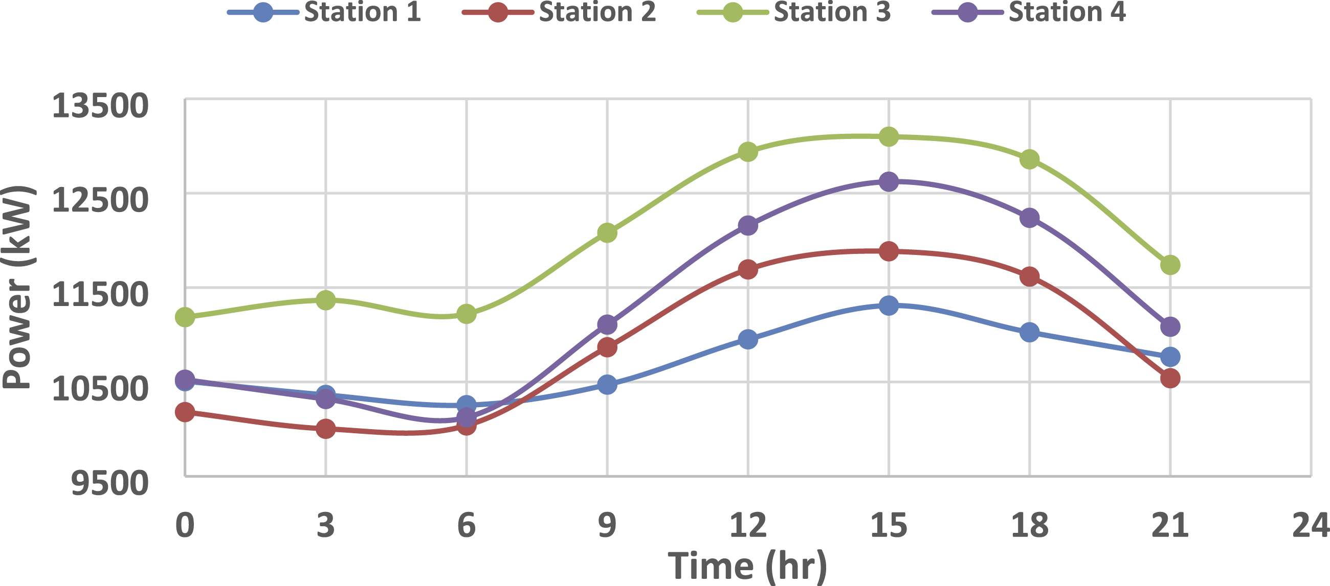
Comparison with Aspen HYSYS
Validation with aspen HYSYS.
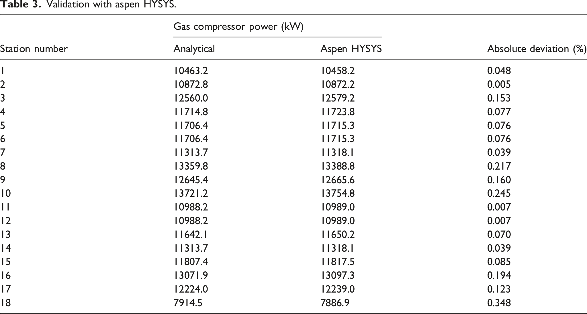
There is strong consistency between the analytical and simulation results from Aspen HYSYS. The maximum absolute percentage difference between the gas compressor powers occurs at compressor station 18, at about 0.348%. Nevertheless, this difference is negligible. Therefore, the analytical methods employed in this study can be applied in the natural gas pipeline industry.
To further characterise the accuracy of the analytical model, the mean absolute percentage deviation (MAPD) across all 18 stations is calculated as 0.035%, confirming that the analytical approach is robust and not merely accurate at isolated points. The relatively larger deviation at Station 18 (0.348%) is attributed to the combined effect of the lowest compression ratio and highest suction pressure at that location, where small absolute differences in thermodynamic property calculations are proportionally amplified. Importantly, 0.348% remains well below the ±1% tolerance commonly accepted in compressor performance analysis for engineering design purposes.
Measurement and modelling uncertainty analysis
A structured uncertainty analysis was conducted to assess the combined effect of instrument tolerance and modelling assumptions on the key output performance indicators. The primary sources of uncertainty in the present analytical framework are: (i) ambient temperature measurement, for which meteorological instruments typically carry a tolerance of ±0.5°C; (ii) pipeline inlet pressure specification, with a representative gauge-instrument tolerance of ±0.2%; (iii) compressibility factor
Error propagation through equations (12) and (13) was estimated using a first-order Taylor series expansion. The resulting combined uncertainty in the calculated compressor power
Having validated the gas compressor power demand against Aspen HYSYS and confirming strong consistency, the next section analyses the gas compressor performance map.
Gas compressor performance map
The variation of the gas compressor pressure ratio, polytropic head, and discharge temperature with the actual inlet volume flow is illustrated in Figures 17–19, respectively. They show the impact on gas compressor performance. Pressure ratio curve for station 3 Polytropic head curve for station 3 Discharge temperature curve for station 3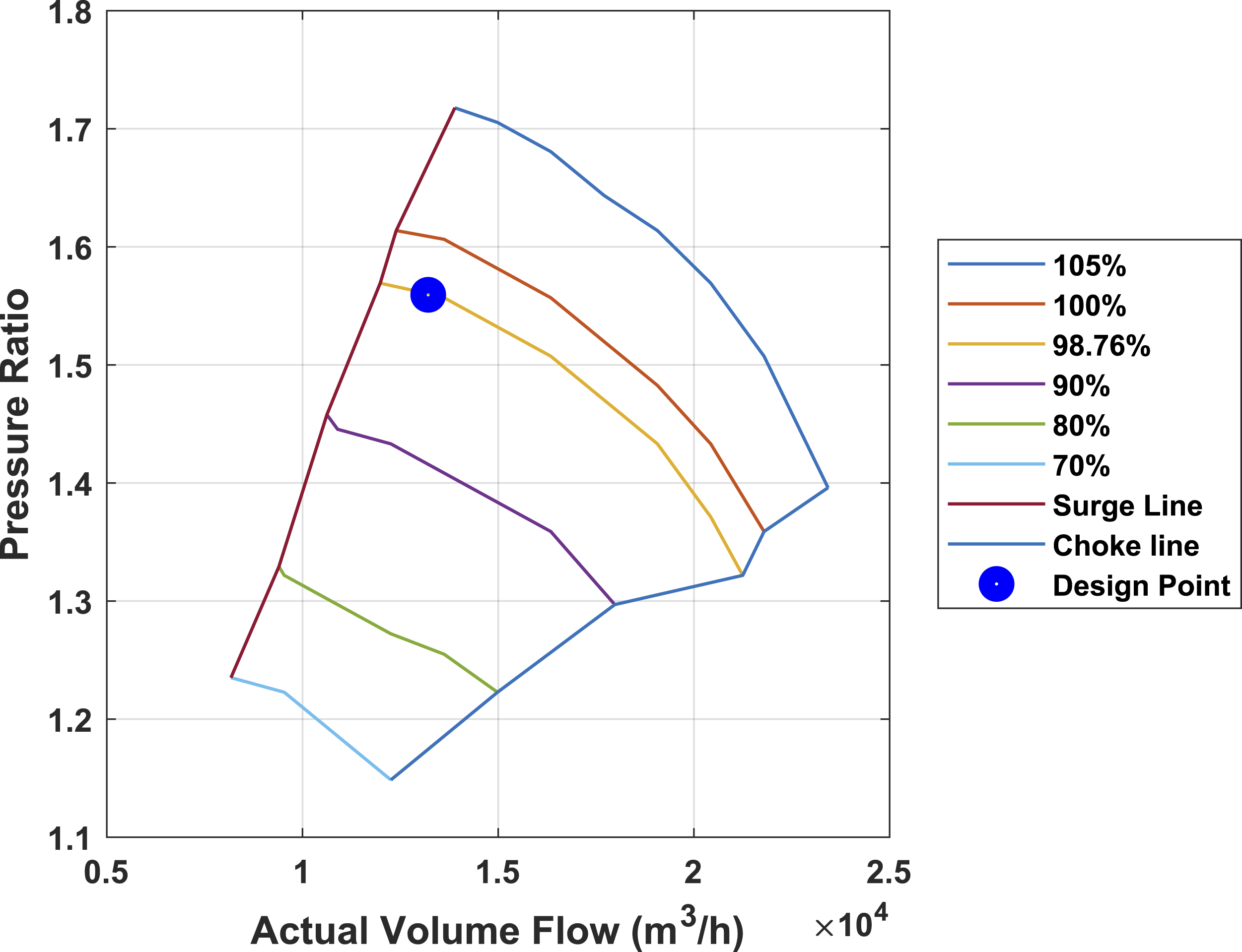
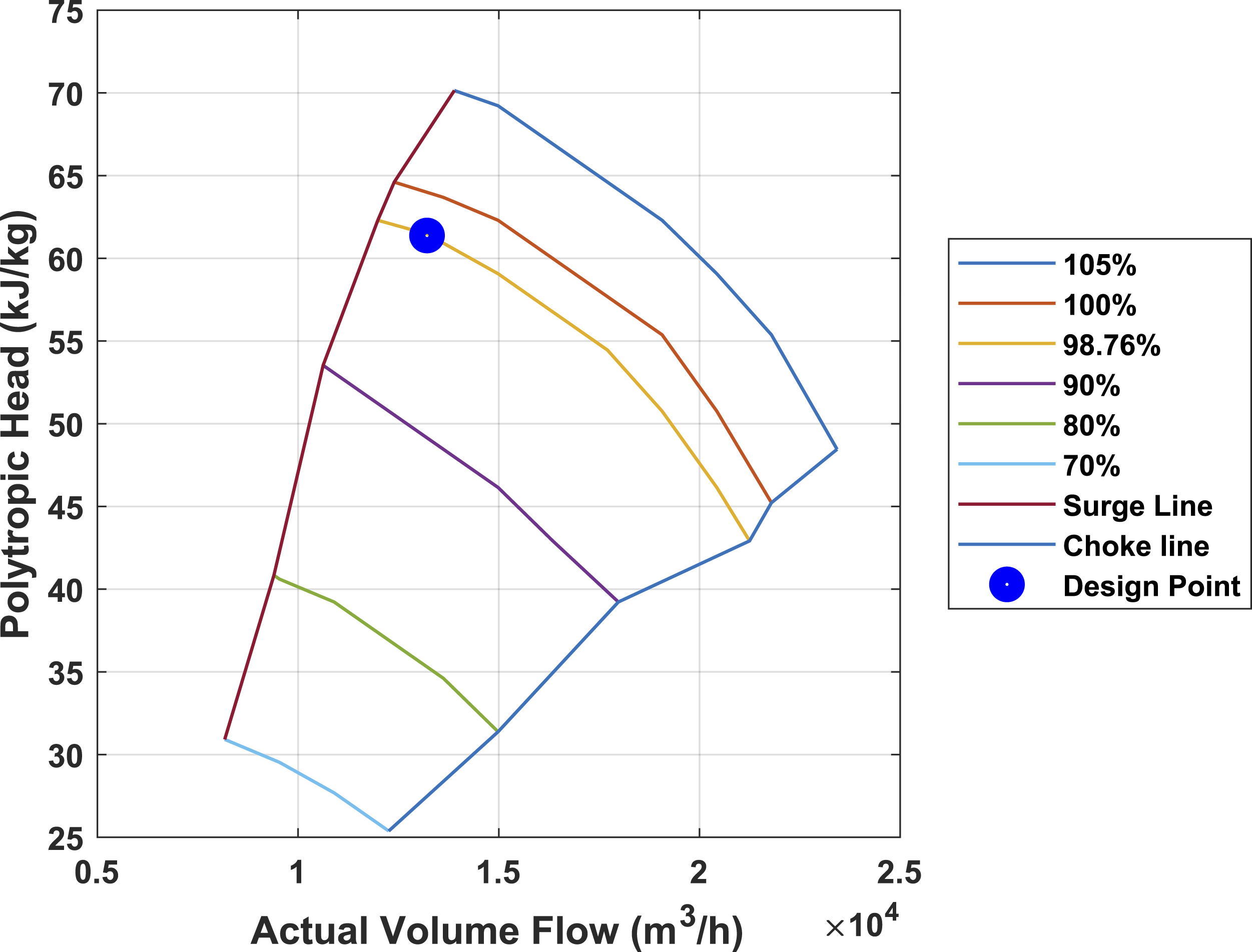
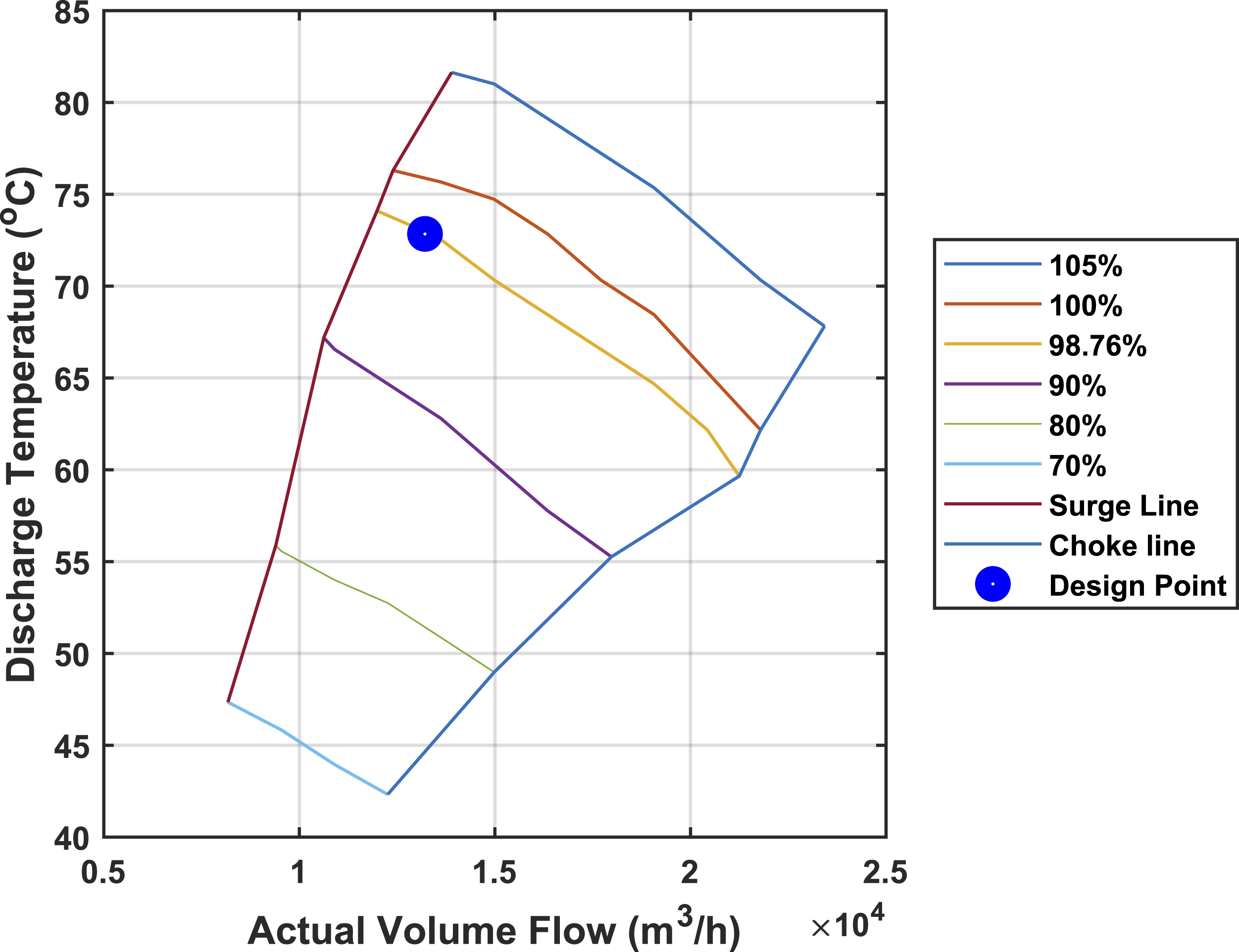
The results show increases in the gas compressor pressure ratio, polytropic head, discharge temperature, and actual inlet volumetric flow rate with increasing gas compressor shaft rotational speed. However, at a fixed gas compressor shaft rotational speed, the gas volumetric flow rate decreases as the suction pressure decreases, the polytropic head increases, and the gas compressor discharge temperature increases. The increase in the polytropic head is due to a reduction in the gas compressor suction pressure. Moreover, the surge margin increases with rising discharge temperature.
The performance maps above show the gas compressor surge line, the choke line, and the design point.
Figure 20 illustrates the variation in gas compressor polytropic efficiency with actual inlet volume flow at different rotational speeds on the gas compressor performance map for compressor station 3. Polytropic efficiency curve for station 3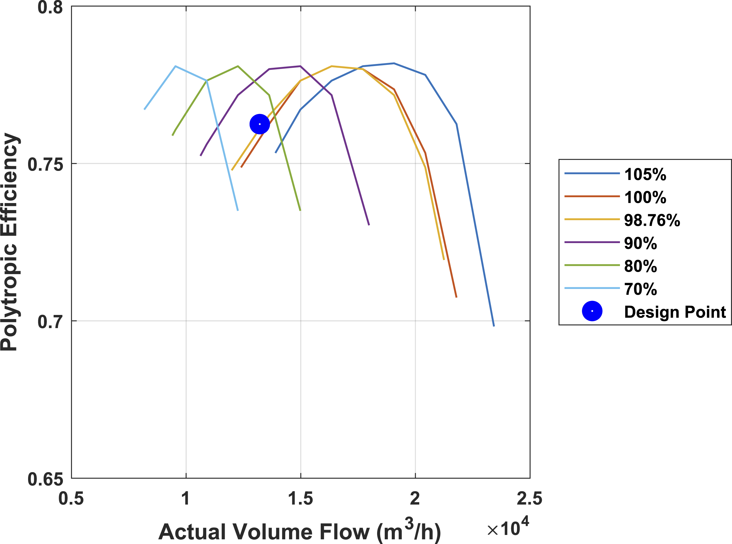
The gas compressor polytropic efficiency increases with the actual inlet volume flow rate until it reaches a maximum. Thereafter, it starts to decrease. Additionally, the working point at the design conditions of compressor station 3 has a polytropic efficiency approximately 2% lower than the maximum.
Figure 21 illustrates the variation in gas compressor power requirement at design and off-design conditions, as well as the actual inlet volume flow, at different rotational speeds on the gas compressor performance map for station location 3. Power curve for station 3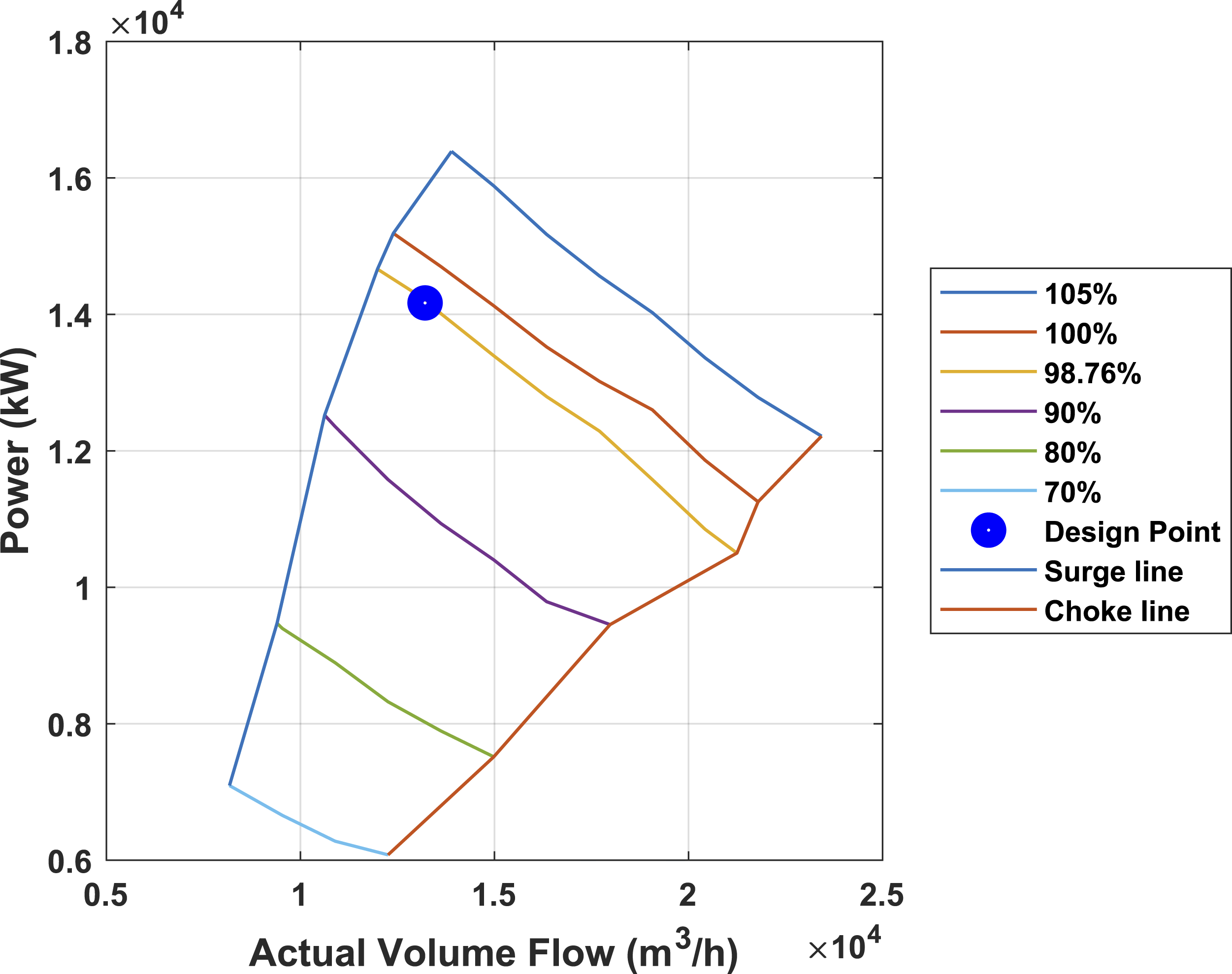
The results show an increase in gas compressor power and actual inlet volumetric flow rate as gas compressor shaft rotational speed increases. However, at a constant gas compressor shaft rotational speed, the gas volumetric flow rate decreases as the gas compressor power requirements increase. This arises from an increase in the polytropic head due to a rise in the gas flow temperature.
Impacts of operating points at varying flow conditions
Figures 22 and 23 illustrate the polytropic head and the power curves for station 2. They show operating points in different flow conditions. Polytropic head curve for station 2 showing operating points in different flow conditions. Power curve for station 2 showing operating points in different flow conditions.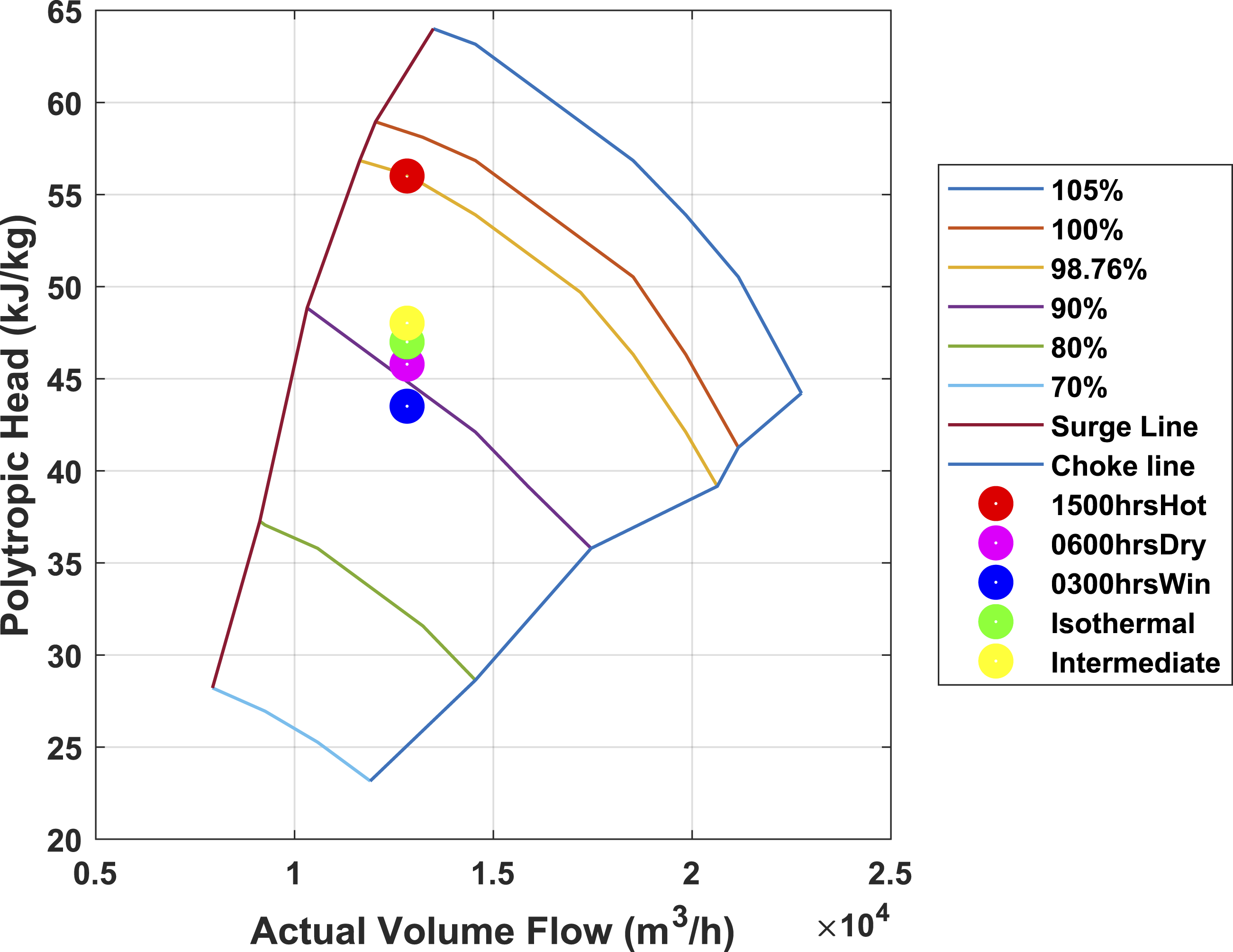
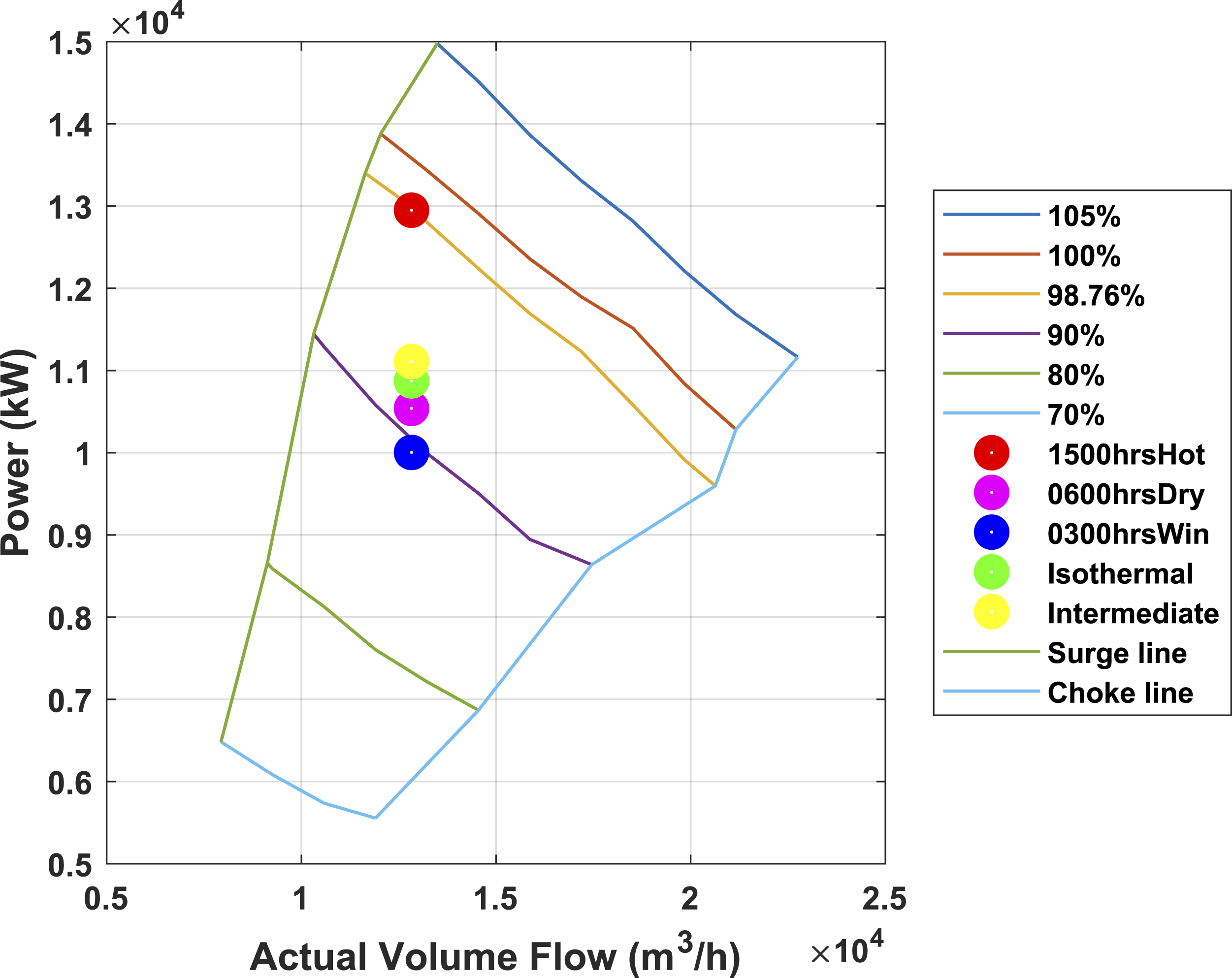
The results illustrate the effects of varying operating conditions at different points. A change in the location’s ambient temperature from 15:00 hours in the hot season to 06:00 hours in the dry season to 03:00 hours in the winter season for the non-isothermal flow conditions of scenario two leads to new operating points. These are illustrated in Figures 22 and 23. However, the gas compressor operating points are fixed at isothermal conditions (scenario 1) and at intermediate flow conditions (scenario 3). At these flow conditions, the temperatures are constant.
Peak, average, and minimum operating-point shifts for station 2
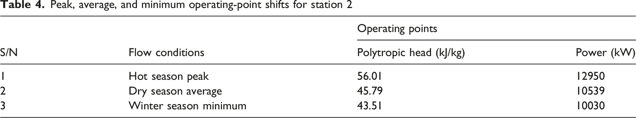
At 15:00 hours on a hot day, when the highest temperature is recorded, the polytropic head is 56.01 kJ/kg, and the required gas power is 12,950.0 kW. Similarly, at 06:00 hours of the day in the dry season, the polytropic head is 45.79 kJ/kg, and the required gas power is 10,539.0 kW. Furthermore, at 03:00 hours of the day during the winter season, when the temperature is at its lowest, the polytropic head is 43.51 kJ/kg, and the required gas power is 10,030.0 kW. The polytropic head shows a 28.7% operational range that is entirely invisible under the conventional isothermal assumption. Similarly, the peak non-isothermal power at Station 2 is approximately 19.1% above the isothermal estimate, while off-peak power is 7.75% below it. We observed that the gas power required increases with the polytropic head at a constant actual volume flow rate. This occurs due to a rise in the gas temperature. Furthermore, the gas compressor polytropic head increases by an average of 0.3% for each 1% increase in ambient temperature over the temperature range considered in this study. Therefore, the results show that, at constant gas composition and volume flow rate, the natural gas temperature significantly affects gas compressor performance.
Consequently, it is recommended that the working point be kept well away from the compressor stability curve. This study recommends a minimum surge margin of approximately 10% relative to the compressor surge line. This is important for steady operation and to prevent mechanical damage to the compressor. Therefore, the results have demonstrated that all operating points lie within the feasible regions for each scenario considered in this study. The subsequent section illustrates how the gas compressors are selected based on the results of the performance analysis using the TERA framework.
Gas compressor selection
Gas compressors are chosen based on the performance analysis and economic considerations. This analysis accounts for the highest ambient temperature, gas compression ratio, and power requirements for the gas compressors across all flow conditions considered in the scenarios. This includes decisions on the economic cost of the selected gas compressors. At each compressor station, four identical gas compressors are arranged in parallel. The baseline scenario includes 18 compressor stations along the natural gas pipeline route. Each gas compressor produces the same compression ratio and power and compresses an equivalent volume of natural gas. Figure 24 illustrates a schematic of gas compressors arranged in parallel. Parallel gas compressors arrangement schematic diagram.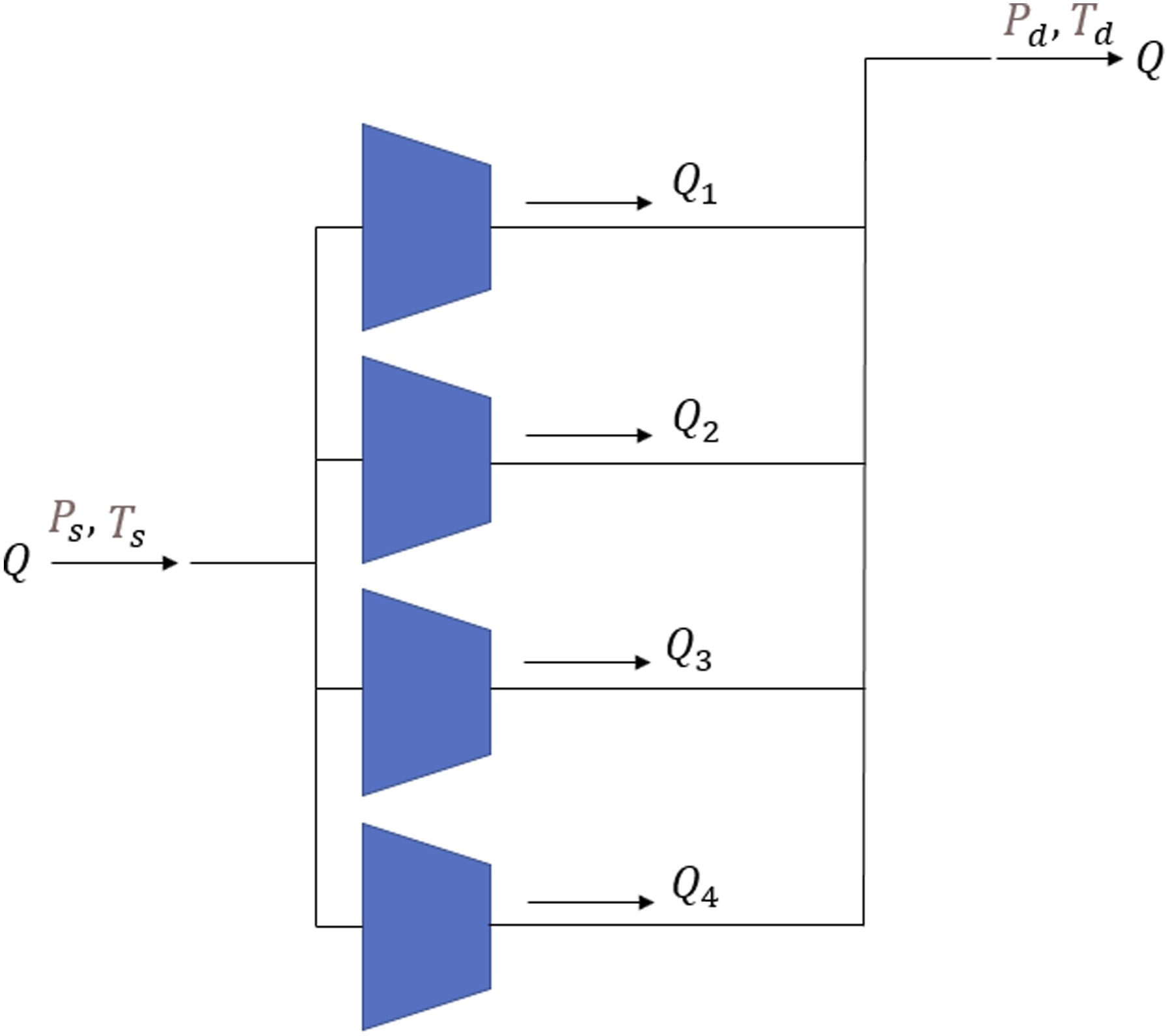
The significant volume flow rate required to be transported through the Trans-Saharan Gas Pipeline route necessitates the selection of parallel gas compressor arrangements. This selection has the advantage of lower gas compressor discharge temperatures than the series arrangement, as it eliminates the need for multiple compression ratios. Therefore, the total gas compressor discharge temperature for this selection will be equivalent to that of a single gas compressor installed at the compressor station with a similar compression ratio.
Figure 25 shows the gas compressor power requirement based on the maximum ambient temperature for all flow conditions described by scenarios 1, 2, and 3 at each compressor station location. Gas compressor power based on maximum ambient temperature in scenarios 1, 2, and 3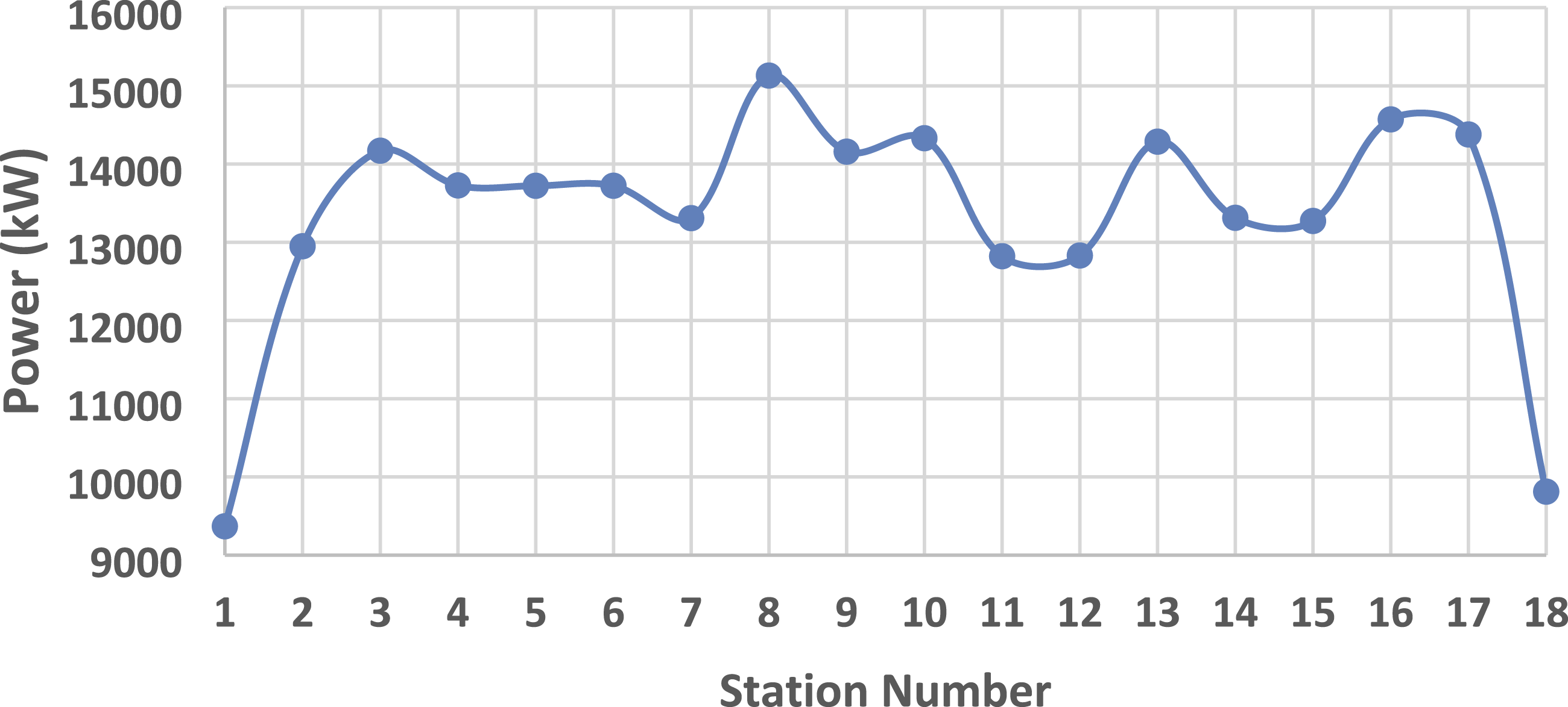
The first gas compressor station is assumed to operate under International Standard Atmosphere conditions. The maximum temperatures were observed at 15:00 hours of the day during the hot season of the year. These guidelines are used to select the appropriate gas compressor models in this study.
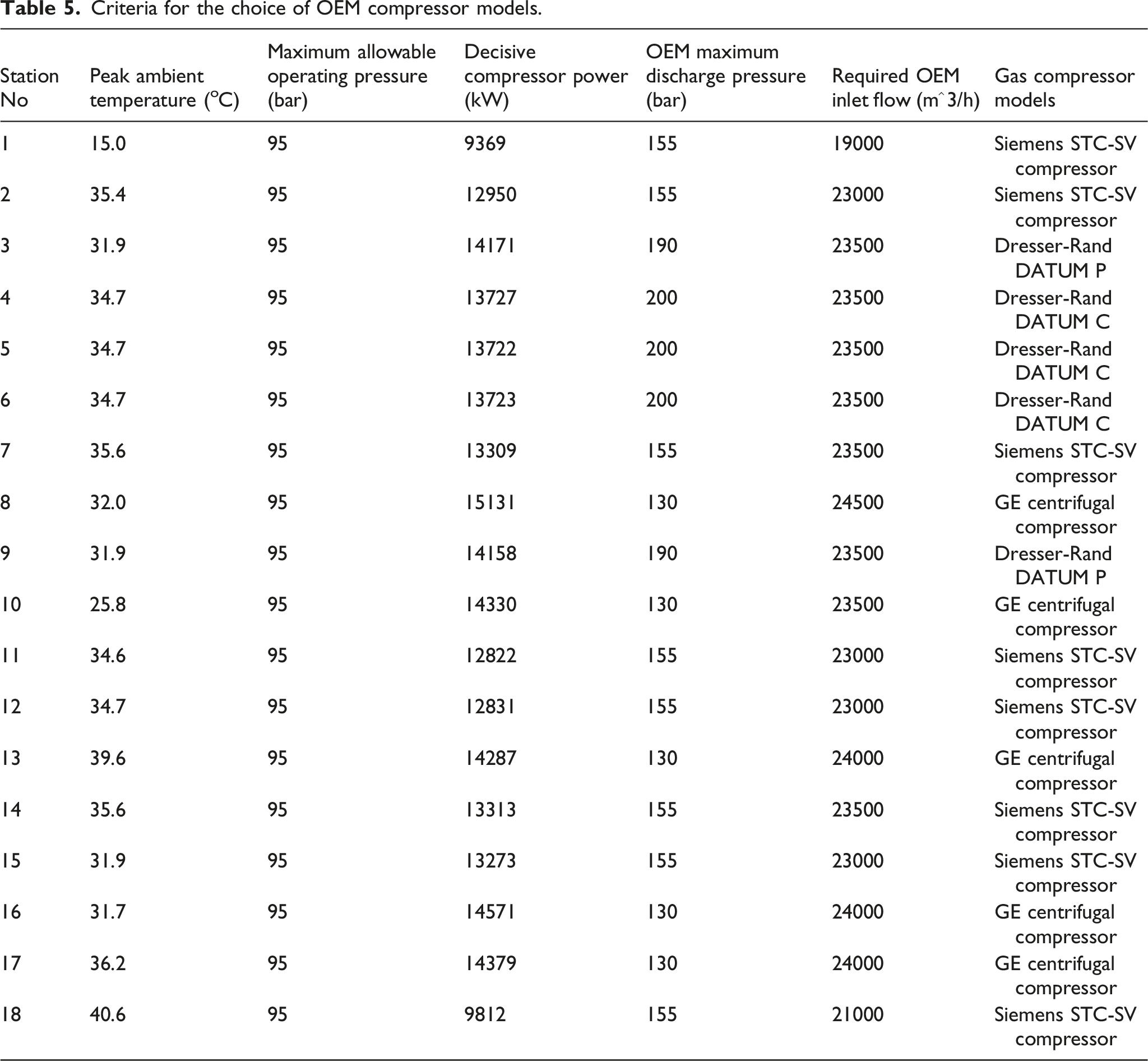
Four gas compressor models are chosen based on the gas compressor power requirements at all flow conditions described by scenarios 1, 2, and 3, while considering the economic implications of the selected models. These gas compressor models are inspired by: Siemens’ single-shaft pipeline compressor packages STC-SV compressor, General Electric centrifugal compressors, Dresser-Rand DATUM P, and DATUM C compressor trains. The gas compressor models are selected based on their small footprints, engine availability, and project lifecycle costs.
Criteria for the choice of OEM compressor models.
Gas turbine models are selected based on the gas compressor power requirements at all flow conditions. However, these are outside the scope of this study. Future studies will incorporate gas turbine performance analysis. The following section utilised a parametric sensitivity analysis to assess the effectiveness of the TERA framework outputs in response to variations in the gas compressor station’s key performance indicators.
Parametric sensitivity analysis
Parametric sensitivity of compressor power and polytropic head to ±5% variations in key input parameters at station 2 design point.
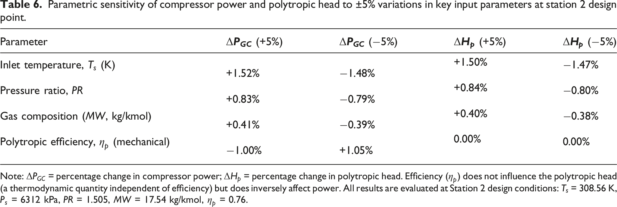
Note:
The results in Table 6 confirm that inlet temperature is the most influential parameter, with a ±5% perturbation producing a ±1.5% change in compressor power and an equivalent ±1.5% change in polytropic head. This finding is consistent with the diurnal power variation observed in the section analysing the gas compressor power at varying flow conditions at different station, where non-isothermal ambient fluctuations directly drive compressor demand. The pressure ratio ranks second in influence (±0.8%), followed by polytropic efficiency (±1.0% on power only) and gas composition through Variation of inlet temperature on compressor (a) pressure ratio (b) polytropic head (c) discharge temperature (d) efficiency (e) power.
Having performed a parametric sensitivity analysis to assess the robustness of the TERA framework, the following section translates the gas compressor power demand into operational costs to fully realise the techno-economic aspect of the TERA framework.
Techno-economic and operational impact analysis
The technical performance analysis presented in the preceding sections has direct and significant implications for the economic and operational viability of the compressor stations. To fully realise the “Techno-economic” aspect of the TERA framework, this section translates the gas compressor power requirements into operational costs, using the business electricity rate for Nigeria of USD 0.051 per kWh.89,90 However, this business electricity rate does not reflect location-specific pricing but is justified because it serves as a better approximation for financial modelling and scenarios comparison purposes. Particularly, since the project is in its conceptual phase.
The annual operational cost for each compressor station was calculated based on the power requirements from Scenario 1 (Isothermal) (see Table 3) using the formula: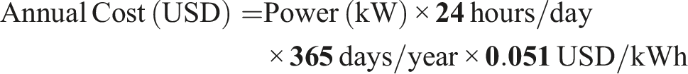
Annual operational costs for compressor stations based on Isothermal power requirements.
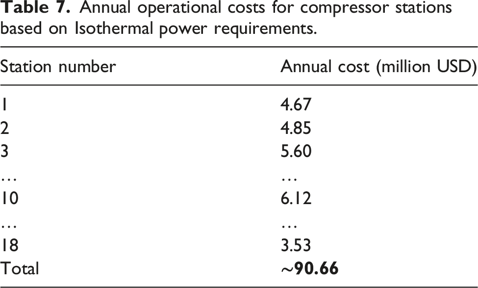
However, the critical finding from preceding sections is that power demand is not constant but fluctuates under real-world, non-isothermal conditions (Scenario 2). During the hottest part of the day (15:00 hours), power requirements can be significantly higher. A sensitivity analysis assuming a +10% power increase during daily peaks reveals that operational costs could be underestimated by over USD 56,000 per year for a single station, such as Station 3, totalling millions of dollars across the entire pipeline network. This demonstrates that the isothermal assumption, while simplifying design, risks substantial under-estimation of long-term operational expenditures (OPEX).
Furthermore, Nigeria’s electricity market is characterised by volatility, with prices influenced by factors such as exchange rates, gas prices, and regulatory changes.90,91 A sensitivity analysis of a ±10% change in the electricity rate would correspondingly alter the total annual cost by approximately ±USD 9.07 million, highlighting a significant financial risk that must be managed.
These economic insights lead to several strategic operational recommendations: • • •
Therefore, this economic analysis confirms that the non-isothermal model is not merely a technical exercise but a crucial tool for accurate financial forecasting, risk assessment, and optimising the total lifecycle cost of the pipeline system.
Conclusion
This study successfully implemented a Techno-Economic and Environmental Risk Analysis (TERA) framework to evaluate the performance of gas compressor stations under three distinct thermal-flow scenarios for natural gas pipelines. The comprehensive analysis reveals that: • The assumption of gas temperature behaviour (i.e., isothermal, intermediate, or non-isothermal) fundamentally affects pipeline pressure drops, compressor suction conditions, and power requirements. Non-isothermal analysis most accurately captures real-world operational dynamics, in which an increase in gas flow temperature leads to an increase in pressure drop, and vice versa. • Compressor stations with long pipeline segments and high elevation gain (e.g., Station 10) experience the most challenging operating conditions, characterised by the lowest suction pressures, highest compression ratios, and thus, the highest power requirements. • Under realistic non-isothermal conditions, compressor power exhibits substantial diurnal and seasonal fluctuations, peaking at 15:00 hours during hot seasons and reaching minimums at 06:00 hours during cold seasons. This variability necessitates equipment sizing based on peak demand rather than average conditions. • The estimated annual operational cost of $90 million under isothermal conditions is subject to significant increases due to non-isothermal fluctuations and regional electricity price volatility, highlighting critical financial planning considerations.
The analytical methodology developed in MATLAB demonstrated excellent agreement with industry-standard Aspen HYSYS simulations, validating its accuracy for compressor performance analysis. The maximum absolute percentage difference in power calculations was merely 0.348% at Station 18 - well within acceptable engineering tolerances. This strong correlation confirms the reliability of the developed models for natural gas pipeline applications. Furthermore, the investigated scenarios comprehensively represent realistic operating conditions encountered in long-distance transmission pipelines, encompassing the full spectrum of temperature variations across geographical routes. Consequently, this study provides pipeline designers with a validated framework for optimising compressor station design and operation in both new projects and existing infrastructure.
Limitations and future research directions
This study has evaluated the performance of the gas compressor and pipeline system under various gas flow temperature conditions. However, the analysis was performed under the assumption that the gas-flow temperature is equivalent to the location’s ambient temperature at the compressor station’s suction or discharge point. Future studies could examine the derivation of equations describing the transient flow of gas in pipes. In this approach, the gas temperature will be a function of the pipe length. This would be computed using a numerical model developed to incorporate the energy equation. The analysis would yield a time-dependent temperature profile based on transient, non-isothermal gas flow in the natural gas pipeline. The uncertainty analysis identifies the compressibility factor as the dominant contributor to model uncertainty. Future work will incorporate improvements to the compressibility factor through better gas-composition measurements and higher-fidelity real-gas models, such as GERG-2008.
Footnotes
Acknowledgements
The authors are grateful to the Petroleum Technology Development Fund of Nigeria (PTDF/ED/PHD/OOB/1386/18), for funding the PhD research that has led to the publication of this paper.
Declaration of conflicting interests
The authors declared no potential conflicts of interest with respect to the research, authorship, and/or publication of this article.
Funding
The authors disclosed receipt of the following financial support for the research, authorship, and/or publication of this article: Petroleum Technology Development Fund (PTDF/ED/PHD/OOB/1386/18).