
Abstract
Bifacial photovoltaic cells can produce electricity from incoming solar radiation on both sides. These cells have a strong potential to reduce electricity generation costs and may play an important role in the energy system of the future. However, today, these cells are mostly deployed with one side receiving only ground reflection, which leads to a profound sub-optimal utilization of one of the sides of the bifacial cells. Concentration allows a better usage of the potential of bifacial cells, which can lead to a lower cost per kWh. However, concentration also adds complexity due to the higher temperatures reached which add the requirement of cooling in order to achieve higher outputs. This way, this paper focuses on the effectiveness of forced air circulation methods by comparing the thermal performance of three specific concentrating bi-facial collector designs. This paper developed a computational model, using ANSYS Fluent intending to assess the thermal performance of a covered concentrating collector with bifacial Photovoltaic (PV) cells. These results have then been validated by outdoor measurements. Results show that even a simple natural ventilation mechanism such as removing the side gable can effectively reduce the receiver temperature, thus resulting in favourable cell operation conditions when compared to the case of an airtight collector. Therefore, compared with a standard model, a decrease of 13.5% on the cell operating temperature was reported when the side gables are removed. However, when forced ventilation is apllied a 22.8% reduction on temperature is found compared to the standard air-tight model. The validated CFD model has proven to be a useful and robust tool for the thermal analysis of solar concentrating systems.
Keywords
Introduction
The addition of concentrators to Photovoltaic (PV) cells can allow achieving higher cell efficiency, and consequentially has the potential to decrease the electrical generation costs. This reduction benefit is far more pronounced when the photovoltaic cells utilized in the PV concentrator are bifacial. Bifacial PV cells can produce electricity on both sides if they are exposed to sunlight. Bifacial PV cells have a strong potential to reduce electricity generation costs and may play an important role in the energy system of the future. However, today, these cells are mostly placed in transparent PV panels that are installed with one side only receiving ground reflection. This leads to a profound sub-optimal utilization of one of the sides of the bifacial cells, since one side receives a maximum solar radiation of around 150 W/m2 depending on ground reflectance, while the other side receives a maximum of around 1100 W/m2, under optimal incidence conditions. This way, concentration allows for a better usage of the potential of bifacial cells by allowing both sides of the cells to receive a significantly improved solar radiation profile, which in turns is expected to lead to higher annual outputs and lower kWh generation costs. However, one significant drawback is that concentration also adds complexity to the panel since this leads to higher panel temperatures and requires cooling in order to achieve higher outputs. In concentrating panels, cooling is essential since today the PV cells typically show a performance reduction of around 0.35%/1°C. 1 This way, this paper focuses on the effectiveness of forced air circulation methods by comparing the thermal performance of three specific concentrating bi-facial collector designs.
According to, 2 concentrators can reduce land utilization as well as area-related costs. It is also known that output power and efficiency decrease with the operating temperature. To attenuate the reduction in its efficiency several means for temperature control of the PV cell collector have been studied.3–6 An in-depth review of cooling techniques has been conducted by, 7 which highlights the benefits of different cooling strategies in standard PV panels. However, the authors did not find the same studies for air forced cooling on concentrating bifacial PV panels. 8
Studied the influence of the incidence angle on the temperature of the cover and back glass, as well as on the PV cell silicone temperature. They performed experiments and CFD calculations for different angles of incidences such as 0°, 10°, 20°, 30° and 40°. Crossed Parabolic was the type of concentrator analyzed. 9
Carried out tests on three prototypes of compound parabolic concentrators (CPC) collectors of non-cooled bifacial PV cells. Results showed a cell temperature of 88°C on a glass-covered outdoor installed collector on a sunny day with 28°C of ambient temperature. The dependence of electrical efficiency on temperature was reported to be −0.51%/K. The authors pointed out several drawbacks of concentrating photovoltaics, one of them is the PV cell efficiency being reduced by non-uniform light and the other is the efficiency reduction as a consequence of increasing temperature from concentration. Because of this, reflector shapes and the normal operating cell temperature of the collector must be carefully considered during the design of these types of solar collectors. 10
Investigated experimentally and numerically the influence of longitudinal and transversal solar incidence angle on the output of a Concentrating Photovoltaic (CPV) solar collector. Simulations were compared with the experiments. Results showed a direct relationship between the collector concentration ratio and the operating temperature of the cells. The authors pointed out the importance of cell cooling, and they suggested that the ventilation of the cells was a path to enhance the collector performance. 11
Used a CFD model to investigate the effect the tilt and the wind velocity have on the electric output of a PV collector. The CFD code was used also to predict the temperature distribution on the collector. Results showed that simulations can be used as a preliminary tool for estimating the PV efficiency under different mounting orientations. 12
Reviewed various methods found in literature to enhance the electric output of a concentrating PV cell by lowering its operating temperature. They also tested an innovative design to cool cells based on pulsating technology. Findings of a set of experiments show that applying pulsating is more efficient than the conventional continuous flow. However, concerns arose regarding the pulsation vibration experienced during the experiments that should be taken with caution when employing this technology.
There is much literature on the topic of cooling techniques for PV panels, however to the best of the author´s knowledge there is no publication covering the combined technologies of forced air cooling of bifacial on concentrating PV panels.
This paper conducts thermal analysis on three different model configurations on a parabolic concentrator coupled with bifacial PV cells. Outdoor experimental tests were carried out on a production model, which served as a means for the validation of a numerical code. The tested model was considered the reference case as it mimics the standard, airtight collector with no assisted cooling. Validated simulations were then extended to study other different collector configurations. The main geometry of the collector (i.e. concentration ratio, the position of the bifacial PV cells, and reflector design) as well as test ambient conditions (i.e. irradiance and the ambient temperature) were constant during the simulations. Two strategies for cell cooling are proposed and the performance of each one was analyzed and compared to the standard case.
Methods and experiments
To validate the numerical results, a set of reliable and high-quality experimental data was necessary.
Experimental set-Up
Several tests have been performed on a CPC collector with dimensions of 528 mm × 2250 mm × 250 mm (x,y,z), as shown in Figure 1. The collector is covered by a 4 mm low-iron solar glass, with a weighted solar light transmittance of 95% at wavelengths of 600 nm. The parabolic trough is made of 2 mm aluminum with a weighted solar light reflectivity of 93%. The receiver comprises a set of five layers: two 0.5 mm cells laminated on each side of a 5 mm plexiglass plate. Two exterior cell silicone coatings of 0.5 mm were also used on top of each cell string for protective purposes. An overall view of the solar collector and the instrumentation used is presented in Figure 1. Solar collector overall view. The points above the shaded plan show the position of the thermocouples and the anemometer used in this study. Dimensions are in mm.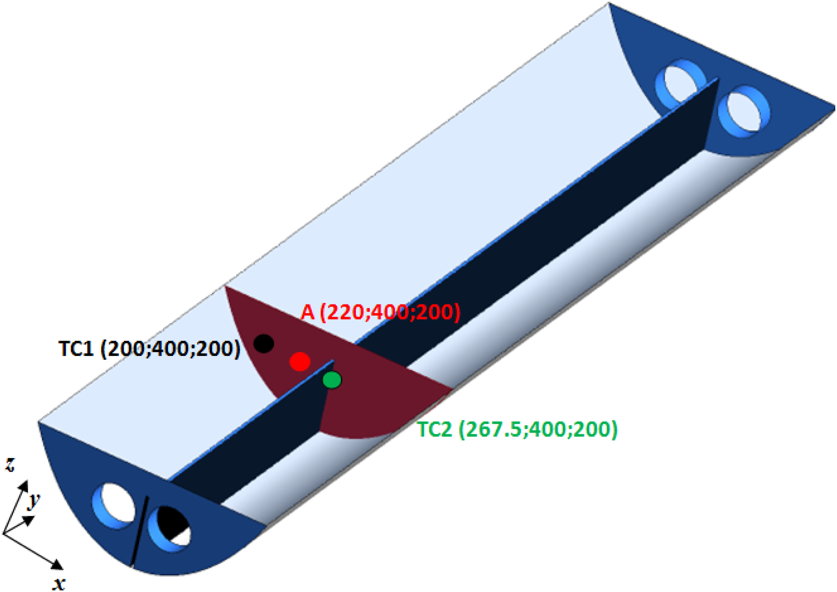
Two K-type thermocouples coded as TC1 and TC2 have been placed accordingly to Figure 1 in order to measure the air and cell temperature, respectively. A data-logger from Pico Technology (model TC-08) has been used to register the different cell temperatures along with the test duration. Additionally, a hot wire anemometer (Swema Air, model 300) and two pyranometers Kipp and Zonen (model CMP3 for diffuse radiation and CMP6 for global radiation measurements) have been used. The following Figure 2 shows the experimental setup installed in the test rig. View of the experimental set-up.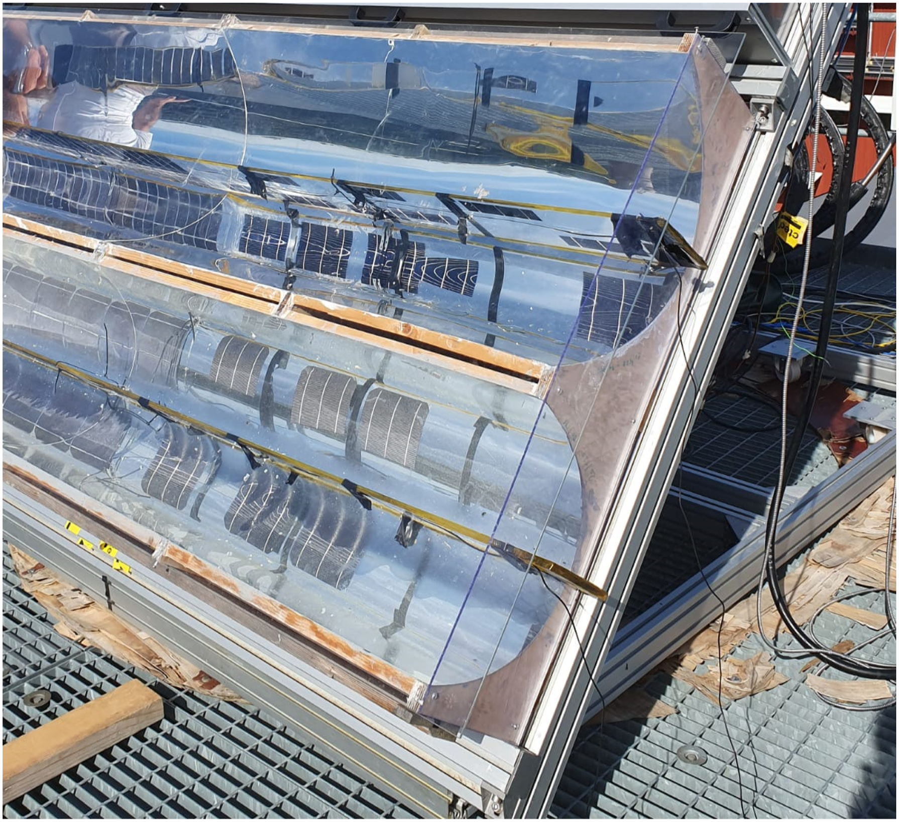
The uncertainties of measurement were estimated using a B-type methodology, 13 i.e. relying on the data provided by each instrument´s manufacturer. Expanded uncertainties using a 95% confidence interval were found: UT95 = ±0.11 K for the temperature sensors, Uv95 = ±0.03 m/s for the air velocity sensors and US95 = ±25 W/m2 for the solar irradiance sensors.
Experimental procedure
The CPV solar collector was installed on a solar collector stand at the University of Gävle laboratory in Sweden and the outdoor testing procedure has been performed during August 2019. The optimum collector tilt angle was found to be around 55° for the specific collector-testing period as the solar altitude varies throughout the whole month of August. As Gävle University is located in the northern hemisphere, the collector has been south-oriented.
As instantaneous readings were recorded, it is necessary to stabilize the measurements, therefore it has been given some short period to fulfill this requirement. The outdoor measurements were recorded from 11 a.m. and 1 p.m. as the projected solar altitude is fairly constant throughout this time. Both global and diffuse solar radiation was measured by two pyranometers located in the same collector plane and stored in a data logger from Campbell Scientific CR1000.
The CFD model
Analytical solution methods are limited to highly simplified problems in simple geometries.
14
Therefore, CFD software packages available are a powerfull tool for more realistic models when analysing fluid mechanics and heat transfer. The physical phenomena involved in a CPV collector is characterized by complex mechanisms like radiation, turbulence or unsteadiness thus the preference for using CFD methods in this investigation. For this numerical study, a commercial CFD code, Ansys-Fluent (release 17.0) has been used, namely to predict the temperature distribution and flow pattern in a CPC collector. Figure 3 shows an overall picture of the complete CPV solar collector model used in the simulations. Model of the glass-covered concentrating collector studied.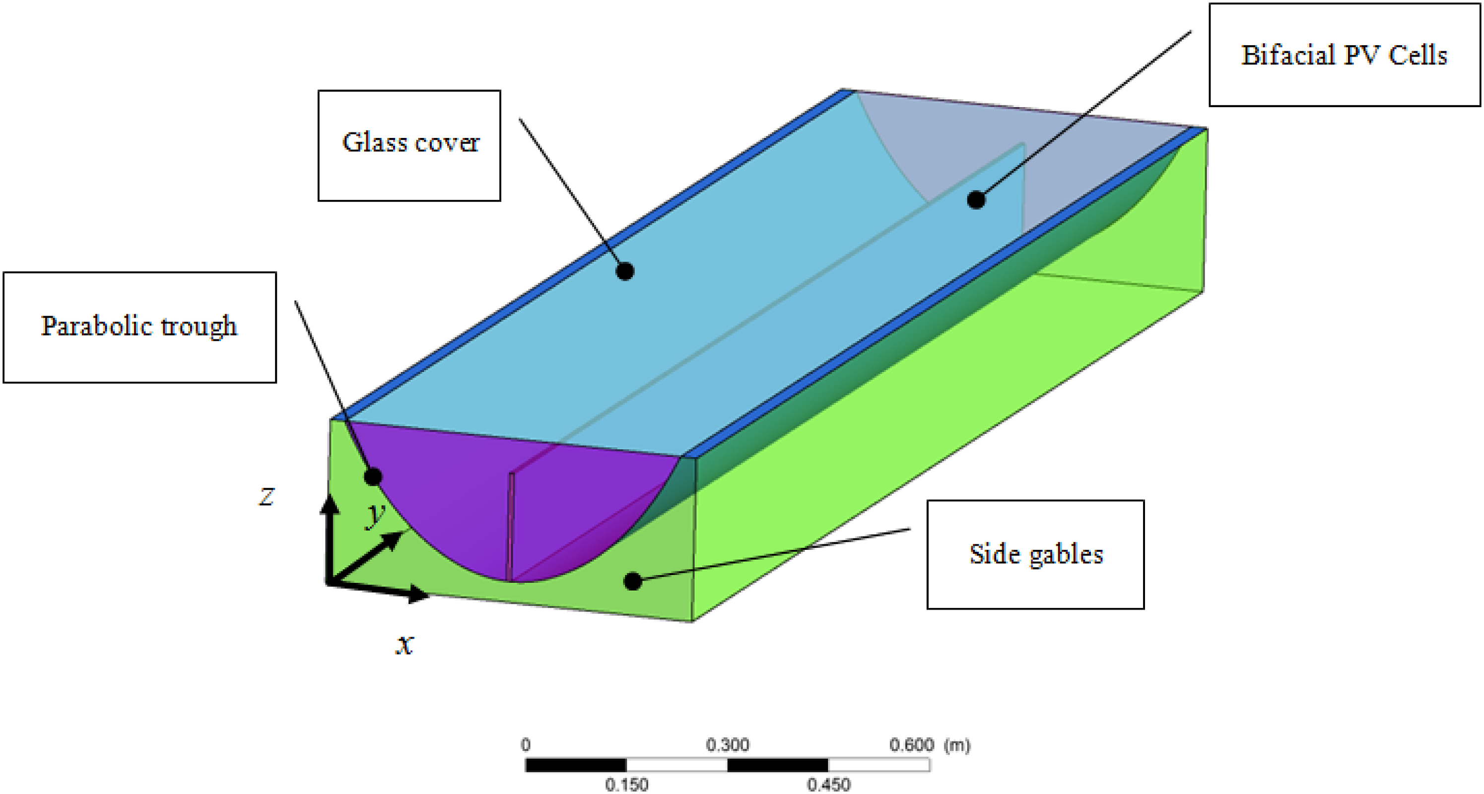
Outdoor tests have been carried out to validate the simulation results. After the code validation has been carried out, other layout configurations have been proposed and studied numerically to investigate their ability to decrease the PV cell operating temperature and thus increasing the overall PV production. Case 1 corresponds to the collector tested. In case 2 the lateral gables have been removed, and in case 3 a pair of fans were installed in one of the gables of the collector. The results are discussed in The Results and discussion. Figure 4 illustrates the three cases studied. A cross-section view (plane zx) of the three cases studied and each one’s composition (not to scale).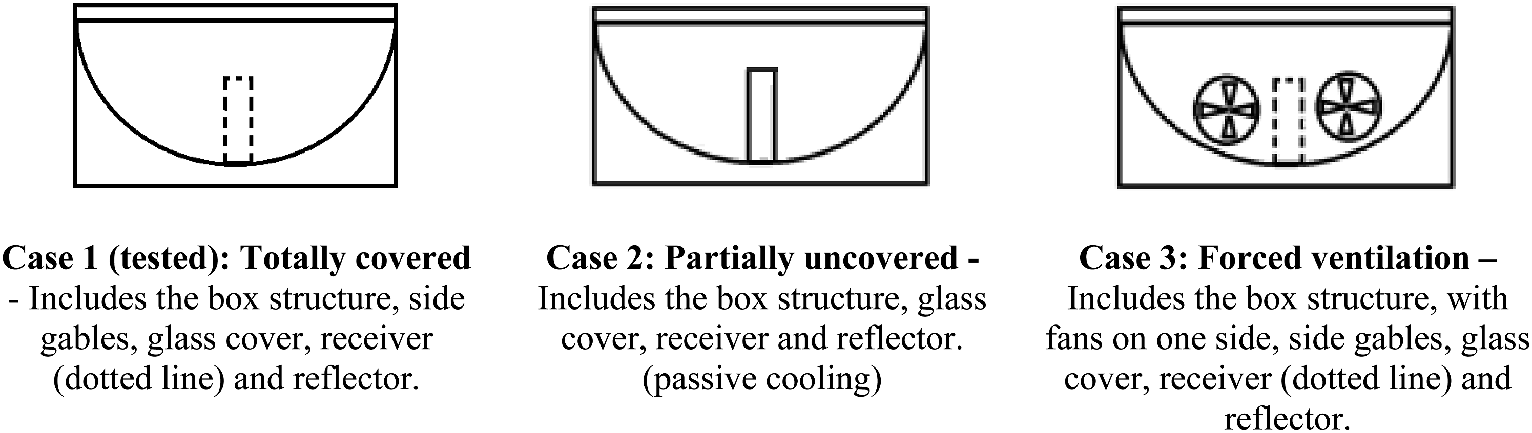
The data has been obtained from solving the mass, momentum and energy equations. Furthermore, additional quantities from turbulence models were used, as a result of the Reynolds Average Navier Stokes approach. Equations were extended to the third dimension in space.
CFD Set-Up
Turbulence
Showed that the accuracy in the prediction of turbulent flow behavior is a consequence of the accuracy of the turbulence models used in this same forecast. 15 Thus turbulence is a complex problem that has to be tackled. It affects mainly the numerical analysis, although it might also introduce uncertainties in the experimental analysis as well. The standard k-ε was the model selected in this study due to the good performance achieved in similar applications. This model has been widely used in studies of fluid mechanics and heat transfer, 16 because it combines relative robustness of results and accuracy, without being computably expensive. It is a semi-empirical model of two equations in which the turbulent transport variables are the turbulent kinetic energy (k) and the dissipation rate (ε). The default turbulence model constants available in the CFD code were left unchanged.
The law-of-the-wall is normally used to avoid a very fine mesh in the vicinity of the solid boundaries, although more accurate predictions can be obtained with the refinement of the mesh in this zone, together with an appropriate turbulence model selection such as a low Reynolds number turbulence model. In order to achieve a higher degree of accuracy in the simulations performed, an enhanced wall treatment has been employed in this study. It comprises a two-layer model 17 in which the transition between the zones is made by applying a blending function. 18
Buoyancy
In the presence of heat transfer to the air, a variation of its density will occur as a consequence of its heating. The gravitational force will act under different intensities, promoting the motion of the particles. Natural convection is possible to be modeled numerically by the Ansys-Fluent software. In those circumstances, the Boussinesq approach is normally adopted. This approximation treats density as constant in all but the momentum equation. In it, the density property will be expressed as a function of temperature

Where ρ0 designates the reference air density and T 0 is the temperature understudy, β the air expansion coefficient and g the gravitational acceleration. This approach originates results with acceptable deviations as long as the variations in the air temperature are comprised of β (T-T 0 ) <<1 interval, which is the case in this study. For the buoyancy modeling to be implemented, the gravitational acceleration has also to be introduced, which, because of the tilt, will act both in the x-axis and z-axis with the same magnitude as the gravitational acceleration of −9.81 m/s2.
Boundary conditions
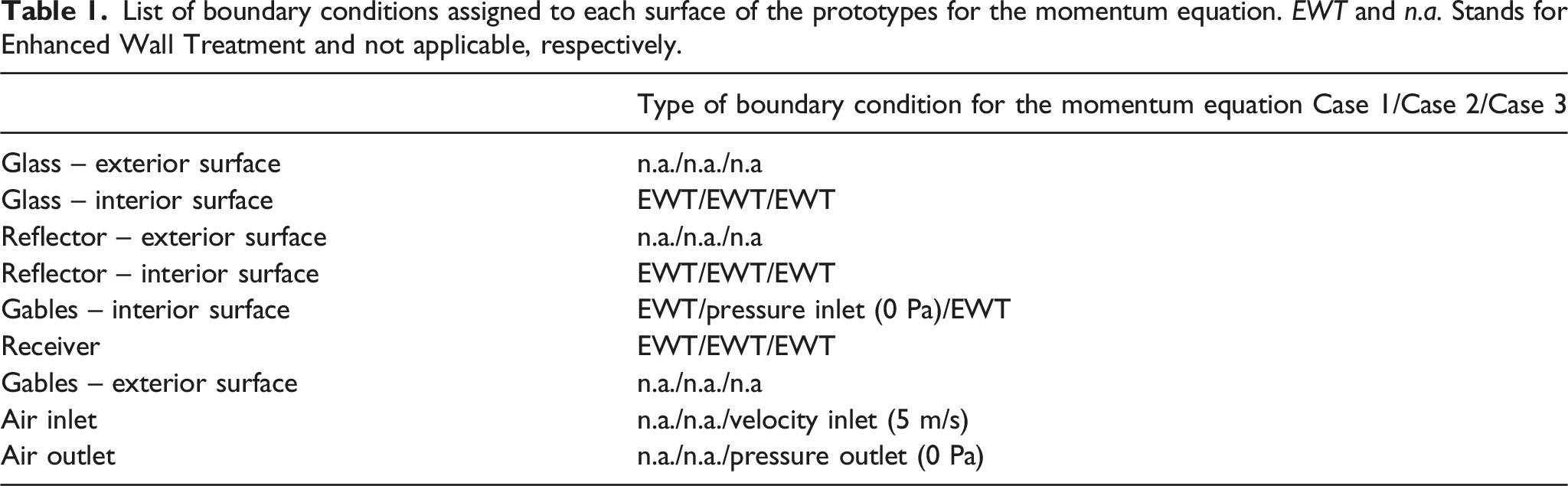
List of boundary conditions assigned to each surface of the prototypes for the momentum equation. EWT and n.a. Stands for Enhanced Wall Treatment and not applicable, respectively.
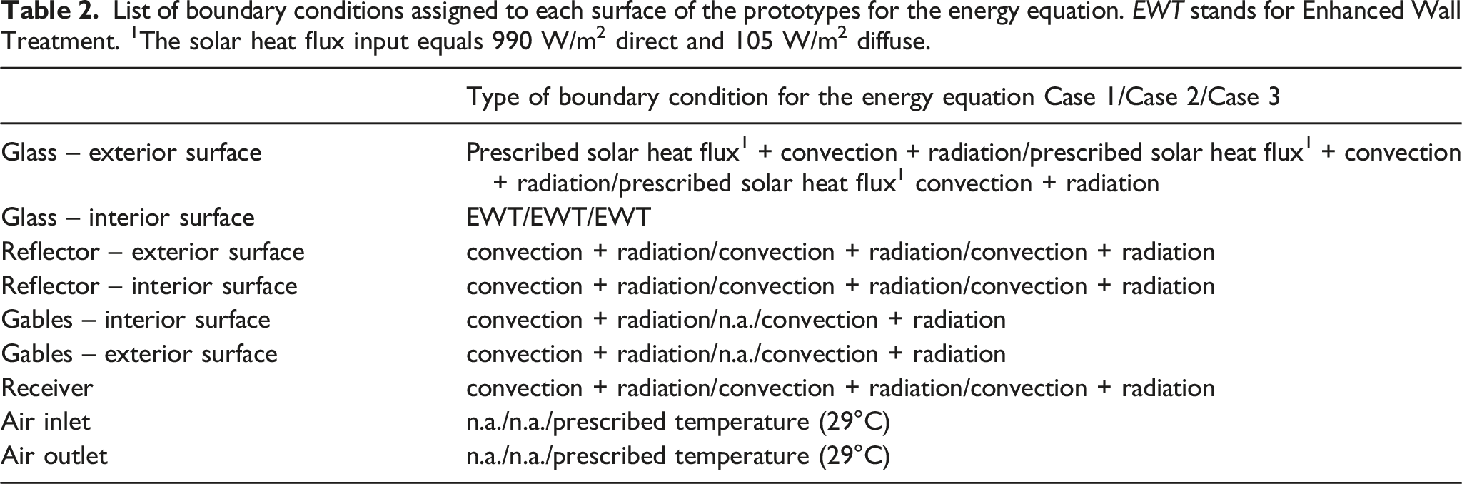
List of boundary conditions assigned to each surface of the prototypes for the energy equation. EWT stands for Enhanced Wall Treatment. 1The solar heat flux input equals 990 W/m2 direct and 105 W/m2 diffuse.
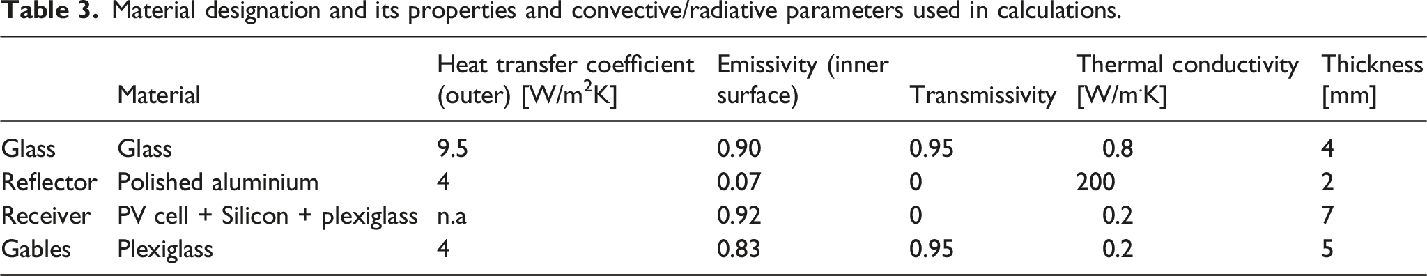
Material designation and its properties and convective/radiative parameters used in calculations.
The heat conduction is calculated by Ansys-Fluent software on solid domains. For this purpose, a mesh was created in those regions. In order to improve the speed of calculation, a mesh was generated in the receiver core only and, in the case of the glass, gables, and reflector this approach was not used. Instead, a thickness was defined for these surfaces along with the specification of the material.
Radiation
In the presence of heat transfer by natural convection, the radiation component may represent a significant fraction of the heat transferred. 14 Therefore, the radiation emitted by the bodies will be absorbed by the surrounding surfaces conditioning the final balance of energy.
The Solar Model
The CFD code enables the calculation of a heat source coming from the sun to predict the effects on the domain. This is accomplished by defining a beam that is modeled using the sun position vector and illumination parameters. The resulting heat flux is coupled to the calculation via a source term in the energy equation.
The simulations were carried out using the Discrete Ordinates radiation model. Inputs of 990 W/m2 of direct radiation, as well as 105 W/m2 of diffuse radiation, were considered as these were the magnitude of each variable, registered by the pyranometers at the time experiments were made. This way simulations are hereby reproducing the test reference conditions (i.e. at noon). The sun direction vector was taken as pointing over the z-axis only. Therefore, the model assumes the incident solar radiation is striking the collector perpendicularly (i.e. at normal incidence).
Grid generation
The geometric model used in the CFD simulations was a simplified representation of the reduced-scale test facility. The computational domain includes the space occupied by the air, and the interior of the receiver, which is assumed to be homogeneous. Only the energy equation is solved in the interior of the receiver, as in this region heat conduction takes place solely, the velocity being equal to zero.
As shown in Figure 5, tetrahedral elements were used in the fluid domain while hexahedral elements were preferred for the solid domains of the receiver. When modeling the boundary layer, inflation was created in the fluid domain, namely in the interfaces with solid domains, using transition ratios of 1.1 and 1.2. Mesh used in the calculations taken in a plane at y = 1000 mm.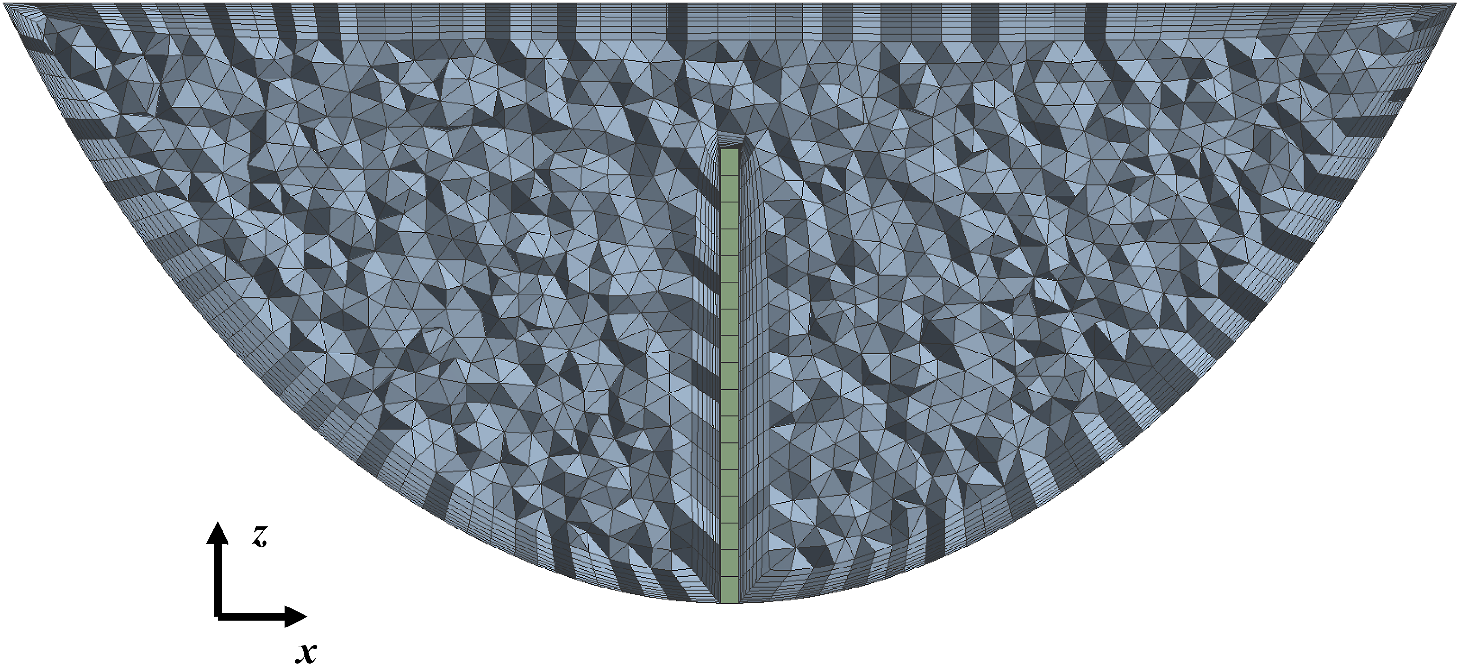
Grid independence study
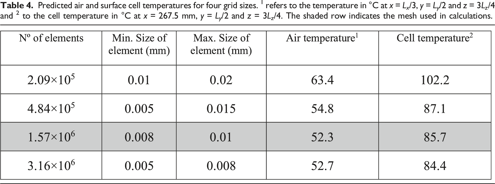
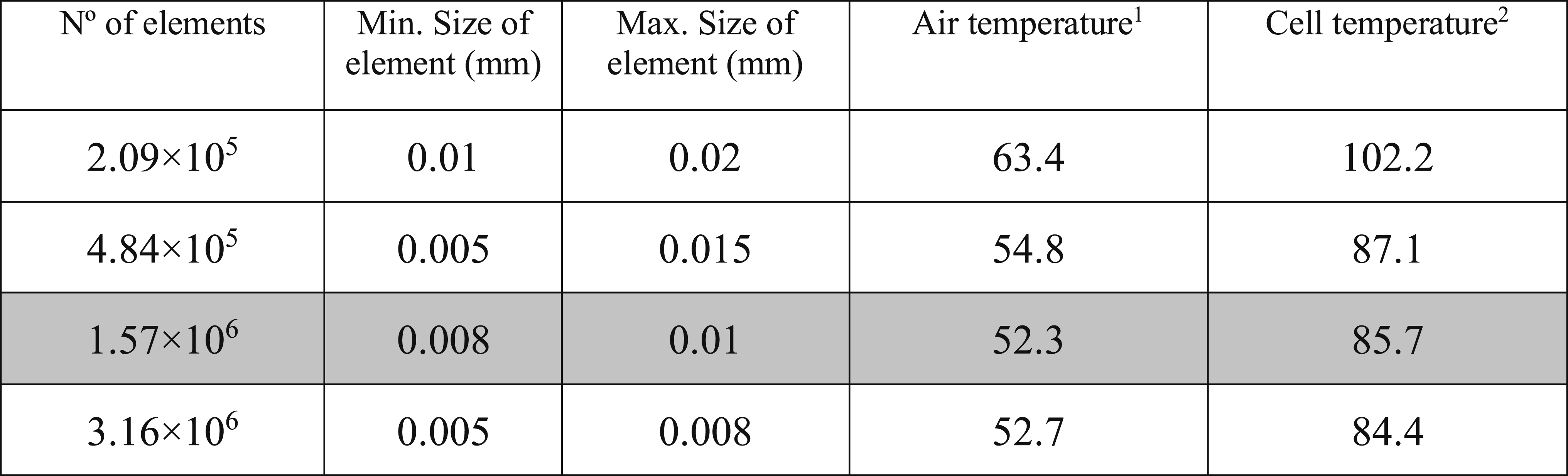
Predicted air and surface cell temperatures for four grid sizes. 1 refers to the temperature in °C at x = L x /3, y = L y /2 and z = 3L z /4 and 2 to the cell temperature in °C at x = 267.5 mm, y = L y /2 and z = 3L z /4. The shaded row indicates the mesh used in calculations.
Numerical solution algorithm
The finite volume method was used to solve the governing equations. The discretization of the convective terms of the momentum, energy and turbulence equations was done using the second-order upwind numerical scheme. The solver was set to steady-state and pressure-based type. The pressure-velocity coupling was determined by the SIMPLE algorithm. A convergence criterion relied on the magnitude of the unscaled residuals. Therefore values of 10−3 were used for the residuals of continuity, momentum and turbulence and 10−6 for the energy and radiation equations. Besides this standard practice, there was also an additional analysis of monitoring the temperature integral over a plane, over the iteration process, as a complementary criterion when judging convergence. Using both strategies implies that the solution is only considered to be converged when the magnitude of the residuals had been achieved and the evolution of the temperature integral monitor had reached a plateau.
Solver settings
The 3-D model was incorporated on Ansys-Fluent software (release 17.0), where the momentum, energy, radiation and turbulence equations were calculated. The solver general settings were defined as an incompressible steady regime. The discretization of the momentum, energy and turbulence equations was processed using second-order upwind type numerical schemes.
Results and discussion
Case 1
Air and cell temperature
As a preliminary consideration, it should be noted that the collector was tilted 55° during the simulation according to the experimental set-up, and for a better interpretation of the results, the figures on this and in the following sections display the collector on a non rotated position.
The predicted temperature contours, as well as the measurements, are shown in Figure 6 for case 1 in a plane at y = 400 mm. The air temperature ranged between 33.2°C and 64.5°C, whereas the cell temperature reaches 74.8°C in the base. The lower temperature found in this region of the collector is due to the heat sink effect caused by the connection between the cells and the parabolic trough. On the other hand, the cell temperature increases up to 88.1°C at the top. In the tests, temperatures of 53.4°C and 93.7°C were found in thermocouples TC1 and TC2, respectively, showing a good correlation between measured and simulated results. Thermal stratification is also reported in the calculated results, as this phenomenon is expected to occur on a tilted collector - air temperature differences of 35°C between the upper and lower regions of the cavity are observed in the simulations. Predicted and measured temperature contours in a plane at y = 400 mm for the case 1.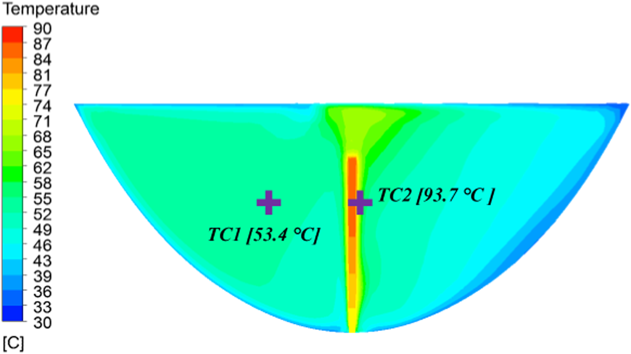
Figure 7 presents the calculated temperature profiles in the y and z directions for case 1. Horizontal profiles are coded here as HA for the air temperature and HC for the cell surface temperature followed by a sequential number. VA and VC show the equivalent results but for vertical profiles. It can be seen that the temperatures over the HA1 profile are always higher than over HA2. This is a result of the tilt of the collector, which leads to a specific stratification of air temperatures in its upper zone, a fact already discussed when the analysis of Figure 6. Regarding the distribution over z axis, it is noticeable, by the analysis of the vertical profiles of Figure 7 that the maximum temperatures of the cell and the air are achieved for the highest heights i.e. for z = 0.20 m and z = 0.23 m, respectively. Calculated temperature profiles in the air and cells over y and z directions for case 1.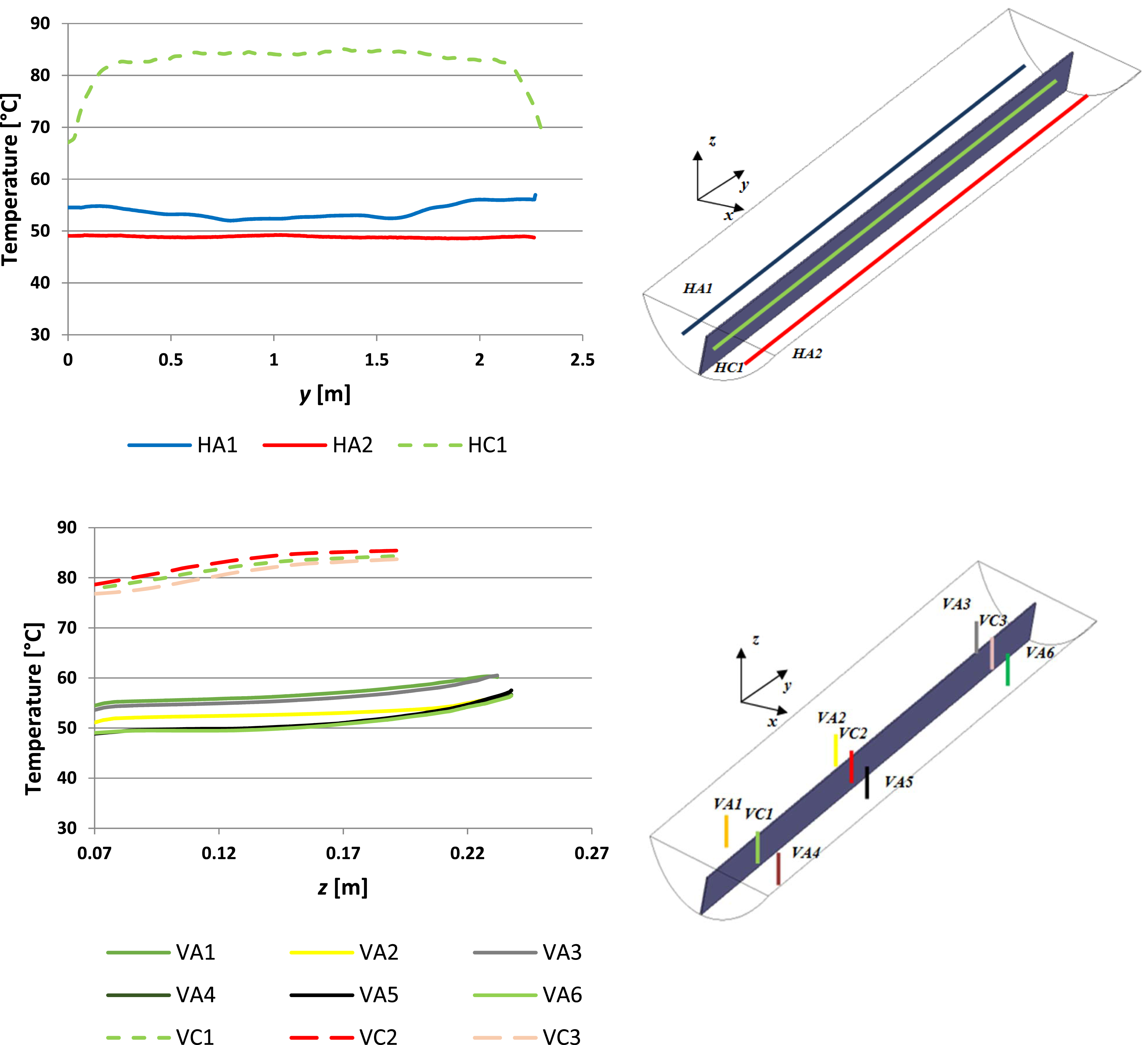
This case presents the highest temperatures in both the receiver and the surrounding zone, as expected, due to the greenhouse effect created by the presence of the glass. This way, this collector design presents the less favorable operating conditions for the PV cells.
Air velocity
Figure 8 shows the predicted velocity vectors and magnitude contours as well as the measured data by the anemometer A. Predicted and measured velocity contours in a plane at y = 400 mm for the case 1. The cross indicates the measurement result while the remaining is simulated.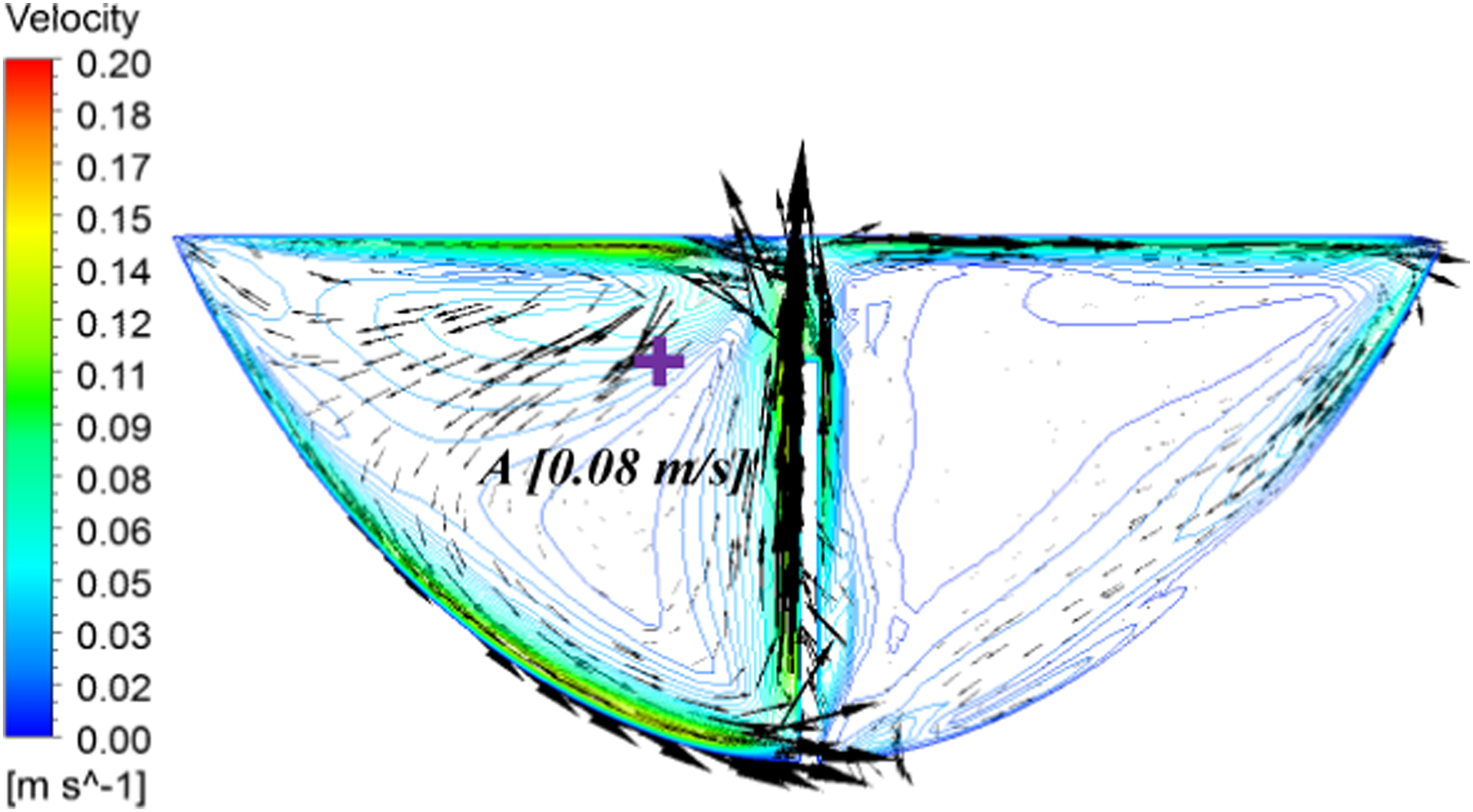
Comparing the upper and lower zones of the collector delimited by the receiver, asymmetric distribution of the magnitude of this variable can be spotted in the simulations. That is to say that in the upper zone much higher velocities are found than on the other half of the collector. Furthermore, the formation of a vortex on the upper side of the collector is noticeable. This is due to the higher temperature differences between the air (which is hotter in this part of the cavity than in the rest of the collector) and the other collector surfaces - glass and reflector. The highest velocity gradients are happening in the gap between the receiver and the glass - magnitudes between 0.12 and 0.17 m/s are encountered in this region.
Figure 9 presents the calculated air velocity profiles for case 1 over y and z directions. Identification of profiles adopts the same codification that was used for the temperature profiles i.e. horizontal profiles as HA and as VA for vertical profiles, followed by a sequential number. In this analysis the profiles relative to the cells are not considered since the velocity at its surface is equal to zero due to the no-slip condition. Calculated velocity profiles in the air over two and six lines over y and z directions, respectively, for the case 1.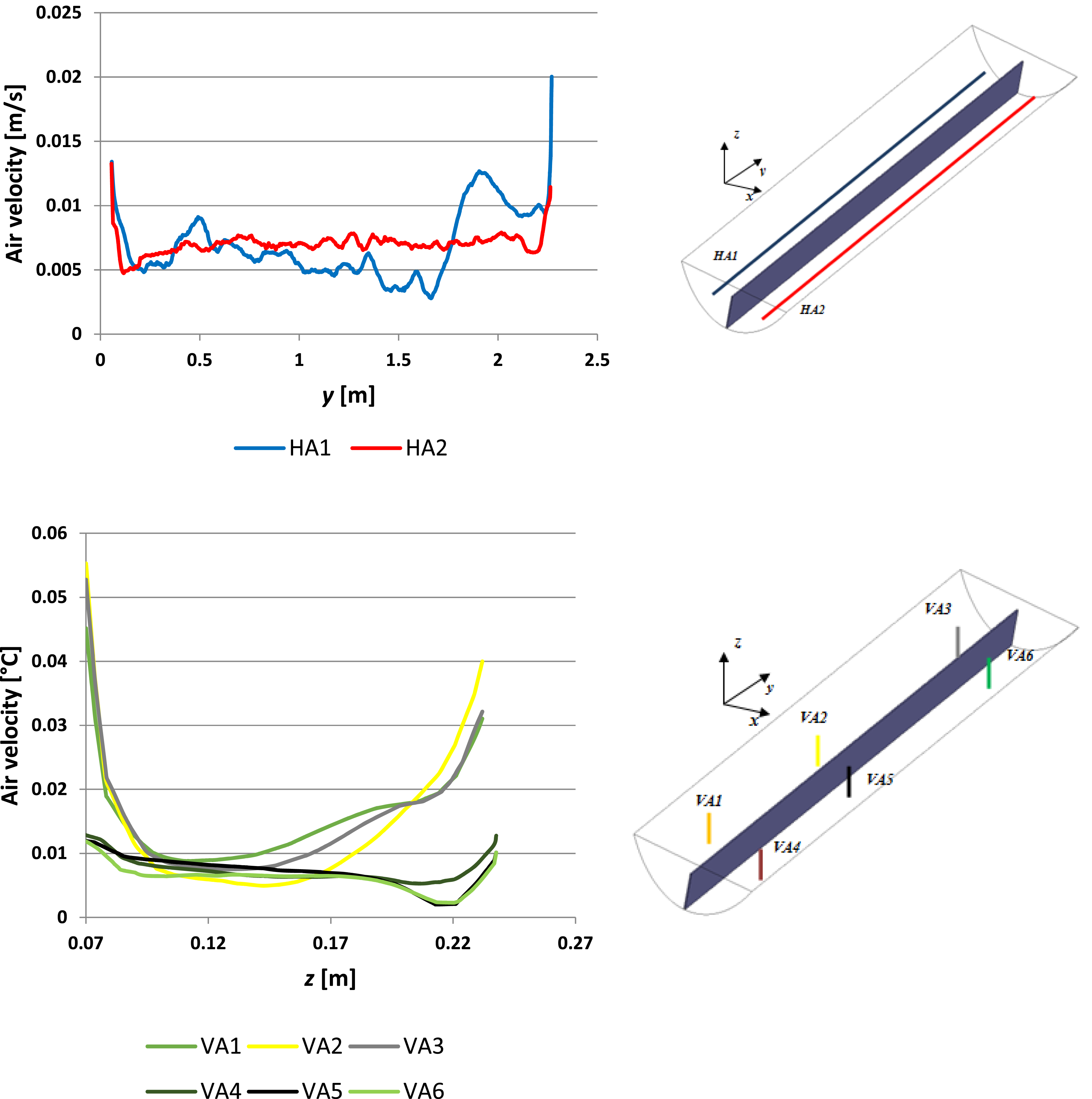
Rather low air velocity magnitude is reported along with horizontal profile HA two i.e. in points that are located below the receiver. Such low airspeeds arise as a result of natural convection which is the only mechanism that is inducing the flow on a closed collector like the one studied in this case. The convection heat transfer in a closed small cavity like the one studied in case 1, aside from radiation heat transfer, is unlikely to contribute alone for a satisfactory cooling of the cells. It is noticeable, though, a greater air velocity variation in z-direction. This is motivated by the also greater speed gradients found in this direction, namely in the region just below the glass and the receiver, as shown in Figure 9.
Calculated and measured temperatures, air velocities and percentage of error for case 1.
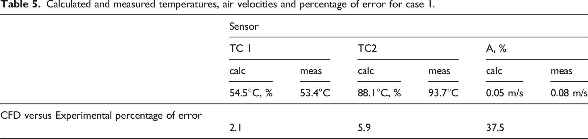
Maximum temperature differences of 5.6°C were found between simulations and experiments, which can be considered acceptable having into consideration the temperature range encountered within the collector at the time it is in operation: 30 to 90°C. Regarding the air velocities data, anemometer A is reading a velocity magnitude of 0.08 m/s, in a point where simulations forecast 0.05 m/s. CFD is, hence, under-predicting the air velocity in this region, for this case. The results, though, can be considered, quite satisfactory, given the uncertainty of the velocity instrumentation of ±0.03 m/s, together with a very low magnitude involved in the measurement of this variable.
Multiple reasons may cause numerical results to diverge from the experimental data. Apart from numerical errors, uncertainty is present in the boundary conditions definitions e.g. heat transfer coefficients, surface emissivity and thermal/physical properties of materials, which may contribute to the observed discrepancies. Furthermore, instrumentation and its accessories like cables, thermocouples and wires are difficult to replicate in the CFD model and may also perturb the flow. This way, the CFD model can be considered validated and suitable to perform the simulations reported below for the investigation of different boundary other than ones described here.
Case 2
Air and cell temperature
Figure 10 details the predicted temperature contours for case 2 in a plane at y = 400 mm. This collector differs from the previous design analysed in the previous section in a way that it explores an alternative for an enhanced cooling of the cells. In this case, the side gables are the only component removed, although the top glass remains installed. All the operating conditions i.e. material properties, ambient temperatures and solar irradiation, used for tests and simulations of case 1, are kept constant. Predicted temperature contours in a plane at y = 400 mm for the case 2.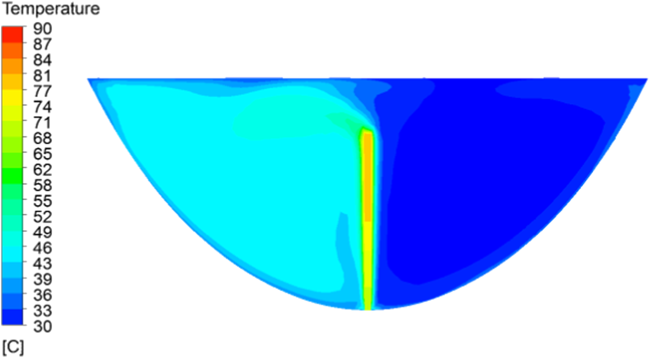
For comparing purposes, the temperature scale used in the discussion in the previous section was the same. Presented data suggest a clear reduction both on air and receiver temperatures, compared to the fully closed collector case. Air almost reaches ambient temperature on the lower part of the collector, whereas approximately 49°C is found on the majority of the zone on the remaining part of the collector. The receiver is working at temperatures ranging between 58°C and 81°C. The absence of the side gables makes the cooling of the receiver much more efficient since it allows mass transfer between the interior of the collector and ambient domains, which greatly contributes to the cell temperature regulation. Figure 11 illustrates the temperature profiles along y and z axis for case 2. Calculated temperature profiles in the air and cells over three and nine lines over y and z directions, respectively, for the case 2.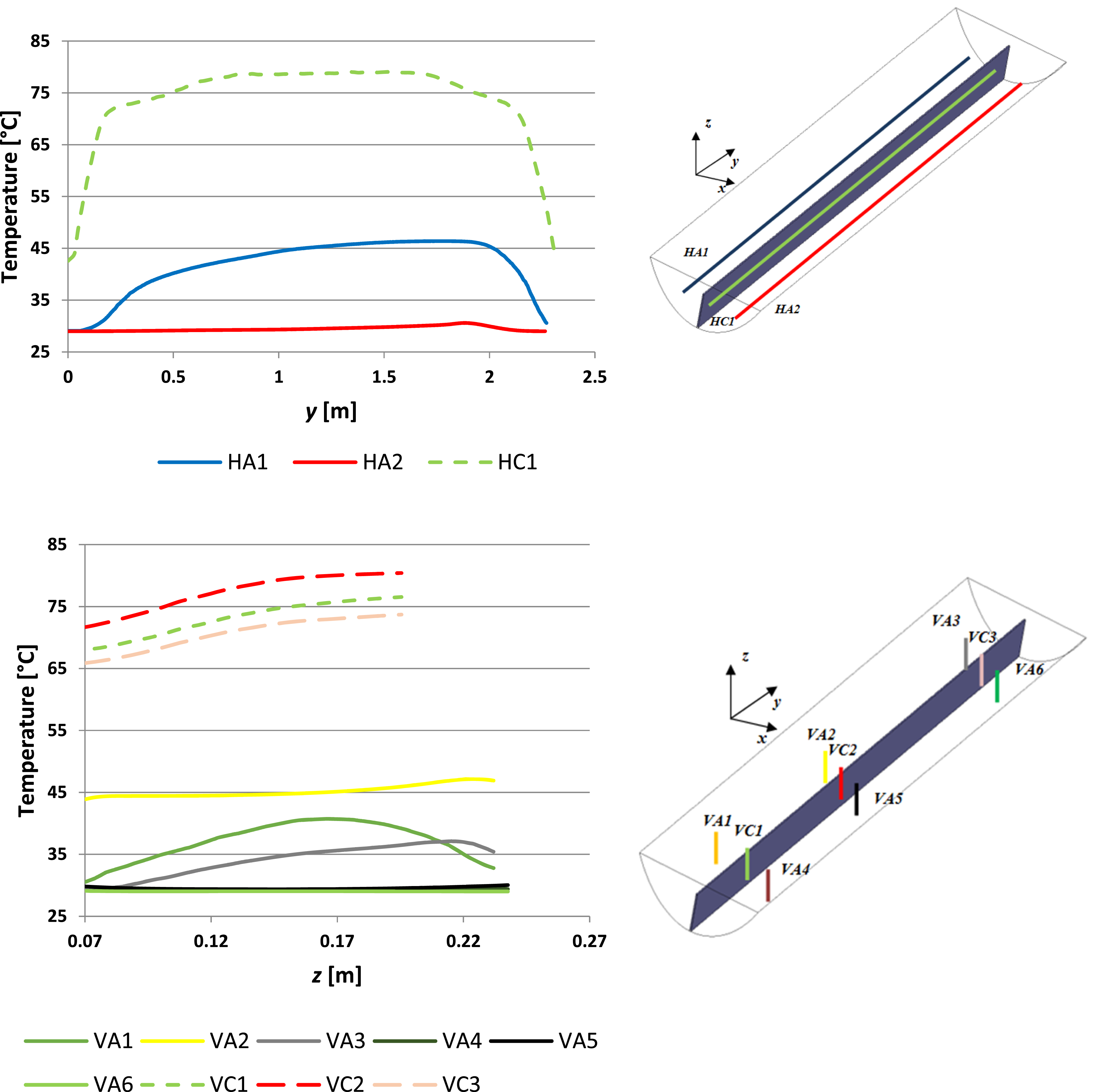
There is a pronounced temperature decrease in both ends of the collector i.e. near the location where the side gables used to be installed. Profile HA2 indicates also that the temperature remains almost constant from y = 0 m to y = 2.25 m which is around 0.6° C above ambient temperature which is much lower than what was reported for case 1, of a closed collector. The vertical temperature profiles i.e. over z direction point to a small thermal stratification in the air in some zones (around line VA2 and VA5), whereas next to the extremities, profiles reveal more pronounced differences with the height of the collector (profiles VA1 and VA3). Regarding the temperature of the cells, a difference of about 10°C is observed between their base and top.
Air velocity
Figure 12 shows the calculated velocity vectors and magnitude contours for case 2. Predicted velocity contours in a plane at y = 400 mm for the case 2.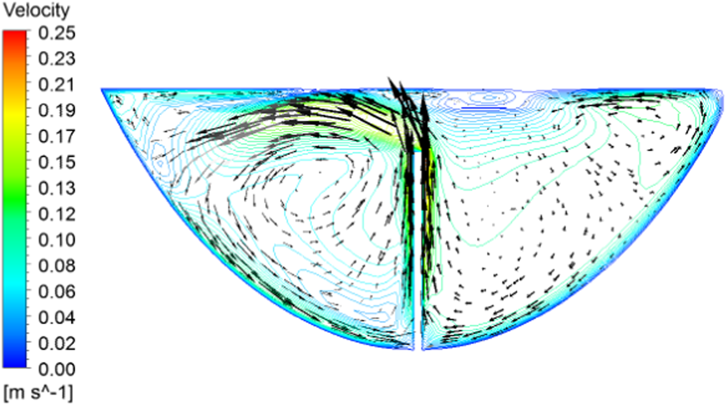
Results indicate the development of a vortex in the upper zone like the one detected in Figure 8 for case 1. In fact, the general pattern of the flow found here, bears resembles the previous case, with particles moving downwards over the walls of the reflector and ascending over the surface of the receiver. This is expected since the latter is the hottest surface of the collector. Higher velocity magnitudes, though, are detected here comparing the two cases. Figure 13 exhibits the calculated air velocity profiles for case 2. Calculated velocity profiles over two and six lines over y and z directions, respectively for the case 2.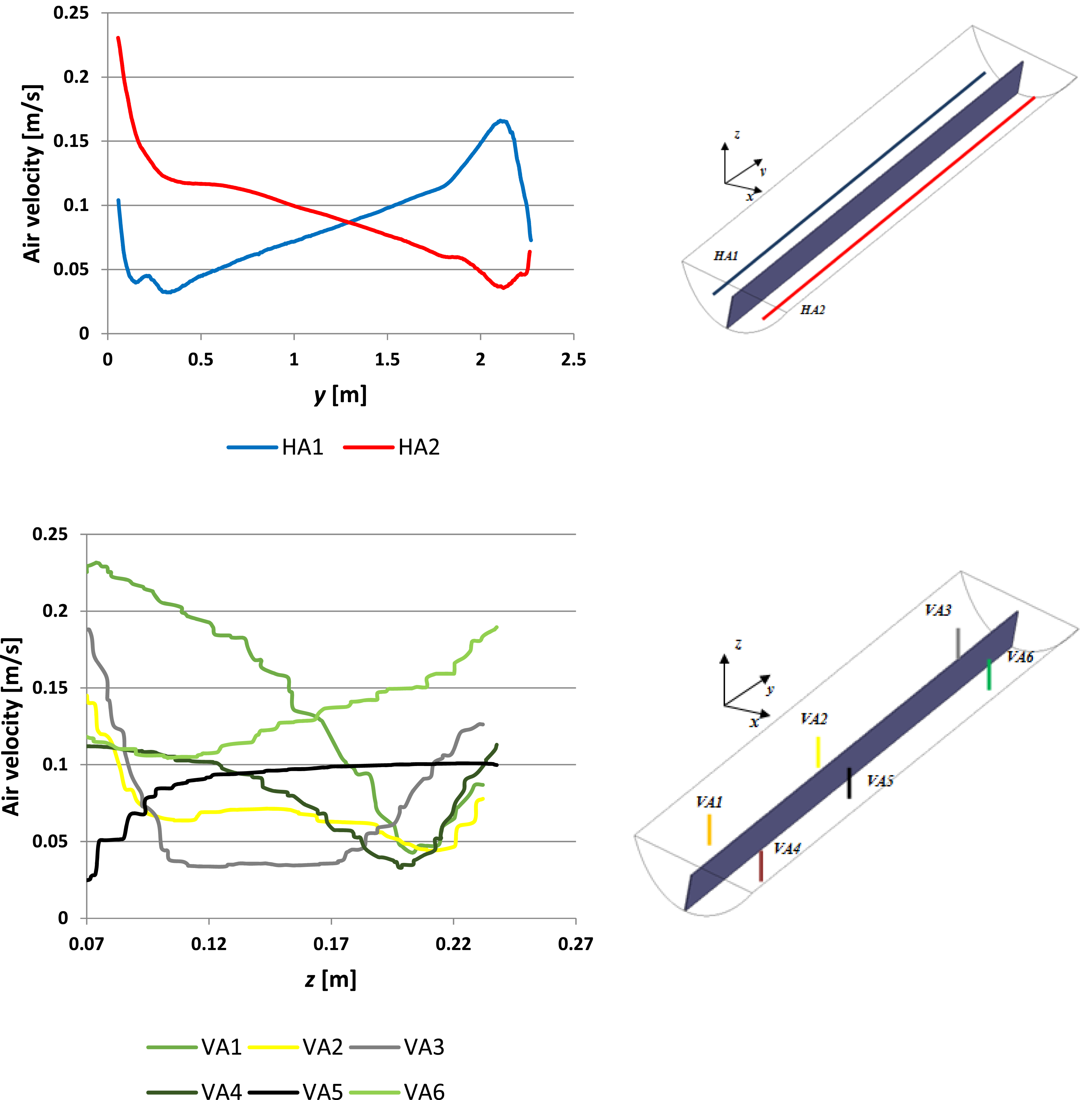
Results show an asymmetric distribution of the velocity towards the y axis. This is because a particular airflow distribution is found in the plane where the opening sections are located. The air enters and leaves the collector when temperature differences take place. As a result, at lower heights, lower temperatures (or higher densities) occur and ambient air is likely to be sucked into the collector, whereas at higher heights this induces an exhaust of hot air flow out of the collector. The vertical profiles in Figure 13 show that in this case an increase in the velocity magnitude up to 5 times higher is expected compared to that found in the simulations for a fully closed collector - case 1. This increase in the air velocity may explain why lower than previous case temperatures are achieved with this solution (already discussed earlier in The Air and cell temperature) once higher convection heat transfer rates are likely to occur. This also demonstrates the ability of the solution proposed to contribute to better dissipation of the heat.
Case 3
Air and cell temperature
As mentioned earlier, a collector with assisted cooling was simulated in order to investigate a presumably more efficient method for the regulation of PV cells temperature than the one suggested in case 2. Boundary conditions were set for the model to reproduce the extraction of air by mechanical means e.g. using a pair of fans. In the field, this can be accomplished simply by opening a couple of circular vents on each lateral gable and then attach a pair of small ventilators to one of the sides. These will pull the hot air out of the collector and, as a result of the depression being generated, cold air is sucked and forced to flow from the exterior all way to the extraction openings, this way helping to cool down the collector.
Two circular openings were, therefore, created in the model used for case 1. This was the only modification carried out in the previously used CFD model besides, obviously, the change in the boundary conditions. For the sake of comparison between the cases, the other variables used in the simulation’s conditions have remained unchanged. The diameter of each opening is 100 mm and they are positioned 75 mm from their center to the surface of the receiver. The velocity adopted in simulations was 5 m/s. This is the velocity achieved by a 100 mm in diameter, typical, domestic line axial impeller with an air flow of 150 m3/h. The velocity profile was assumed to be uniform through the inlet. Figure 14 illustrates the predicted temperature contours in a plane at y = 400 mm for the case 3. Predicted temperature contours in a plane at y = 400 mm for the case 3.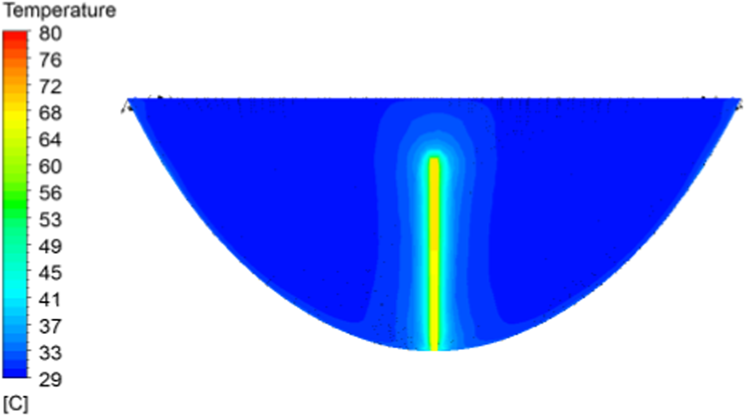
This particular configuration yields quite homogeneous air temperatures along this section, which are equal to ambient temperature at 29°C. While the air around the receiver may increase to approximately 45°C, the receiver still shows a maximum of 68°C. If a comparison between similar strategies has to be made,
21
observed a 15°C reduction in the operating temperature of the cells using fans to cool the backside on a roof-mounted P.V. modules. The introduction of outside air results in an effective way to lower the cell temperature versus a fully closed collector – the maximum temperature found on cells was 88.1°C in case 1 (see Figure 6). Furthermore, a more homogenous spread of the temperature in the receiver is also achieved. This is especially relevant to avoid problems related to thermal expansion often found in this type of concentrating technology. Figure 15 presents the calculated temperature profiles along y and z axis for case 3. Calculated temperature profiles in the air and cells over three and nine lines over y and z directions, respectively, for the case 3.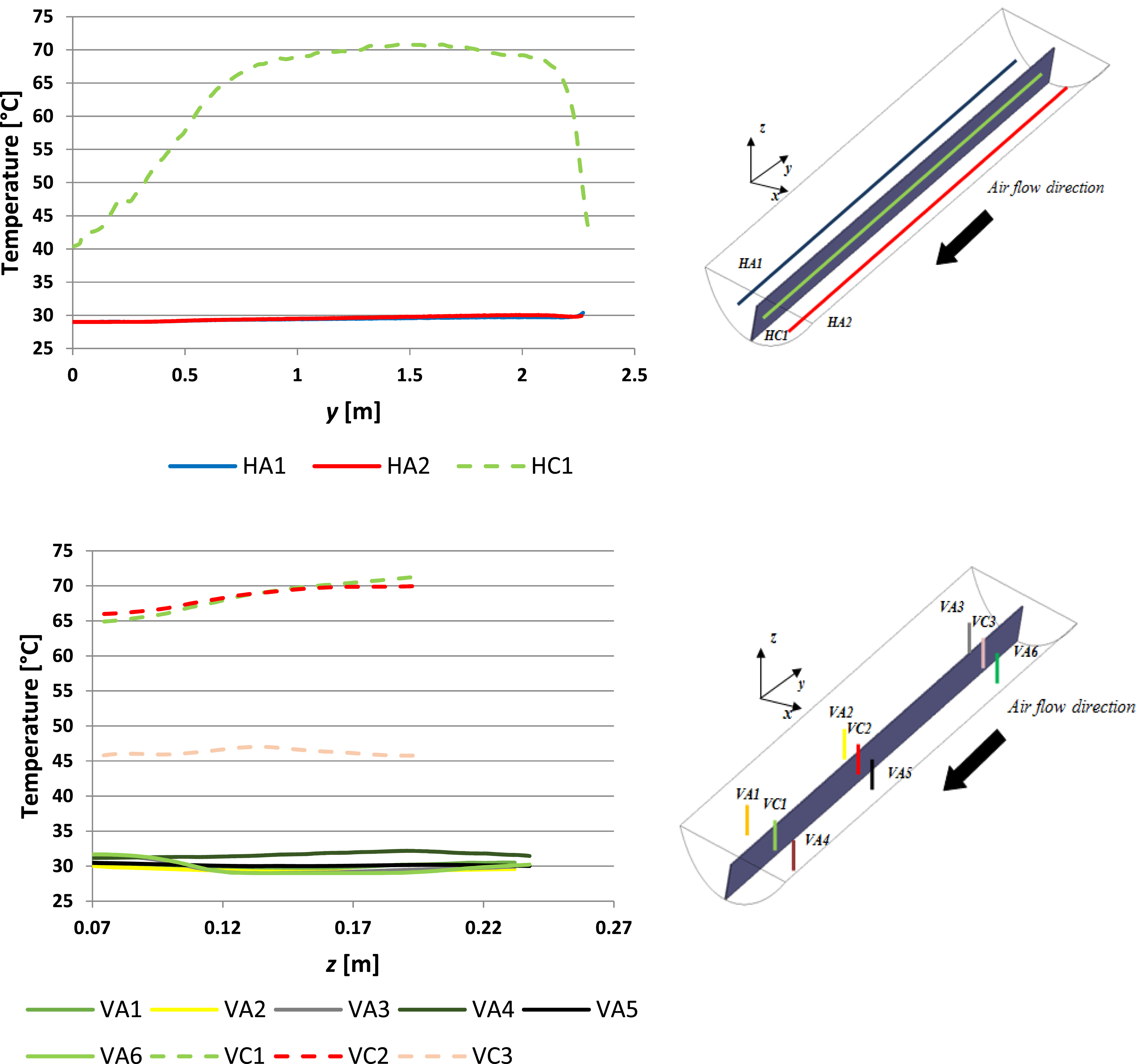
Taking the data from the simulations namely those which show fluid and solid domains temperatures, it is possible to identify a considerable better cooling effect of the cells. However, the profile over the line HC1 shows that this achievement occurs more pronouncedly during the first 0.8 m and that the temperature of the cells remains approximately constant beyond this point.
Air velocity
Figure 16 shows the predicted velocity contours and vectors for the case 3 along normal and longitudinal planes to the air flow direction, respectively. Predicted velocity contours (a) in a plane at y = 400 mm and (b) in a plane at z = 125 mm for the case 3.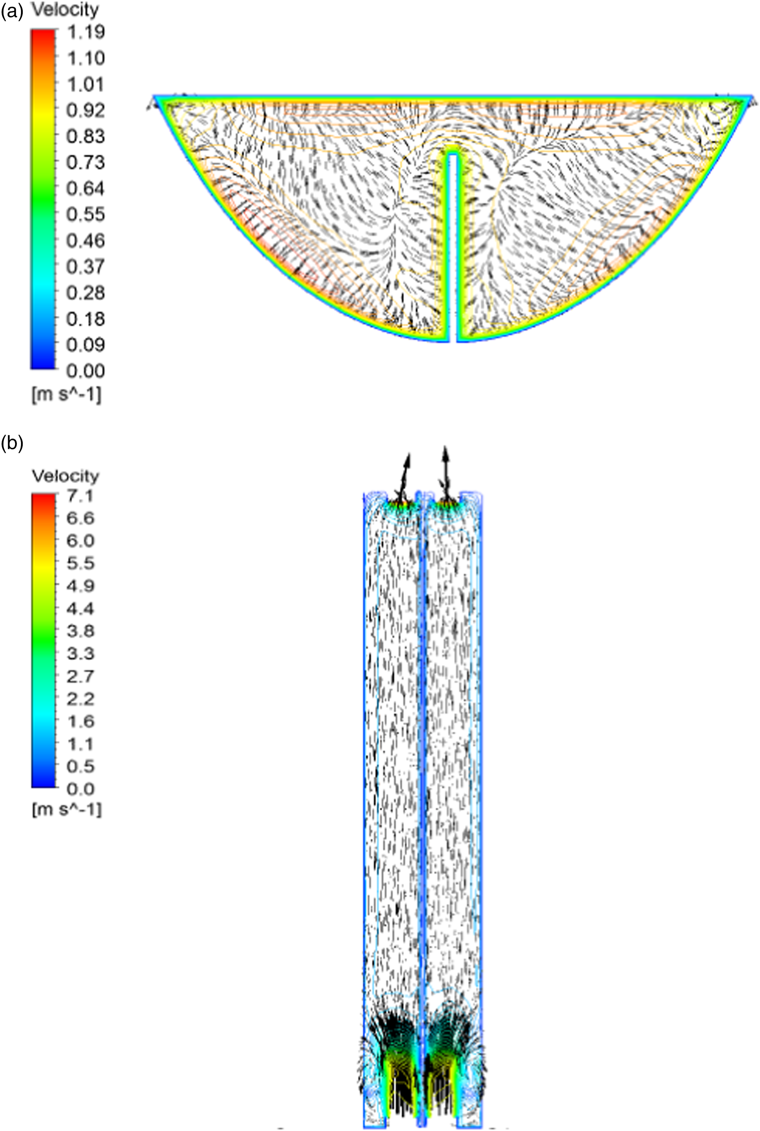
In this arrangement, Figure 16 (a)) points out several differences with the two cases studied before. It shows a ruling direction of the velocity which is mainly pointing to a normal to this section of the collector. This is because although both mechanisms of convection – natural and forced, are present, the latter is showing clearly to be the driving force in this flow. Figure 16 (b)) identifies the predominant direction assumed by the flow and also the abrupt decay on the air velocity after y = 0.25 m. This is an expected behavior, and it is normally found in round jets like the one that appears here, and may explain the uneven cooling of the receiver already reported when the discussion of Figure 15. Figure 17 shows the velocity profiles calculated along the y and z axis for the case 3. Calculated velocity profiles over two and six lines over y and z directions, respectively for the case 3.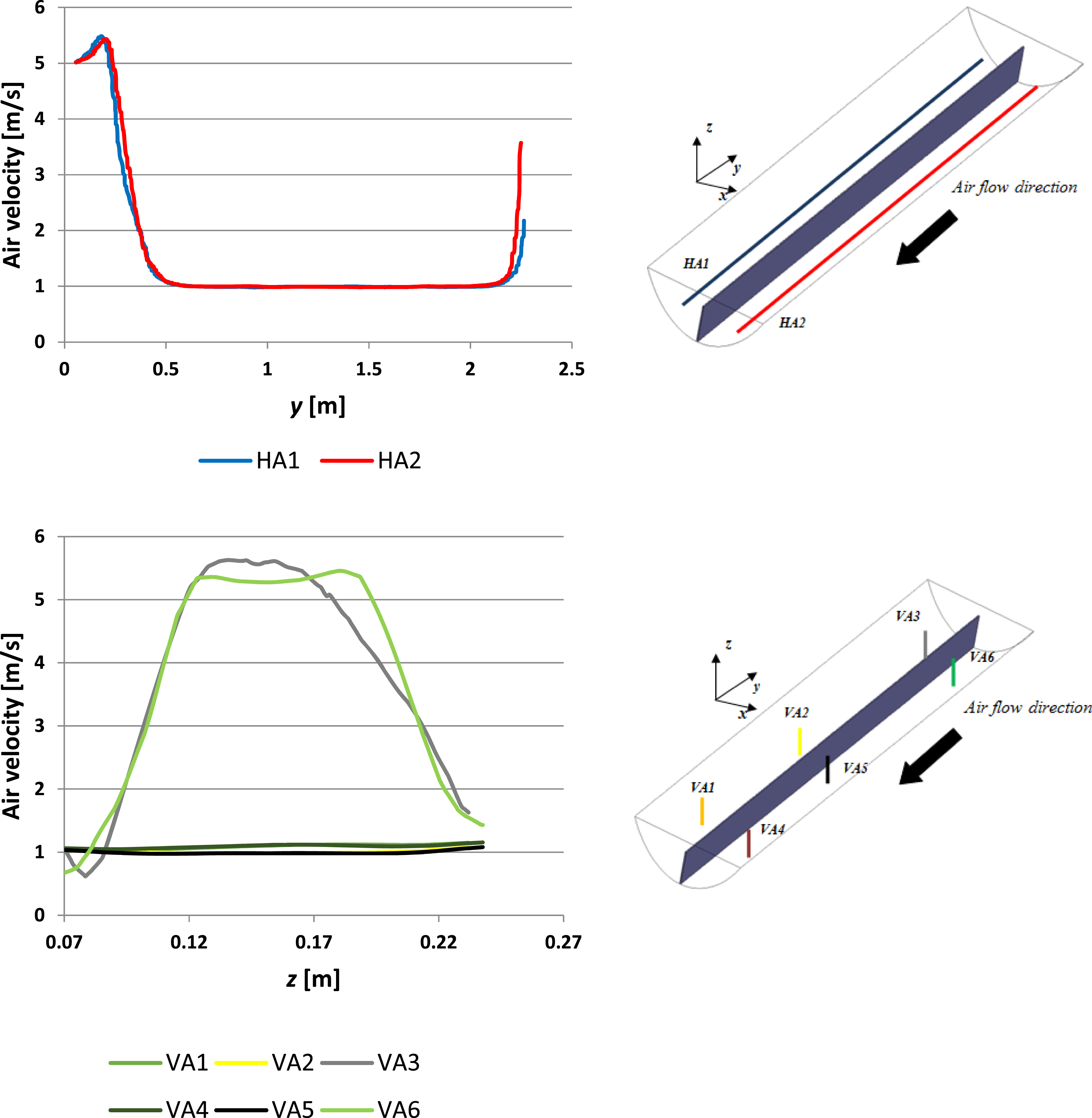
Both charts suggest that among the three cases presented in this study, this particular one is where the highest magnitudes are likely to be encountered. A peak it is also notorious in the air velocity, which happens in y≈0.2 m, followed by a decrease to 1 m/s and that it remains constant just before the end of the cell string. The sudden increase that is taking place in this region is originated from the contraction of the flow ahead of the opening. This is noticed both in curves of the profiles HA1 and HA2 with small differences between them. This fact was confirmed when the analysis of Figure 16 (b)). The vertical profiles (which are normal to the glass surface) VA3 and VA6 show much greater air velocities than the rest, mainly because they are located close to the inlet opening and corroborate what was already discussed for the horizontal profiles.
The calculation of the heat transfer coefficient is far from being a simple task. It is mainly affected by turbulence and the reference temperature chosen in calculation. These variables may explain the difference between the results of the three methods presented previously. In the other hand, its variation along with the position makes the use of a local or an average number a simplification that can lead to significant errors in the analysis. Nevertheless, the CFD model developed in this study has shown to be both a robust and useful tool for thermal analysis in collectors and it allows to explore innovative solutions that increase collector efficiency when converting the sun´s light into electricity.
Conclusion
In the present article, the thermal performance of a Concentrating Photovoltaic collector was studied. Tests were made on an experimental set-up and simulations were carried out on two prototypes of a concentrating collector using bifacial cells. Some conclusions can be drawn about the thermal performance of each configuration studied: (i) The temperature of the cells decreases as the protections are removed from the collector. A reduction of 13.5% is found when comparing case 1, a completely airtight collector, equipped with glass and side covers, with case 2 - without the side gables. (ii) The decrease in the temperature of the air inside the collector box is achieved as a result of the lateral gables being removed and is much more significant than the lowering in PV cells temperature. (iii) As expected, for case 3, the bifacial receiver has a maximum temperature from a length of 1 m to almost 2 m, which shows the high impact of the side covers regarding the receiver temperature distribution, as mechanical ventilation for forced ventilation is applied. (iv) On the other hand, for case 2, the bifacial receiver has a higher and more even distribution of the material temperature than case 3, due to the fact that case 2 applies a natural ventilation method, whereas case 3 applies a forced ventilation method. (v) Compared to natural convection mechanisms, forced convection results in an increased cooling effect when applied to the collector. A reduction of 22.8% was found in the maximum operating cell temperature comparing the case 1 and 3 which leads to higher electrical efficiencies.
Others than circular geometries and locations of the openings used in this study need to be investigated, though, in order to optimize the cooling of the collector. Also, the gain in efficiency by cooling the cells comes with an additional energy cost to power the ventilators. Although net positive, the overall balance should constitute a topic of discussion and deserves to be further investigated.
Footnotes
Acknowledgements
The authors would like to thank Gävle University, the company MG Sustainable Engineering AB and Erasmus + Program for the opportunity given to conduct the experiments that lead to the production of this article.
Declaration of conflicting interests
The author(s) declared no potential conflicts of interest with respect to the research, authorship, and/or publication of this article.
Funding
The author(s) received no financial support for the research, authorship, and/or publication of this article.