Sage Journals: Discover world-class research

Abstract

To better understand the effect of vortex shedding on the nature of the trailing edge shock system during airfoil limit loading a computational fluid dynamic investigation was performed for a transonic turbine airfoil at sublimit, limit and supercritical conditions. Four modeling strategies were employed: steady state RANS, unsteady RANS, DDES, and turbulence model free. The influence of transient modeling approaches on the predicted mass-flow averaged total pressure loss coefficient, mass-flow averaged flow angles, and on the limit loading pressure ratio were found to be insignificant with the exception of the URANS model during critical loading. It was found that the URANS modeling approach failed to predict the transition from near trailing edge dominated vortex formation to base pressure vortex formation resulting in a drastic rise in predicted total pressure loss. Surface isentropic Mach distributions were predicted similarly for all modeling strategies, with the exception of the trailing edge base pressure region and points of shock impingement along the suction surface. A detailed review of the boundary layer states at the trailing edge was performed. It was found that all of the modeling approaches predicted laminar boundary layer profiles along the pressure surface trailing edge and turbulent profiles along the suction surface. The predicted base pressure distributions were also reviewed, showing the base pressure to decrease with increasing pressure ratio. The unsteady simulation approaches consistently predicted lower average surface pressures than the steady state RANS simulations. Qualitative images of the numerical Schlieren contours were presented and reviewed showing large differences in the prediction of vortex shape, size, and subsequent shock influence.

Keywords

Airfoil limit loading computational fluid dynamics modeling turbine airfoil development

Introduction

To stay competitive within the gas turbine community, turbine aero designers strive to maximize the total work output of each turbine stage through a combination of pressure ratio increase and airfoil design improvements. Although the higher power target could be achieved by increasing mass flow rate, the corresponding increase in turbine annulus area would result in structural limitations due to longer blades which cause increased strain on the blade root as well as amplified flutter and rotor dynamic excitation. An alternative path to achieving higher power output is to maximize the loading of each turbine stage through increased pressure ratio, but this may also lead to airfoil limit loading and high aerodynamic losses.

The limit loading condition was first documented by Hauser and Plohr in a National Advisory Committee for Aeronautics (NACA) Research Memorandum in the 1950s.^1,2 They identified the blade outlet metal angle as the dominant geometric parameter to influence limit loading behavior. Following their review, numerous studies set out to provide a numerical method to predict the onset of airfoil limit loading.^3–5 These investigations proved to predict the required limit loading pressure ratio reasonably well, but they failed to provide detailed flow characteristics.⁵

Recently computational fluid dynamics (CFD) has been used to provide a more in-depth analysis of the flow dynamics within a gas turbine blade passage giving designers a better understanding of the limit loading condition. Chen preformed the first detailed CFD investigation for a range of pressure ratios from sub-critical to supercritical loading.⁵ Quantitative data of mean-flow Mach number, flow angle, blade forces, mass flux and total pressure loss coefficient were determined and presented alongside contours of total pressure and flow streamlines. It was shown, contrary to prior studies, that CFD provided a sufficient tool for predicting the onset of airfoil limit loading. Chen also provided a formal definition of the limit-loading condition based on channel flow theory. Expanding on this work, Owen investigated the effects of off-design inflow conditions for four different transonic turbine airfoils over a similar range of pressure ratios by varying inflow boundary conditions: incidence from ±20°, turbulence intensity from 5 to 20% and turbulent length scale from 1 to 100% of the airfoil pitch.⁶ Similar to previous experimental work, it was shown that the limit loading pressure ratio and the mass-flow averaged outlet flow angle were strongly correlated with the airfoil outlet metal angle. The influence of inflow conditions on the exit flow profile was found to be minimal with the exception of the mass-flow averaged total pressure loss coefficient. Results showed that variation of incidence affected the total pressure loss coefficient of each airfoil differently, whereas increasing turbulence level resulted in higher loss coefficients for all airfoils.

These studies also showed that CFD has the ability to accurately predict the onset of limit loading as well as to provide increased understanding into the steady-state flow picture. However, there has yet to be an investigation documenting the effects of transient phenomena on the limit loading state. This paper provides a review of common unsteady simulation approaches, allowing for an assessment of the influence of transient phenomena on airfoil performance as well as an analysis of the capabilities and limitations of each modeling approach.

Shown in Figure 1 is a visual description of the terminology used to describe the stages of airfoil loading from critical to supercritical conditions. The set of images along the top show a simplified representation of the trailing edge shock structure for a transonic turbine airfoil, while the bottom provides a realistic contrast of numerical Schlieren RANS CFD predictions for the airfoil studied in this paper.

Figure 1.

Limit loading: terminology.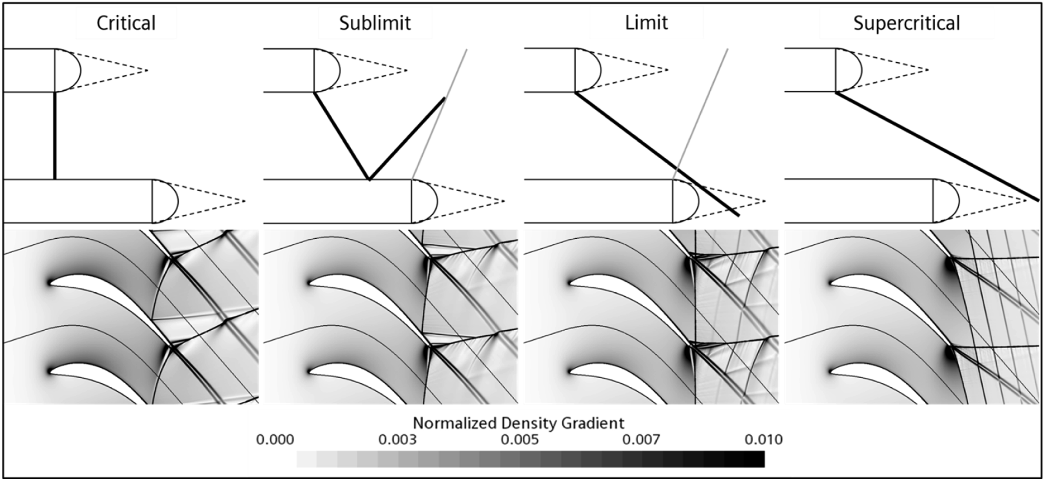

The left most image, characterized by a strong Trailing Edge Pressure Side Shock (TEPSS) normal to the airfoil surface, describes the critical loading condition. At this point the pressure ratio across the airfoil results in choking of the flow upstream of the throat. As the pressure ratio is increased the TEPSS becomes oblique due to the Prandtl-Meyer expansion near the trailing edge. The TEPSS impinges on the adjacent airfoil suction surface and reflects downstream, ultimately coalescing with the weaker Trailing Edge Suction Side Shock (TESSS) and further propagating downstream towards the wake. It should be noted that for any turbine airfoil there is a range of pressure ratios from critical to limit loading, here defined as the sublimit loading range. The size of this pressure ratio range has been discussed by Owen and shown to be dependent on the airfoil geometry, specifically the airfoil stagger angle and trailing edge blockage ratio.⁶ Further increase of the pressure ratio causes the TEPSS to obtain sufficient flow turning to completely miss the surface of the adjacent airfoil, moving into the base pressure region downstream of the trailing edge. This is the point of maximum loading and is defined as the limit loading condition. Super critical loading is the fourth and final loading condition, shown as the right most set of images in Figure 1. Here a strong oblique TEPSS is produced that propagates downstream of the base pressure region of the adjacent airfoil and into the flow passage, causing the entire domain to become choked.

The objectives of this work are to (1) identify the effects of vortex shedding on the nature of the trailing edge shock system during airfoil limit loading, specifically on the impact to the base pressure distribution, upstream boundary layer state and downstream total pressure loss, and (2) document an assessment of the ability of each modeling approach to aid in the decisions of turbine aero designers. All simulations were preformed using a commercial finite volume code, Star-CCM+. Quantitative data of mass-flow averaged total pressure loss coefficient, mass-flow averaged flow angles, surface isentropic Mach number distributions, surface base pressure distributions, trailing edge boundary layer velocity distributions and vortex shedding frequencies are presented alongside flow visualizations of numerical Schlieren images to provide insight into the influence of transience on airfoil limit loading.

The authors would like to highlight that the work described in this paper formed part of a PhD dissertation at the University of North Carolina at Charlotte.⁷

Numerical methods

Airfoil description

Two transonic turbine airfoils, shown in Figure 2 were used in this study: the first from the thesis of Sooriyakumaran at Carleton University in Ottawa, Canada,⁸ and the second from the work of Sieverding at the European Research Project BRITE/EURAM CT96-0143 on “Turbulence Modeling of Unsteady Flows in Axial Turbines”.⁹ The profile adapted from Sooriyakumaran is the main focus of this paper; however, the airfoil profile from Sieverding was also analyzed to ensure adequate validation of the transient nature of the flow dynamics around the trailing edge. Table 1 shows the relevant geometric parameters for each profile. As shown, the airfoil from Sieverding’s study has a much larger trailing edge thickness as well as higher unguided turning and stagger angle than the profile from Sooriyakumaran; however, the pitch-to-chord ratios for both profiles are similar. The airfoil testing aspect ratio for the results for the wind tunnel testing performed by Sooriyakumaran were over 1.5 to ensure end-wall effects could be ignored and the midspan flow assumed to be fully two-dimensional.¹⁰

Figure 2.

Airfoil normalized profiles.

Table 1.

Airfoil geometric characteristics.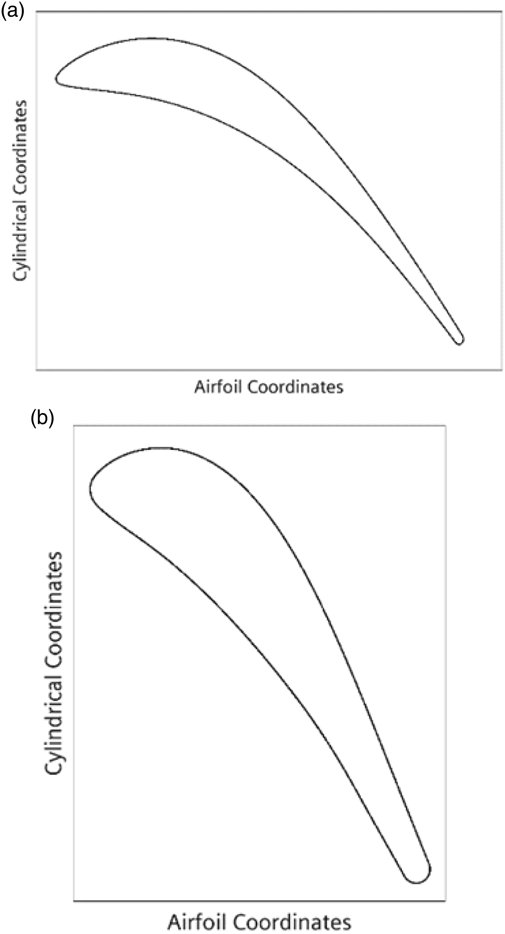

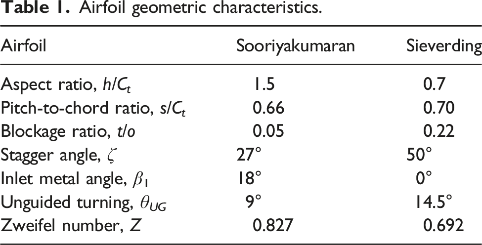
Airfoil	Sooriyakumaran	Sieverding
Aspect ratio, h/C_t	1.5	0.7
Pitch-to-chord ratio, s/C_t	0.66	0.70
Blockage ratio, t/o	0.05	0.22
Stagger angle, ζ	27°	50°
Inlet metal angle, β₁	18°	0°
Unguided turning, θ_UG	9°	14.5°
Zweifel number, Z	0.827	0.692

Figure 3 shows the computational domain used for this study. The inlet plane was positioned 1.5 axial chord lengths upstream of the airfoil leading edge to ensure uniform and fully developed flow. The extent of the outlet boundary, positioned seven axial chord lengths downstream of the trailing edge, was chosen specifically for the limit and supercritical loading conditions to ensure numerical reflections did not influence predictions near the evaluation area.¹¹ The evaluation plane is taken to replicate the experiment used for validation and is positioned 1.5 axial chord lengths downstream of the airfoil leading edge. The top and bottom surfaces located a half pitch above and below the airfoil surface were periodic with a one-to-one mesh connectivity. Similarly, the positive and negative spanwise planes used for 3D predictions were periodic with a total thickness of 10% of the airfoil chord and one-to-one connectivity.

Figure 3.

Computational domain and grid.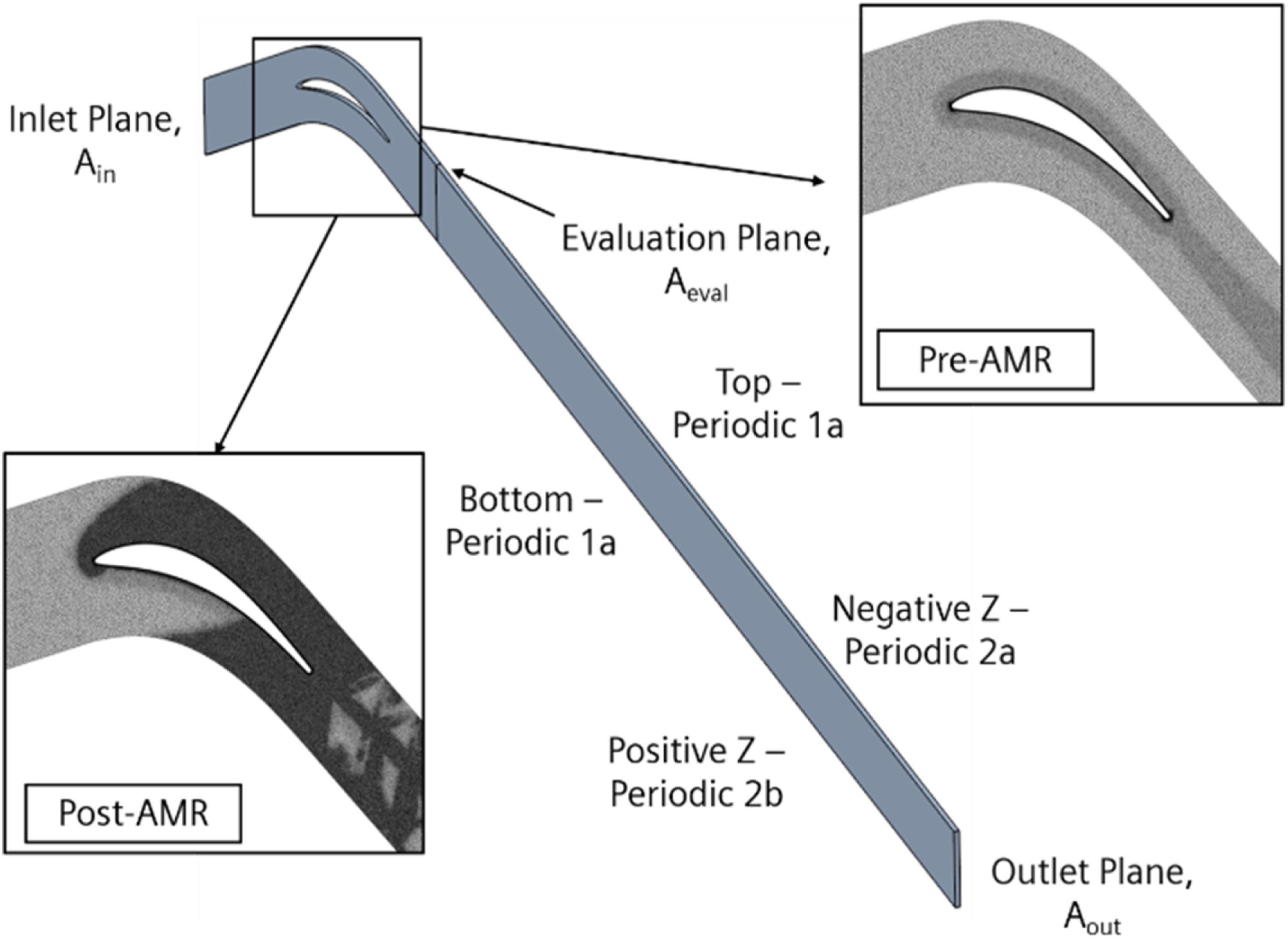

Boundary and initial conditions

Boundary conditions used were set to replicate the experimental conditions of Sooriyakumaran.⁸ The inlet boundary was prescribed a constant total pressure and total temperature, the outlet boundary an average static pressure, the top and bottom along with the positive and negative spanwise extents were set as periodic, and the airfoil surface a smooth, no-slip adiabatic wall. Incidence angle was set to 14°, and inlet turbulence intensity and length scale were set to 4% and 10% of airfoil pitch, respectively. Although uniform artificial inlet turbulence is unlikely in actual turbine engines; the authors choose this approach to ensure that an analogous comparison of downstream modeling approaches could be made, specifically around the trailing edge where shocks are most prevalent at these conditions. The development of true inflow turbulence is considered outside the scope of this paper and will be considered in future work. Outlet average static pressure was adjusted depending on the desired inlet-total to outlet-static pressure ratio. Reynolds number based on the velocity at the evaluation plane and the true chord was Re_c ∼ 1.0 × 10⁶.

It should be noted that although the simulations were setup to replicate the experimental conditions of Sooriyakumaran, not all exact physical conditions can be precisely reproduced. The facility in Ottawa, Canada is a blow-down configuration, and can sustain stable transonic flow for up to 60 seconds. Both Reynolds number and exit Mach number can be varied independently due to an ejector-diffuser assembly.¹⁰ The cooled, dry air is discharged through a wire mesh that generates a known turbulence characteristic and is then directed through the test section. For a detailed description of the experimental facility, an interested reader is referred to either the work of Sooriyakumaran⁸ or Taremi.¹²

A few key differences between the experiment and CFD are listed next. First, the dimensions of the airfoils as well as the working fluid properties have been scaled from engine conditions to appropriate environments for the experimental facility. This is not of concern as the flow Reynolds number was used to match the conditions between simulation and experiment. Second the simulations assume a single midspan blade profile, which is certainly not the case in reality. However, a previous study was performed by Corriveau¹⁰ that showed that an aspect ratio, h/c, of 1.5 is sufficient to allow for a region of essentially two-dimensional flow at the midspan. Lastly, the blades used in the experiment were manufactured using a direct metal laser sintering rapid prototyping process. This additive process was shown to result in a surface roughness of about 10 um, which was not accounted for in the simulations.

The inlet conditions were used to initialize the RANS simulations. However, it should be noted that these simulations employed grid sequencing, so the domain initialization did not significantly influence the convergence rate. Each transient modeling approach was initialized with the respective RANS solution. For example, the URANS, DDES and model free simulations for the critical loading condition were initialized using the RANS converged critical loading solution. A detailed description of the grid sequencing process has been documented by Owen.¹¹

Modeling strategies

Although it is well known that the flow within a turbine blade passage is intrinsically unsteady due to vortex formation around the trailing edge, RANS modeling is the most extensively used simulation method in the gas turbine industry due to lower computational cost.¹³ The unsteady RANS (URANS) modeling approach provides an improvement to the RANS method by stepping the solution in time to capture vortex formation and other transient phenomena with the smallest amount of increased computational effort. A further improvement in modeling capability is the Detached Eddy Simulation (DES) approach which combines URANS and Large Eddy Simulation (LES) strategies.¹⁴

As mentioned, DES is a hybrid modeling approach that uses a RANS solution within the boundary layer and irrotational flow regions while the detached and freestream flow areas are solved using a modified LES. The LES methodology used is dependent on the specific DES model; here the SST k-omega formulation, obtained by modifying the dissipation term in the transport equation for turbulent kinetic energy, was employed to capture the unsteady separated regions. The delayed DES formulation (DDES) was used to enhance the ability of the model to distinguish between the LES and RANS regions.¹⁴

Lastly, to avoid the empirical nature of the turbulence formulations as well as to ensure simulation fidelity, we tried to solve the flow field using an approach which does not rely on any turbulence modeling approaches. This methodology was similar to a direct numerical simulation approach; however, the simulation domain was kept as two-dimensional. Therefore, the authors have termed this as a pseudo-DNS or model free strategy. Using the results from the URANS simulation the Kolmogorov and Taylor length scales were estimated to be of the order 10⁻⁵ and 10⁻⁴ m respectively. Using these estimates it was determined that the average grid size was roughly half the Taylor length scale and roughly 10 times the Kolmogorov length scale. This was determined to be sufficient based on previous numerical investigations.^15,16

All simulations employed a coupled, implicit compressible algorithm to solve the equations for mass, momentum, and energy. Discretization was second order for the source and diffusion terms for all methods except DDES, which was a hybrid second-order upwind/bounded central-differencing scheme. All models used a second-order upwind scheme for calculation of the convection terms for the momentum and turbulence equations. The inviscid, convective fluxes were calculated using Liou’s AUSM+ flux-vector splitting scheme.¹⁷ The Algebraic Multi-Grid (AMG) linear solver with a V-cycle, Gauss-Seidel relaxation scheme and bi-conjugate gradient stabilizer acceleration method were employed.¹⁸

Convergence criterion and time step

All precursor RANS solutions were run until the flow had reached full convergence such that the normalized residuals of all transport quantities were steady and dropped to four orders of magnitude; in addition, the local total pressure loss coefficient did not show fluctuations over ±0.0001 for 1500 iterations which typically occurred around 3500 iterations.

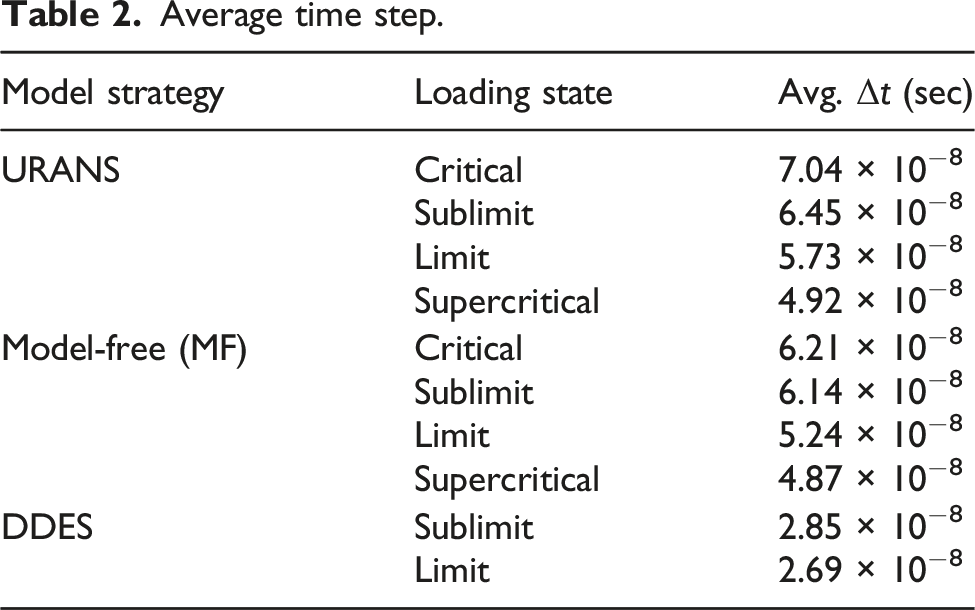
To ensure minimal influence of numerical errors as well as to improve the precision and total run-time of each transient simulation, an adaptive time stepping algorithm was used for each transient simulation. The adaptive time-stepping algorithm adjusts the time-step automatically during the run to obtain a user specified temporal resolution throughout the domain.

The local time-step (Δτ) is computed considering both the Courant number and the Von Neumann stability condition, equation shown below: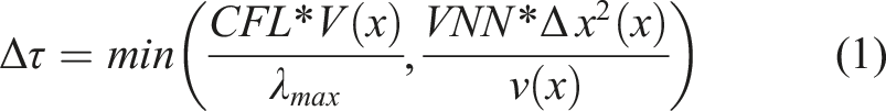

Δ τ = \min (\frac{C F L * V (x)}{λ_{\max}}, \frac{V N N * Δ x^{2} (x)}{ν (x)})

(1)

Here CFL is the user-specified Courant number (dimensionless), V is the cell volume (m³), VNN is the Von Neumann number (VNN = 1), Δx is a characteristic cell length scale (m) and ν is kinematic viscosity (m²/s). λ_max is the maximum eigenvalue of the system as follows:

λ_{\max} = | u \cdot a | + c | a |

(2)

where u is velocity and c the speed of sound.¹⁸

Here an upper limit to the convective CFL number of 0.9 was selected as the criterion to determine the solution time step. Table 2 shows a summary of the mean time-step sizes for each simulation. The required time step to maintain sufficient temporal accuracy is dependent both on the loading condition and modeling strategy employed. The time step size was found to be in the range of 2.6 × 10⁻⁸ to 7.0 × 10⁻⁸ seconds.

Table 2.

Average time step.

Model strategy	Loading state	Avg. Δt (sec)
URANS	Critical	7.04 × 10⁻⁸
	Sublimit	6.45 × 10⁻⁸
	Limit	5.73 × 10⁻⁸
	Supercritical	4.92 × 10⁻⁸
Model-free (MF)	Critical	6.21 × 10⁻⁸
	Sublimit	6.14 × 10⁻⁸
	Limit	5.24 × 10⁻⁸
	Supercritical	4.87 × 10⁻⁸
DDES	Sublimit	2.85 × 10⁻⁸
DDES	Limit	2.69 × 10⁻⁸

Grid description and convergence

As previously mentioned all transient simulations were initialized using a RANS solution. The grid employed for each RANS simulation was generated through an adaptive griding internal algorithm detailed next.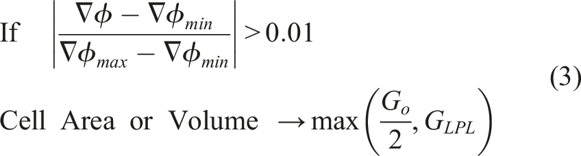

\begin{array}{l} If | \frac{\nabla ϕ - \nabla ϕ_{\min}}{\nabla ϕ_{\max} - \nabla ϕ_{\min}} | > 0.01 \\ Cell Area or Volume \to \max (\frac{G_{o}}{2}, G_{L P L}) \end{array}

(3)

Equation (3) shows the governing process of the adaptive mesh refinement scheme. Here ϕ denotes the scalar quantity of interest (absolute total pressure, total temperature, density, turbulent kinetic energy, turbulent eddy viscosity and the specific dissipation rate of turbulence), G_o the original cell area or cell volume prior to adaptation, and G_LPL is the area or volume of the last prism layer. This was used as the limiter of refinement to ensure a one-to-one ratio between the prism layers and the core grid.

As shown previously,¹¹ the adapted grid algorithm proved robust in capturing the blade loading of four different transonic turbine airfoils at sublimit loading conditions, proving the ability to accurately capture the trailing edge shock system and the subsequent influence on the adjacent airfoil suction side boundary layer. Figure 4 shows an example of the grid density evolution throughout the AMR process.

Figure 4.

Adaptive mesh refinement - example.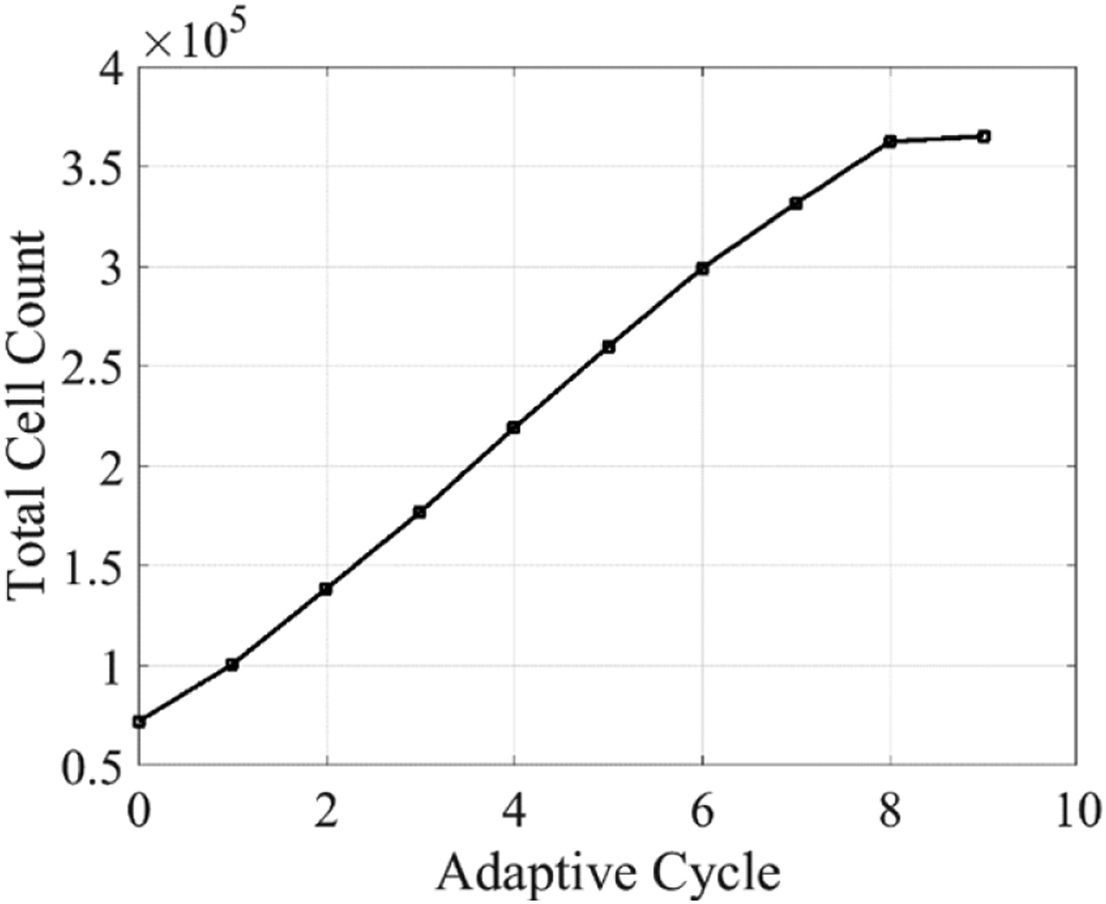

Each simulation began with a baseline mesh of roughly 70,000 elements. The core grid comprised unstructured, polyhedral elements with prismatic layers along the airfoil surface. The distribution of prisms normal to the airfoil remained constant with 40 layers, a hyperbolic growth rate, a near wall thickness achieving a max y+ less than 0.5, and a total thickness equal to 40% of the trailing edge thickness. It should be noted that the distribution along the tangential direction of the airfoil surface was changed with increasing refinement to maintain an aspect ratio of less than two. Nine AMR cycles were used for each RANS simulation, and additional AMR cycles only proved to increase computational resources unnecessarily as the increase in number of elements was less than 1%.

Although this grid methodology provided a grid independent solution for the RANS simulation approach there was no guarantee that it would suffice for the other models. Therefore, an additional grid independent study was performed for each loading condition and transient modeling strategy. Using the adapted mesh from the RANS solution as a baseline, the grid was isotropically refined by 50 and 25%, roughly doubling the total cell count in each case.

Figure 5 illustrates the differences in downstream predicted total pressure loss for each grid level. As can be seen, the change in total pressure loss distribution is minimal between grid refinements, producing a change in mixed-out total pressure loss coefficient of less than 2%. It should be noted that a grid verification procedure was applied to each loading condition for each transient strategy; the image below shows an example. As there was no significant improvement in using the refined grids the adapted grid of the RANS solution was used for each transient simulation.

Figure 5.

Mesh convergence example - downstream total pressure loss distributions - limit loading. (a) URANS, (b) MF, (c) DDES.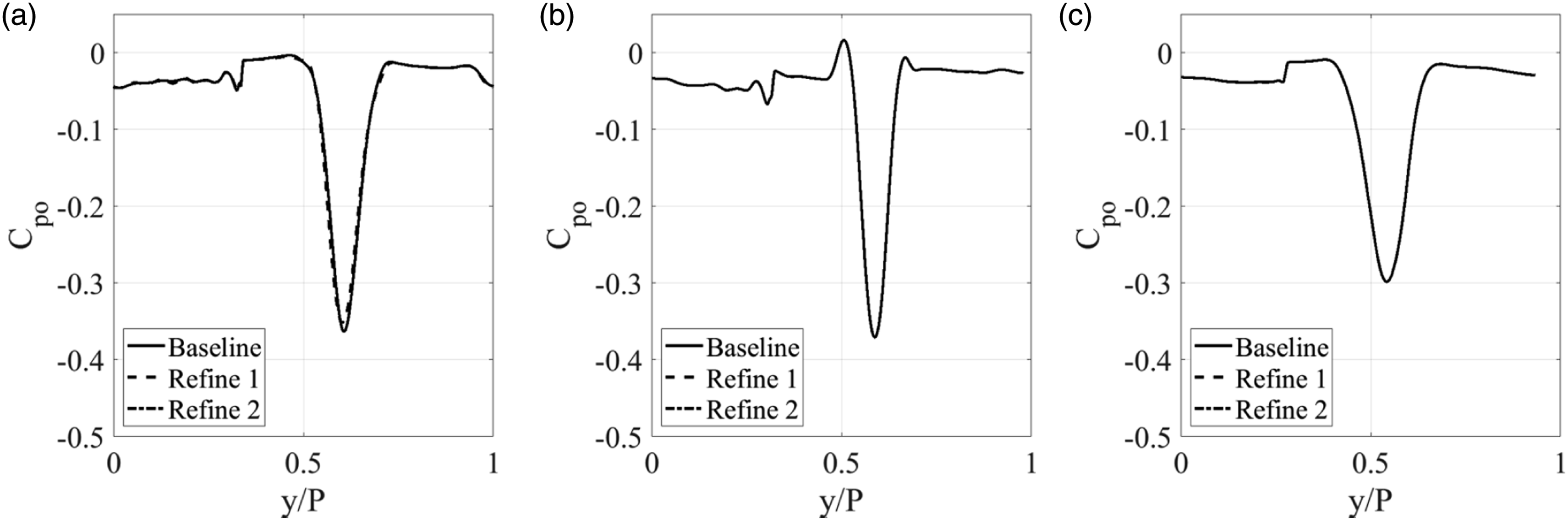

2D/3D RANS and URANS comparison

Prior to the main results section, the authors would like to highlight the differences between 2D and 3D RANS and URANS simulations. Given that the computational domain is modeled as periodic in the spanwise direction, the flow is expected to be similar for both 2D and 3D approaches. Figure 6 shows the surface isentropic Mach number distribution as well as the downstream pitch-wise total pressure loss distribution for both 2D and 3D simulations. Solid lines are the RANS predictions, dashed lines are the URANS predictions, and solid black squares are experimental data taken from the work of Sooriyakumaran.

Figure 6.

2D and 3D domain comparison example - RANS and URANS - sublimit loading (PR = 2.25). (a) Downstream total pressure loss, (b) Blade loading.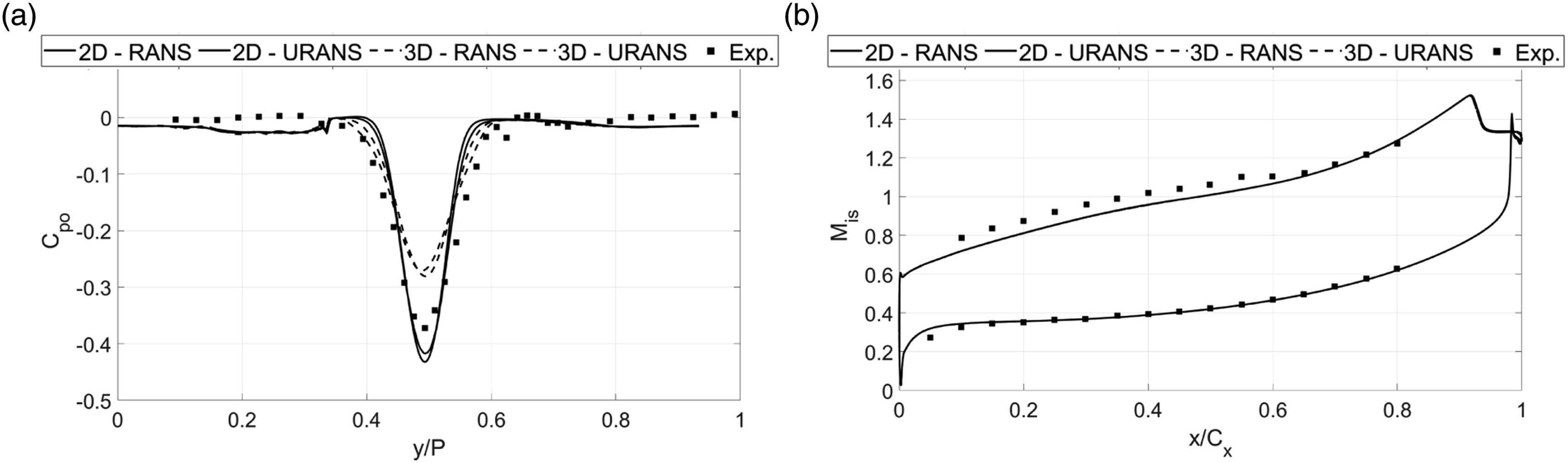

Looking at the blade loading distribution, it is clear there is no noticeable difference between 2D and 3D simulations. On the pressure side the flow accelerates consistently until the trailing edge expansion while the suction side shows a slight deceleration at the leading edge followed by nearly constant acceleration until the point of shock impingement. Following the shock/boundary layer interaction there is a period of nearly constant pressure until the trailing edge. This flow pattern is consistent between modeling domains.

Similarly, the downstream total pressure loss distribution shows only minor deviations between 2D and 3D approaches. The RANS simulations predict a significantly higher loss distribution in the middle of the wake with smaller width compared to URANS. As no major differences were seen between 2D and 3D results for both RANS and URANS modeling approaches, the remainder of the paper will only include the results from the 2D simulations.

Results and discussion

Validation

As previously mentioned, two transonic turbine airfoils were used for numerical validation. Both airfoil geometries have been previously described and are shown in Figure 2. The total inlet to outlet static pressure ratio used by Sooriyakumaran was 2.25, a pressure ratio within the sublimit loading range, corresponding to an isentropic exit Mach number of 1.15 and for the profile used by Sieverding PR = 1.5, a subcritical loading condition corresponding to an isentropic exit Mach number of 0.79.

Figure 7 illustrates the predicted airfoil surface isentropic Mach number distribution for each profile compared to their respective experimental data. Extracted test information is shown as solid black squares while all simulation results are shown as various line distributions; RANS - solid lines, URANS - dashed lines, model free - dotted lines and DDES - dashed dotted lines.

Figure 7.

Validation - comparison to experimental data - blade loadings. (a) Sooriyakumaran - sublimit loading (PR = 2.25), (b) Sieverding - subcritical loading (PR = 1.5).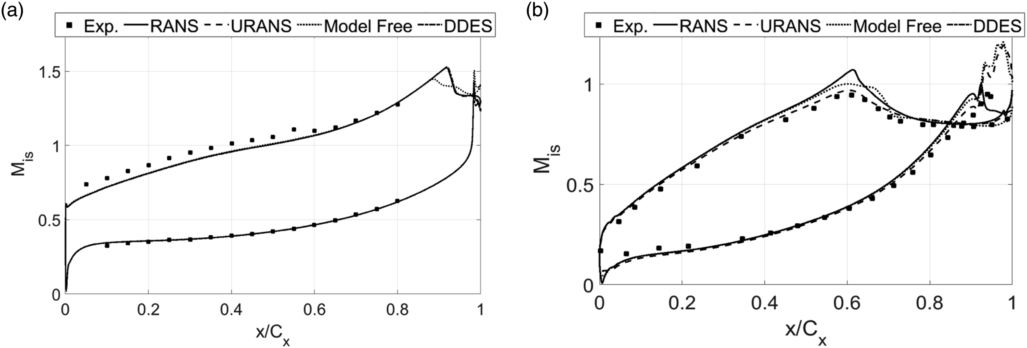

Overall distributions are predicted well for both profiles and loading conditions. Results for the profile taken from the work of Sooriyakumaran show nearly identical predictive capability for the full pressure surface as well as the majority of the suction surface. Differences arise along the suction surface at roughly 0.9 axial chord lengths (C_ax) aft of the airfoil leading edge, at which point the model free approach predicts a smearing of the shock impact on the suction surface boundary layer. This is a product of an oscillatory effect caused by the unsteady vortex shedding at the airfoil trailing edge, and additional details will be provided. Similarly, the predicted results for the profile used by Sieverding agree quite will with the experimental test data for the majority of the airfoil surface. Discrepancies between modeling approaches arise at the point of shock impingement along the suction surface similar to what is observed for the profile used by Sooriyakumaran. This is believed to be primarily a product of the unsteady propagation of vortices near the trailing edge.

Next a look at the downstream total pressure loss distribution for the profile used by Sooriyakumaran as well as the base pressure distribution of the profile used by Sieverding are presented in Figure 8. Focusing first on the loss distribution for the profile used by Sooriyakumaran, it is clear that neither the URANS nor the model free approach predict the correct minima of total pressure loss. The total wake width is slightly increased compared to the experimental results and the free stream losses are significantly over predicted. For this loading condition, this suggests an inability to accurately predict the time averaged vortex composition. This is due to a combination of effects: such as base pressure region size, subsequent vortex core size and distribution as well as downstream shock interactions and is presented in more detail in the transient section. The over prediction of freestream losses is similar for all modeling approaches; however, in contrast both the RANS and DDES strategies show good agreement with the location and magnitude of the loss minima. The DDES approach shows the best overall agreement of the methods considered, predicting a slightly wider wake width than the RANS approach while maintaining the correct magnitude of loss at the wake centerline.

Figure 8.

Validation - comparison to experimental data - downstream and trailing edge pressure distributions. (a) Sooriyakumaran - downstream total pressure loss distribution (PR = 2.25), (b) Sieverding - base pressure distribution (PR = 1.5).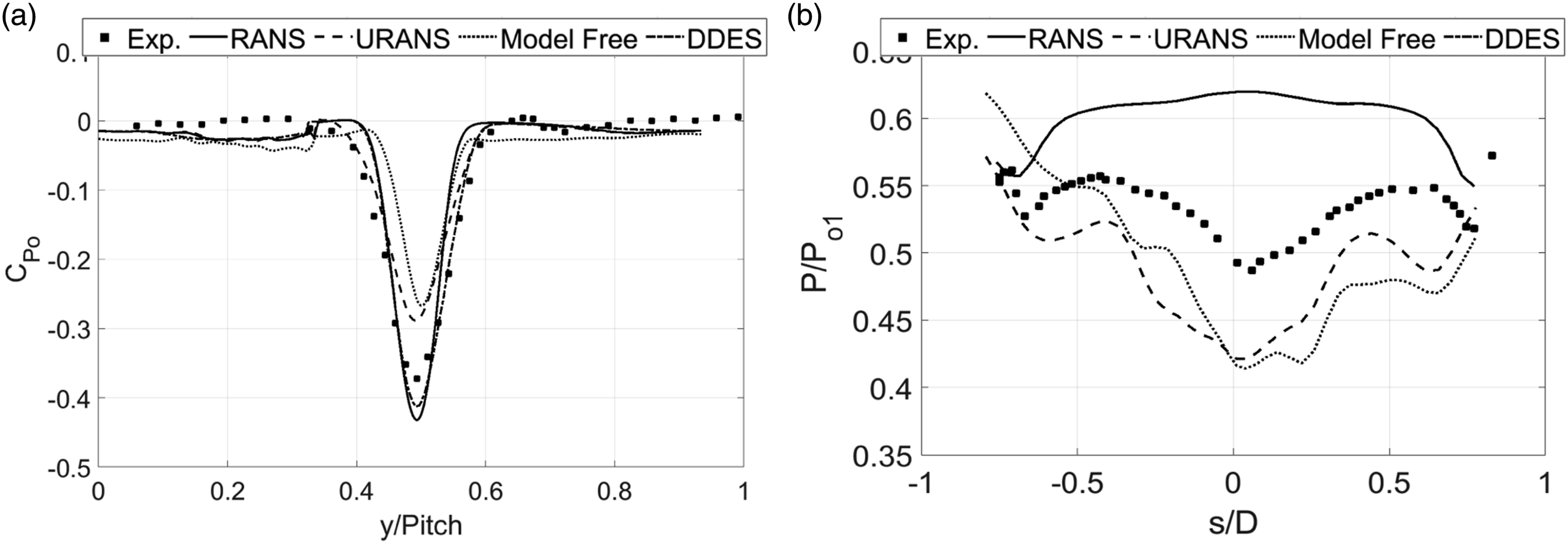

As described by Sieverding the pressure distribution along the trailing edge is characterized by three pressure minima: two caused by the Prandtl-Meyer expansion around the suction and pressure sides prior to flow separation and a third at the trailing edge center caused by the enrolment of the separating shear layers into a vortex core.¹⁹ In this case, none of the modeling approaches seem to be able to replicate the complex flow phenomena occurring at the trailing edge exactly. RANS modeling shows the largest discrepancy, predicting first a sharp rise in base pressure following the separation of the suction and pressure side shear layers followed up by a large pressure plateau towards the trailing edge centerline. The URANS approach is the only method to successfully predict the location of the three pressure minima, although the magnitude is significantly lower than the experimental data. The model free approach was unable to predict the pressure side expansion location and subsequent pressure minima, but the location of the centerline and suction side minima are correctly captured. It should be noted that the predicted base pressure distributions shown above are similar to previous numerical results using URANS and RANS methods.¹³

Mean flow

Figures 9 and 10 show the time averaged, mixed-out total pressure loss coefficient as well as the mass flow averaged total flow turning at the evaluation plane for each of the loading and modeling strategies considered. All methods, with the exception of the URANS approach, predict a gradual rise in mixed-out total pressure loss coefficient from critical to limit loading. The sharp rise in loss prediction for the URANS model at the critical loading condition is explored in detail later; however, in summary this is due to the inability of the URANS method to accurately predict the transition from trailing edge dominated vortex formation to shock dominated vortex formation.

Figure 9.

Time averaged, mixed-out total pressure loss coefficient at each loading condition.

Figure 10.

Time averaged, mass flow averaged total flow turning at each loading condition.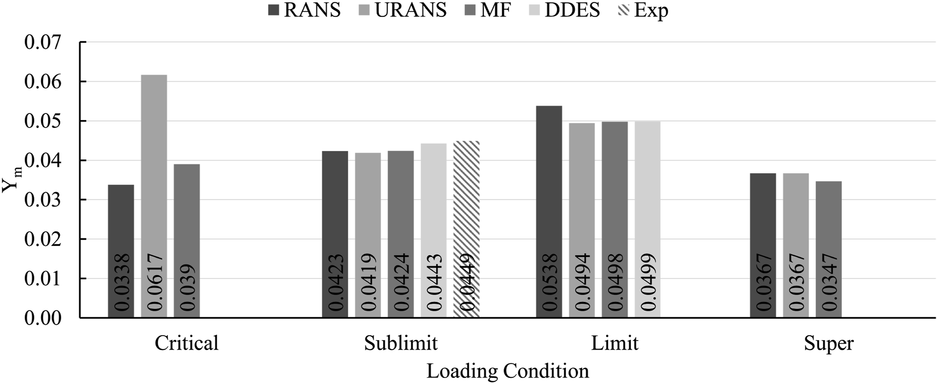

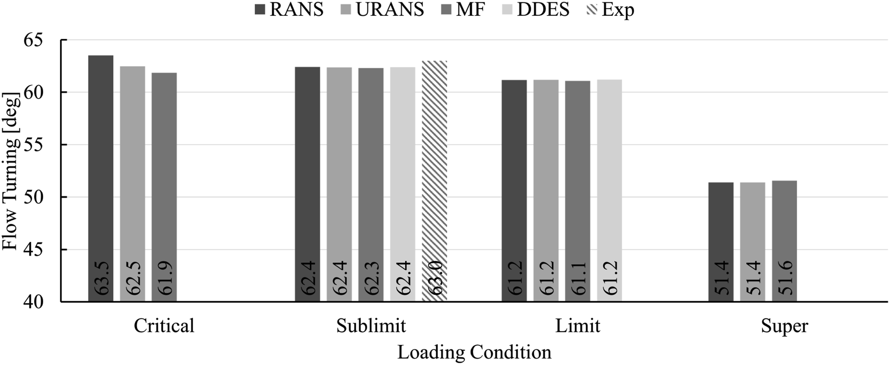
For all methods considered there is a sharp decline in loss coefficient from limit to super critical loading. This was unanticipated, as the total pressure loss was expected to increase with pressure ratio.^1,3,5 However, as the passage becomes fully choked, the oblique Trailing Edge Pressure Side Shock (TEPSS) caused by the rapid expansion around the trailing edge, completely clears the adjacent airfoil base pressure region resulting in reduced total pressure loss as well as flow turning. The interactions of the shock system with the blade boundary layer and wake structures becomes small and thus the predicted total pressure loss is reduced. Although a decrease in total pressure loss is desirable, there is a significant detriment in the ability of the airfoil to produce the desired work output, as this is directly related to the total flow turning. Furthermore, the large change in outlet flow angle can drastically decrease the efficiency of downstream blade rows through a change in incidence angle. A quick interpolation of results from Owen,⁶ shows that for a change of incidence by less than 2°, such as the change from critical to limit loading, total pressure loss is expected to rise by roughly 1%. However, as the incidence angle is significantly changed $(> 9 °)$ , such as is the case for supercritical loading, the estimated loss increase is roughly 25%. Clearly this is not desirable, highlighting the importance for aero designers to understand the limit and supercritical loading conditions.

Shown in Figure 11, are the predicted blade loading distributions for each modeling strategy at each loading condition. The available experimental data of Sooriyakumaran has been included for completeness. As a reminder experimental test results are only available for the sublimit loading condition.

Figure 11.

Surface isentropic mach number distribution at each loading condition.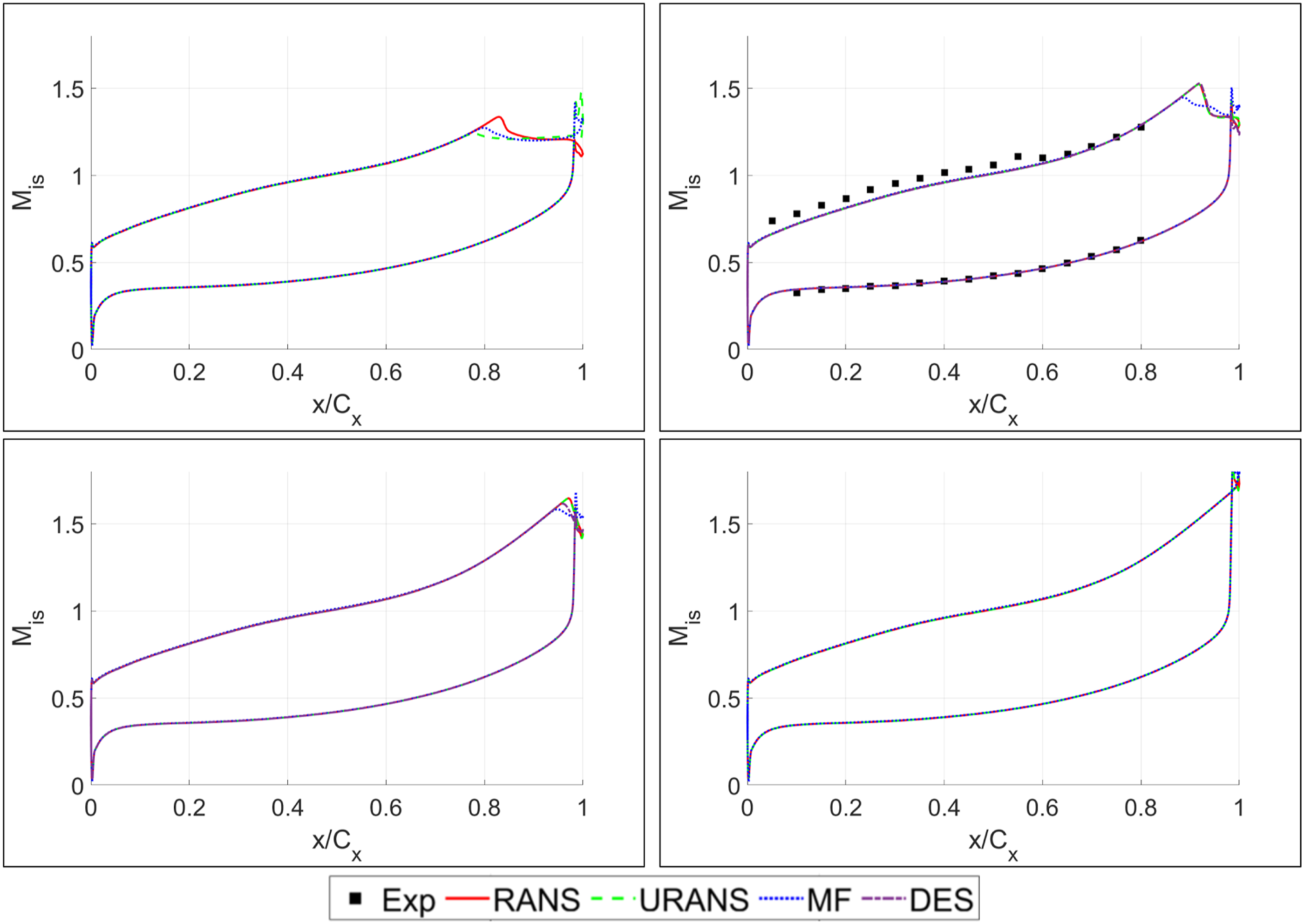

Blade loading distributions along the airfoil pressure surface as well as the suction surface prior to the location of shock interaction ( $\sim 0.8 C_{a x}$ for critical loading and $\sim 0.9 C_{a x}$ for sublimit) are predicted to be identical across loading conditions and modeling approaches. This is a result of flow choking cause by the trailing edge pressure surface shock (TEPSS). The effects of unsteady shock propagation and trailing edge vortex shedding are found to have a minimal effect on the flow field and subsequent blade loading. Downstream of the pressure side shock, highlighted in Figure 12, there are clear differences in the ability of each modeling approach to predict the shock propagation and subsequent shock/boundary layer interaction.

Figure 12.

Trailing edge surface isentropic mach number distribution at each loading condition.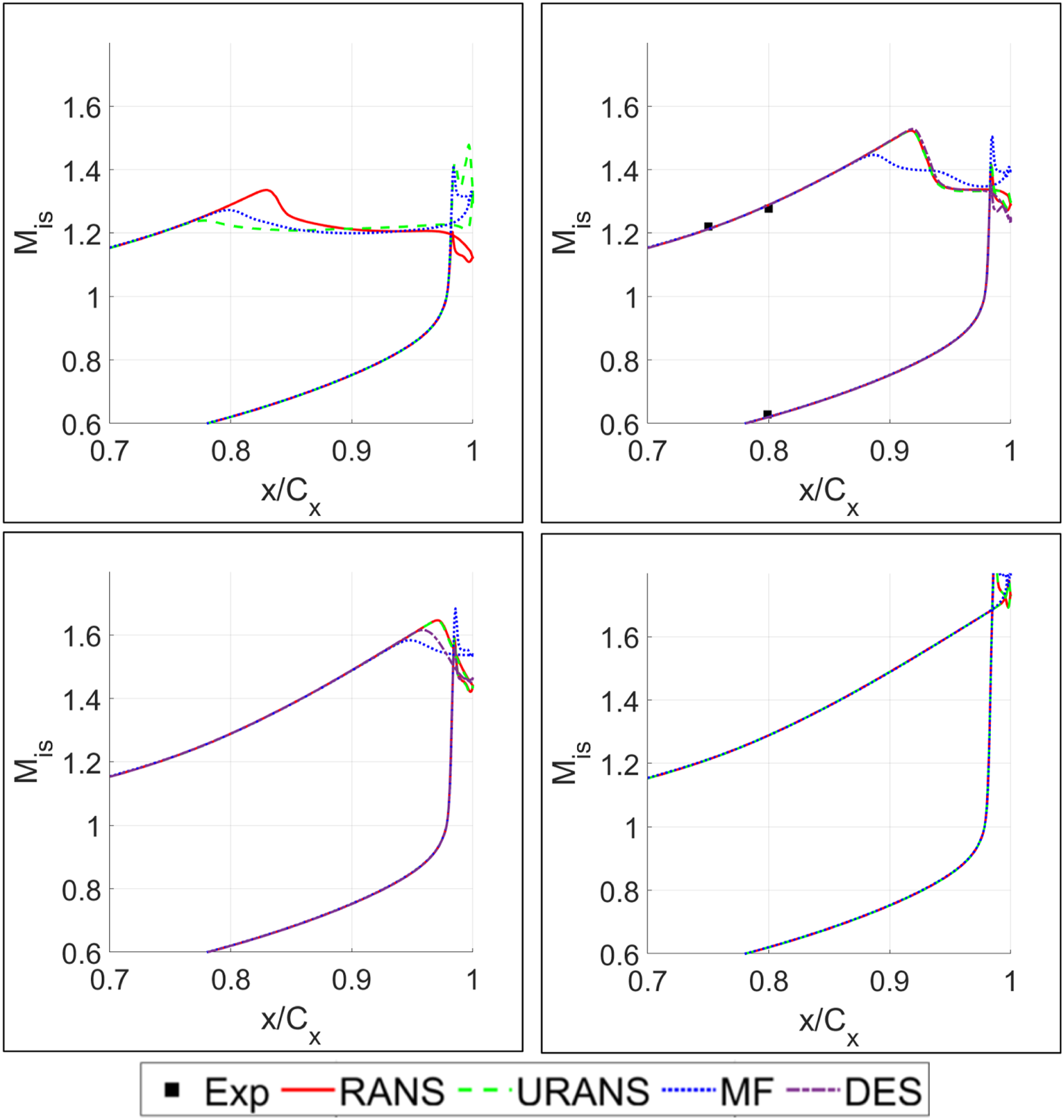

Unsteady propagation of the TEPSS caused by the interaction of the shock system with the trailing edge vortex shedding process causes the surface isentropic Mach number distribution to change. As the pressure surface shear layer is shed and rolled into a vortex core the shock system is weakened, resulting in an oscillatory shock effect. This system is then propagated downstream towards the adjacent airfoil causing a subsequent shock-boundary layer interaction which, in a time averaged sense, results in a smoothing of the shock impact.

This is most significant at lower pressure ratios where the predicted base pressure region is smaller, such as the critical loading condition. As illustrated through numerical Schlieren flow visualizations in a later section, the pressure and suction side shear layers do not achieve sufficient momentum to create a well-established base pressure region. This causes the trailing edge pressure side shock to form nearer the airfoil trailing edge resulting in significant influence from the vortex formation process. As the pressure ratio is increased, the base pressure region becomes established and causes vortex formation to occur downstream of the trailing edge shock system. All modeling approaches, with the exception of the model free strategy show minimal oscillation of the shock location as the base pressure region becomes established. Therefore, RANS/URANS and DDES all predict similar loading distributions for the sublimit loading conditions and above. As will be shown later, the model free approach predicts a much smaller base pressure region than the others, as is apparent in the base pressure distribution as well as flow visualizations. At supercritical loading all models predict near identical surface pressure distributions as the flow upstream of the TEPSS is fully choked and temporally stationary.

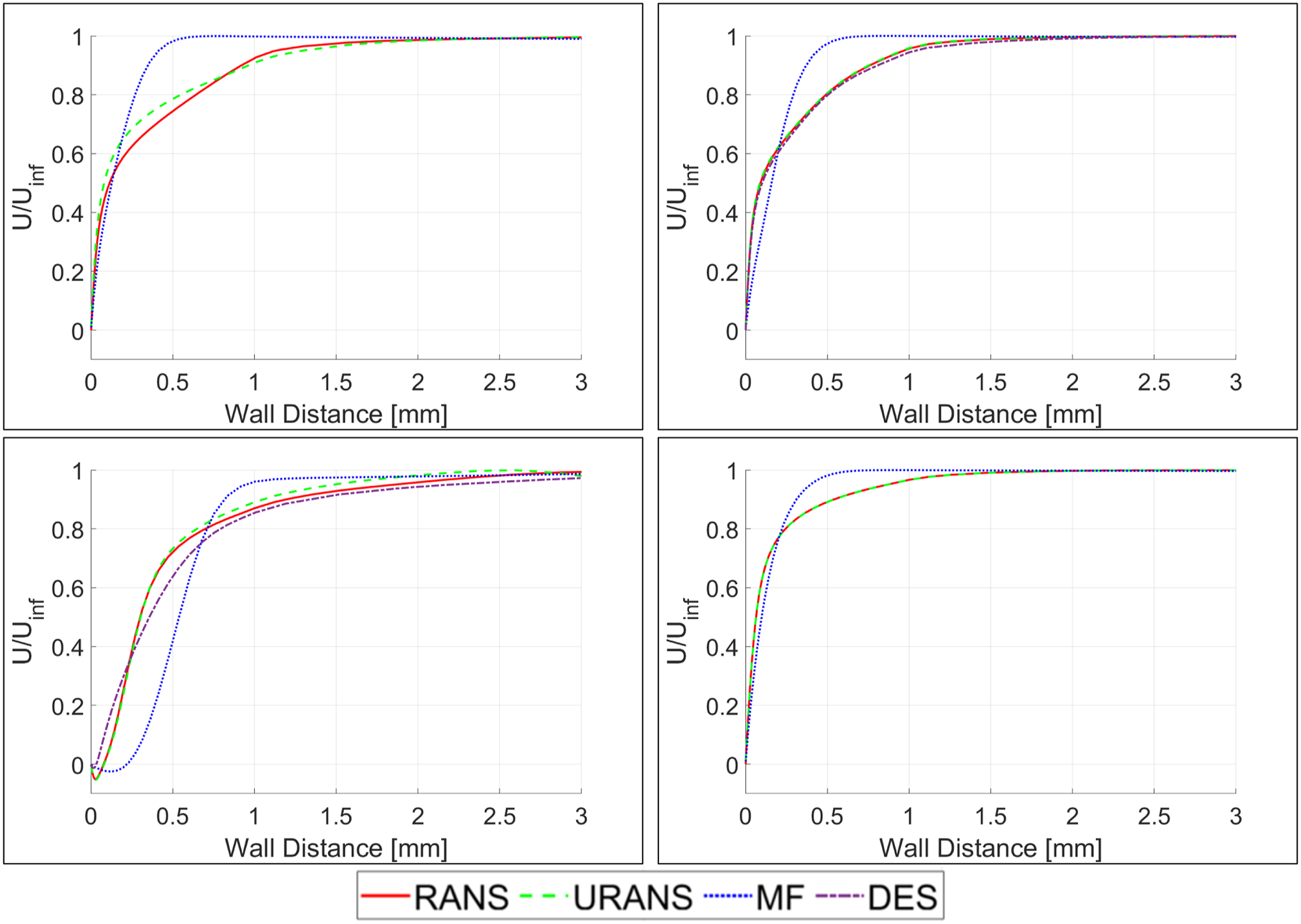
To further investigate the causes of the differences in vortex formation and subsequent downstream total pressure distributions, plots of the wall normal velocity on both the pressure and suction sides at 98% chord are presented in Figures 13 and 14. Due to the strong acceleration along the pressure surface, the boundary layer near the trailing edge of the pressure side is predicted to be laminar and near identical across loading conditions. The flow in this region is fully choked; therefore, any increase in pressure ratio only changes the flow downstream of the trailing edge pressure surface shock. The total boundary layer thickness, estimated as 99% of the freestream velocity, was predicted to be roughly 0.92 mm for the RANS, URANS and DDES simulations and 0.31 mm for the model free approach.

Figure 13.

Pressure side trailing edge boundary layer profiles.

Figure 14.

Suction side trailing edge boundary layer profiles.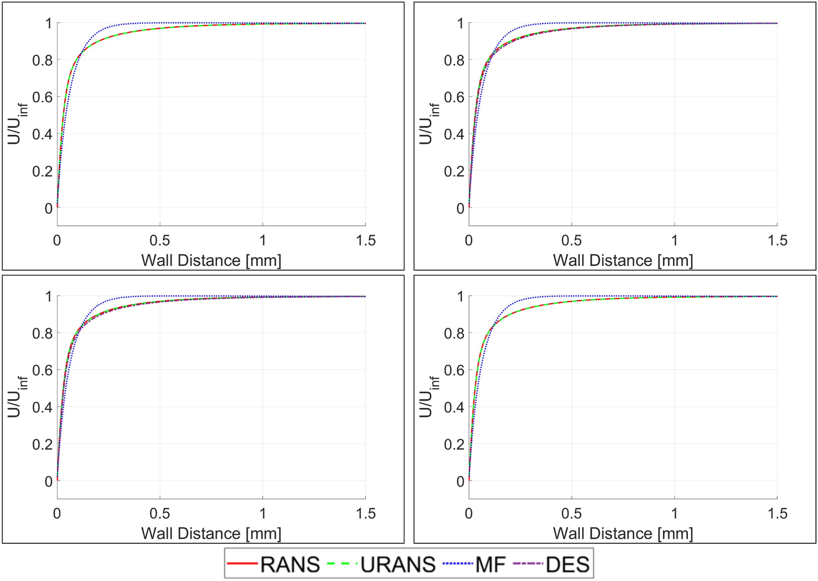

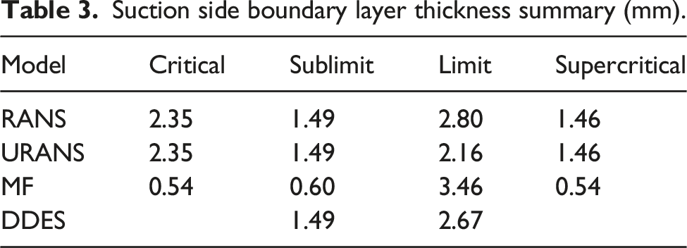
Unlike the pressure side, the suction side of the airfoil surface shows a strong dependence on load condition and modeling strategy, specifically for the limit loading condition. A summary of the predicted boundary layer thickness for each condition and strategy is shown in Table 3. At the lowest pressure ratio, the flow is clearly attached and turbulent with the exception of the model free strategy which alludes to a transitionary state. Similar to the pressure side RANS, URANS and DDES approaches all show similar boundary layer thickness and distribution for the sublimit loading condition with a total thickness of roughly 1.5 mm.

Table 3.

Suction side boundary layer thickness summary (mm).

Model	Critical	Sublimit	Limit	Supercritical
RANS	2.35	1.49	2.80	1.46
URANS	2.35	1.49	2.16	1.46
MF	0.54	0.60	3.46	0.54
DDES		1.49	2.67

As the pressure ratio is increased to limit loading the boundary layer profile shows a period of separation. This is a product of the influence of the trailing edge pressure side shock interacting with the suction side shear layer that forms one side of the base pressure region. The shock/base pressure interaction causes acoustic waves to propagate upstream creating a brief period of instability in the boundary layer. Although each modeling strategy shows separation, the magnitude is significantly different between strategies with the model free approach showing the largest region of flow recirculation. The approximate size and location of the period of separation requires a deeper look at the full flow picture and is investigated further with flow visualizations later in this report.

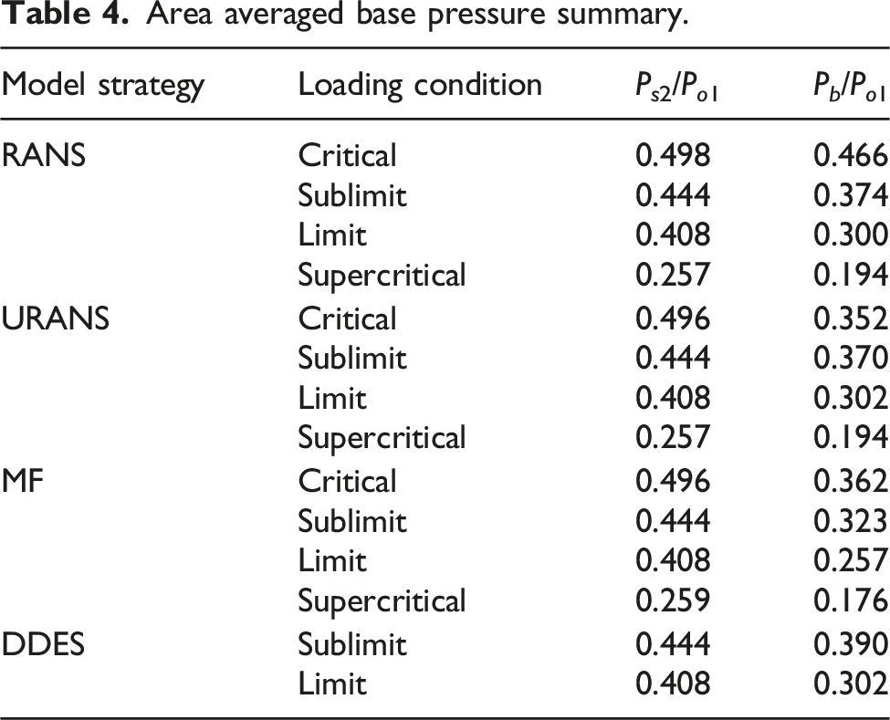
Figure 15 shows the predicted base pressure distribution for each modeling strategy and loading condition. For critical loading, the flow at the trailing edge is characterized by attached vortices formed by the alternating shedding of the pressure and suction side shear layers. The trailing edge pressure surface shock gains sufficient expansion to create an established base pressure region, resulting in a period of nearly constant pressure towards the trailing edge centerline. Local pressure minima are seen at the locations of the shear layer separation points and are a result of the Prandtl-Meyer expansion around the trailing edge. All modeling approaches predict the general trend of the pressure distribution similarly, although the unsteady formulations show a significantly lower base pressure than the steady RANS simulation for the critical loading condition. As the pressure ratio is increased towards limit loading the magnitude of the base pressure is lowered and is consistent for all modeling approaches. A summary of the normalized time and surface averaged base pressure is listed in Table 4 and presented alongside the well-known base pressure correlation created by Sieverding²⁰ in Figure 16.

Figure 15.

Base pressure distributions.

Table 4.

Area averaged base pressure summary.

Model strategy	Loading condition	P_s2/P_o1	P_b/P_o1
RANS	Critical	0.498	0.466
	Sublimit	0.444	0.374
	Limit	0.408	0.300
	Supercritical	0.257	0.194
URANS	Critical	0.496	0.352
	Sublimit	0.444	0.370
	Limit	0.408	0.302
	Supercritical	0.257	0.194
MF	Critical	0.496	0.362
	Sublimit	0.444	0.323
	Limit	0.408	0.257
	Supercritical	0.259	0.176
DDES	Sublimit	0.444	0.390
DDES	Limit	0.408	0.302

Figure 16.

Comparison with the base pressure correlation proposed by Sieverding.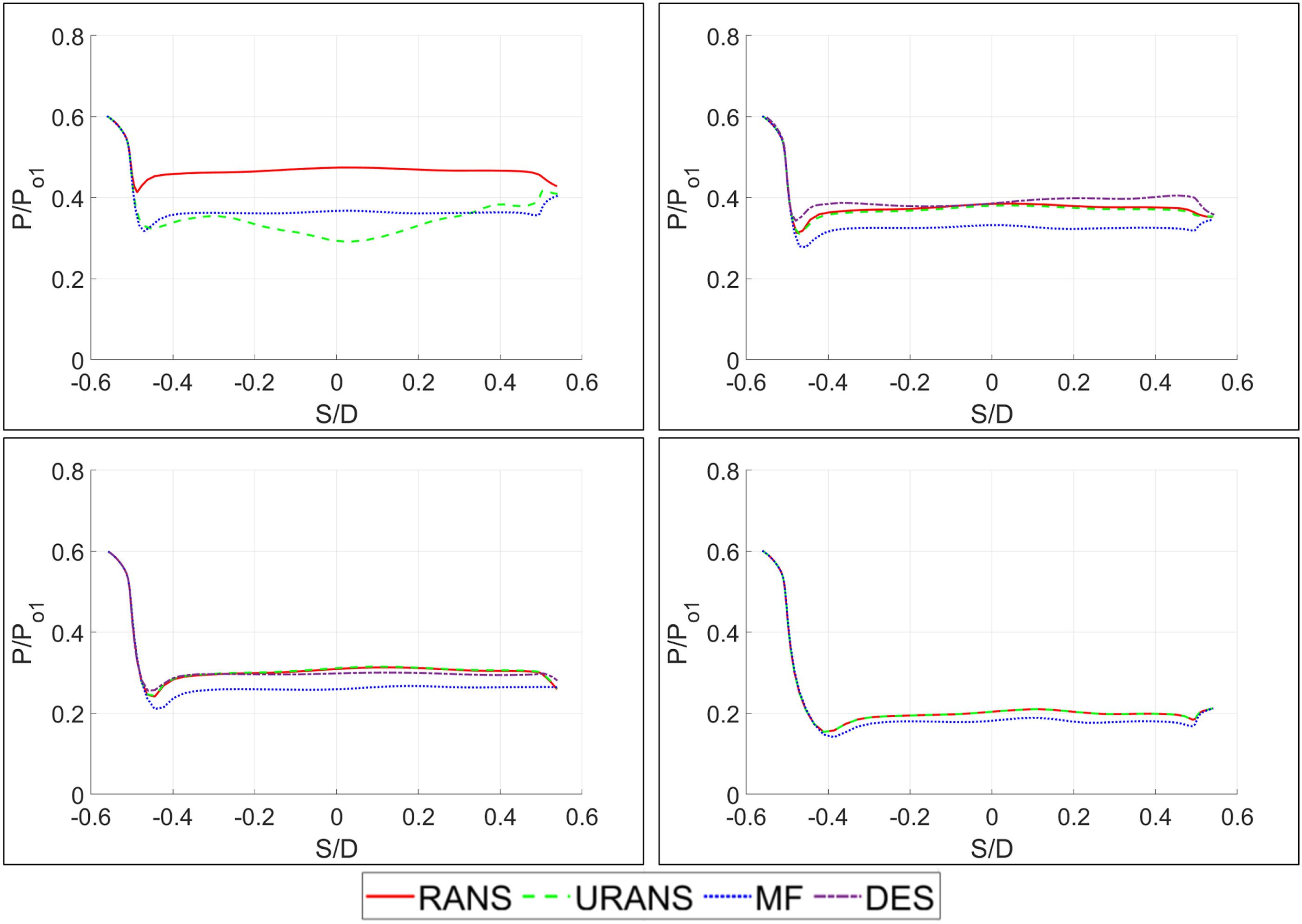

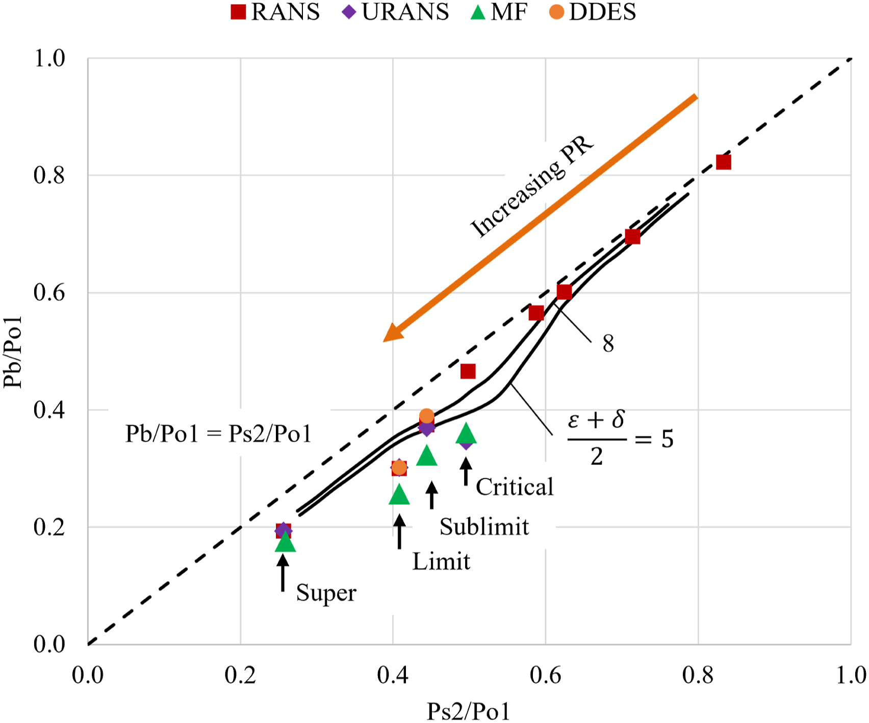
Results are distinguished as follows: RANS simulations as red squares, URANS simulations as purple diamonds, model free simulations as green triangles and DDES as orange circles. The solid lines show the correlation by Sieverding for the geometric properties nearest the investigated airfoil and the dashed line signifies equal base and downstream static pressures to help with analysis.

As the total pressure ratio is increased the predicted base pressure decreases for all modeling approaches. During critical loading each unsteady model predicts a significantly lower base pressure than steady RANS. As the pressure ratio is increased to sublimit and limit loadings the base pressure is predicted similarly for each of the wall modeled simulations, suggesting the flow is statistically stationary within the base pressure region. The model free approach predicts a much lower base pressure than the others for each of the loading conditions. This is a product of the size of the base pressure region, which is directly related to the magnitude and state of the pressure and suction side boundary layers near the trailing edge. As shown previously, the predicted model free boundary layers are much smaller than the other approaches. This causes the shear layer separation at the trailing edge to occur more rapidly, creating a stronger pressure side expansion. As the expansion becomes stronger the subsequent base pressure becomes lower.

Figure 17 shows the predicated time averaged total pressure loss distributions for each pressure ratio and modeling strategy. As observed in the mixed-out mass flow averaged total pressure loss coefficient, downstream losses increase with an increase in pressure ratio until supercritical loading. This is due to a combination of increased wake and freestream losses. During critical loading freestream losses are predicted to be small compared to wake losses as a result of how the vortices are being shed from the trailing edge. When the base pressure region is attached to the trailing edge, vortices shed quickly leading to increased mixing and wake losses.

Figure 17.

Downstream total pressure loss distributions.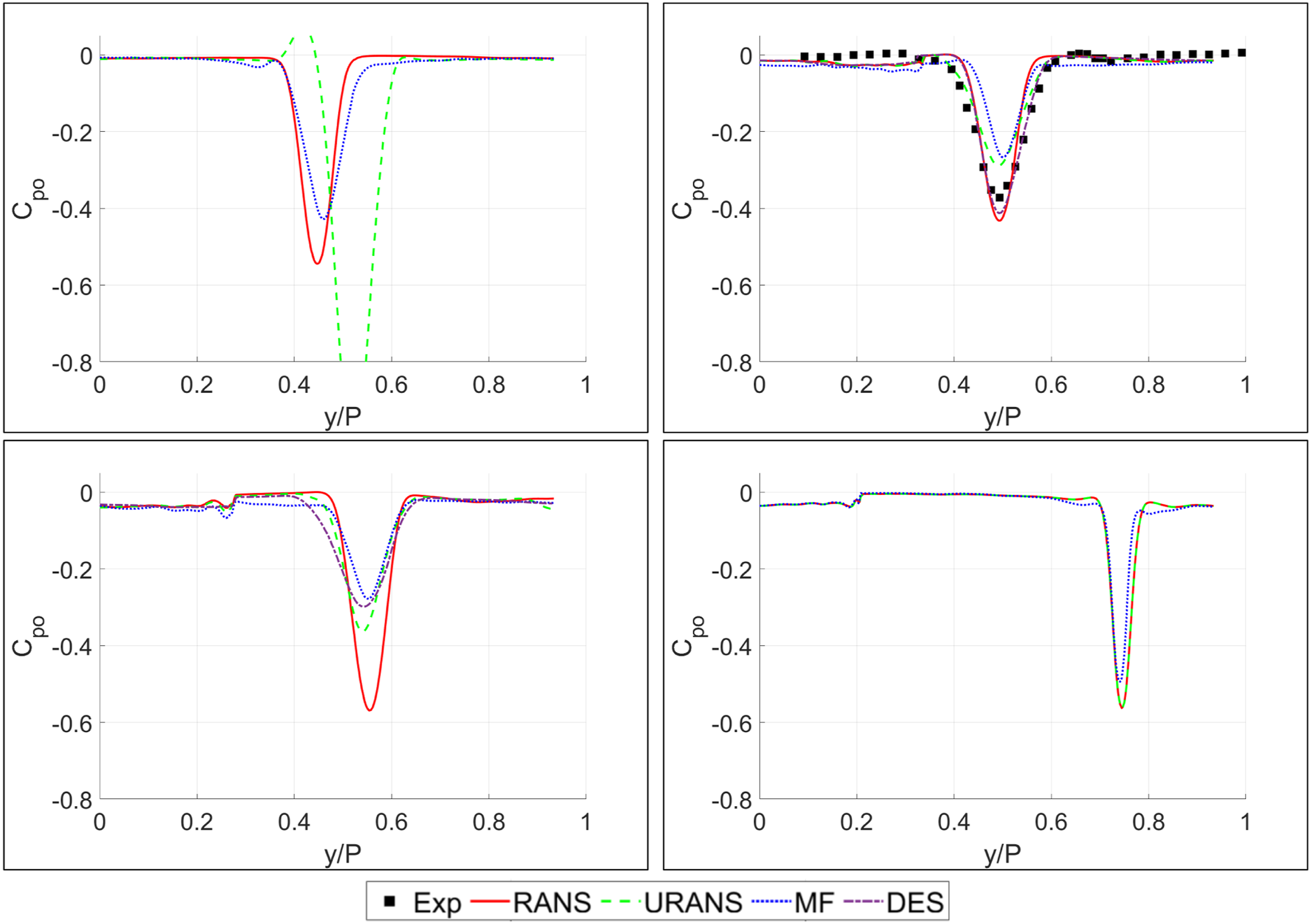

Increase of the pressure ratio to sublimit loading causes the flow expansion around the trailing edge to become stronger, leading to a larger and more established base pressure region that pushes vortex formation downstream as well as decreases the frequency of the vortex shedding. Although there is a reduction in wake losses, shock and freestream losses are increased. This is a product of the strong oblique trailing edge shock system, with the pressure side shock interacting with the suction surface boundary layer and the suction side shock propagating through the downstream wake. For limit loading the loss is further increased due to the complex flow near the trailing edge and base pressure region. As the TEPSS passes through the base pressure region acoustic waves propagate upstream along the suction surface followed by flow separation and increased wake width and depth. Also included is the impact of the suction side shock on the downstream wake profile. Predictions for super critical loading show that as the TEPSS departs the base pressure region, the influence of vortex formation becomes small and freestream losses are reduced for the majority of the domain.

Looking at the difference in modeling approaches, it is clear that the RANS simulations predict the smallest wake width and largest wake depth of the modelling strategies considered for all loading conditions. This is due to a lack of vortex/shock interactions. With the exception of critical loading, the URANS and model free approaches show a much smaller wake depth; however, due to vortex formation they predict an increase in wake width compared to RANS. The DDES approach, shown only for the sublimit and limit loading conditions, shows the widest wake prediction as well as best correlation with available experimental data.

During critical loading the URANS method predicted an unrealistic downstream loss profile. It should be noted the authors preformed a rigorous grid refinement study as well as manual time step adjustment to repair the downstream loss prediction. It was concluded that the URANS method failed to correctly predict the transition from near trailing edge vortex formation to shock trailing edge vortex formation at the edge of the base pressure region. Further analysis results are presented and discussed later in this paper.

Transient phenomena

Shown in Figure 18 are the normalized power spectral densities of the mass flow averaged total pressure loss coefficient at the evaluation plane for the critical, sublimit and limit loading conditions. Supercritical loading is not presented as the loss coefficient for each modeling approach remained temporally constant. This is believed to be a result of the choking of the flow caused by the trailing edge pressure surface shock. As can be seen there is a peak energy that clearly defines the vortex shedding frequency for each modeling approach.

Figure 18.

Power spectrum - mass-flow averaged total pressure loss coefficient. (a) URANS, (b) MF, (c) DDES.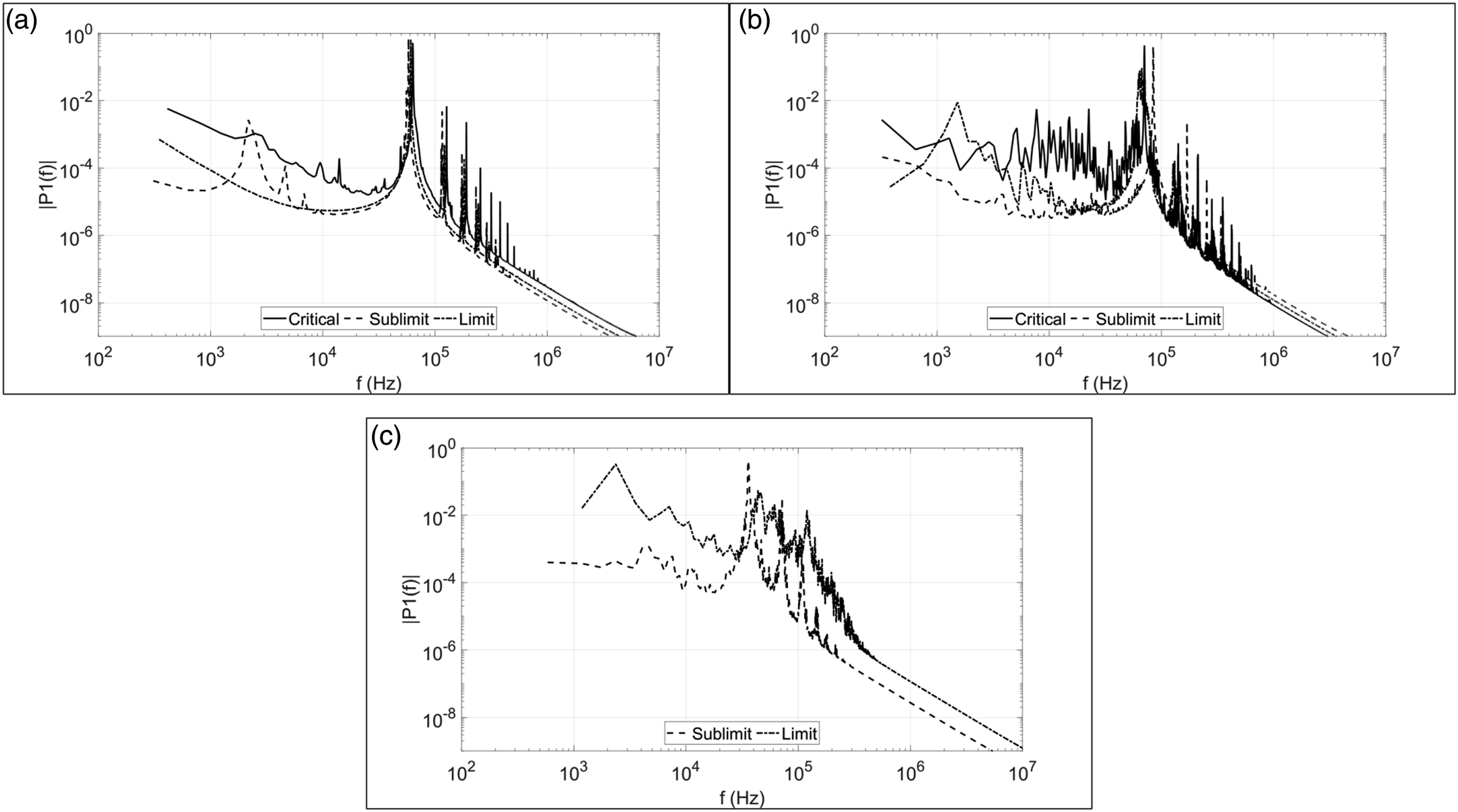

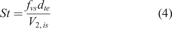
A summary of the peak vortex frequency, calculated Strouhal number and vortex shedding period is given in Table 5. The Strouhal number was computed using equation (4) with f_vs being the peak vortex shedding frequency, d_te the trailing edge diameter and V_2,is the mass flow averaged isentropic flow velocity at the evaluation plane.

S t = \frac{f_{v s} d_{t e}}{V_{2, i s}}

(4)

Table 5.

Power spectrum analysis summary.

Model strategy	Loading	Peak freq. (kHz)	Strouhal #	Vortex period (ms)
URANS	Critical	60.3	0.241	0.017
	Sublimit	58.1	0.217	0.017
	Limit	60.7	0.217	0.016
MF	Critical	70.2	0.279	0.014
	Sublimit	84.7	0.316	0.012
	Limit	63.0	0.226	0.016
DDES	Sublimit	35.9	0.134	0.028
DDES	Limit	46.2	0.165	0.022

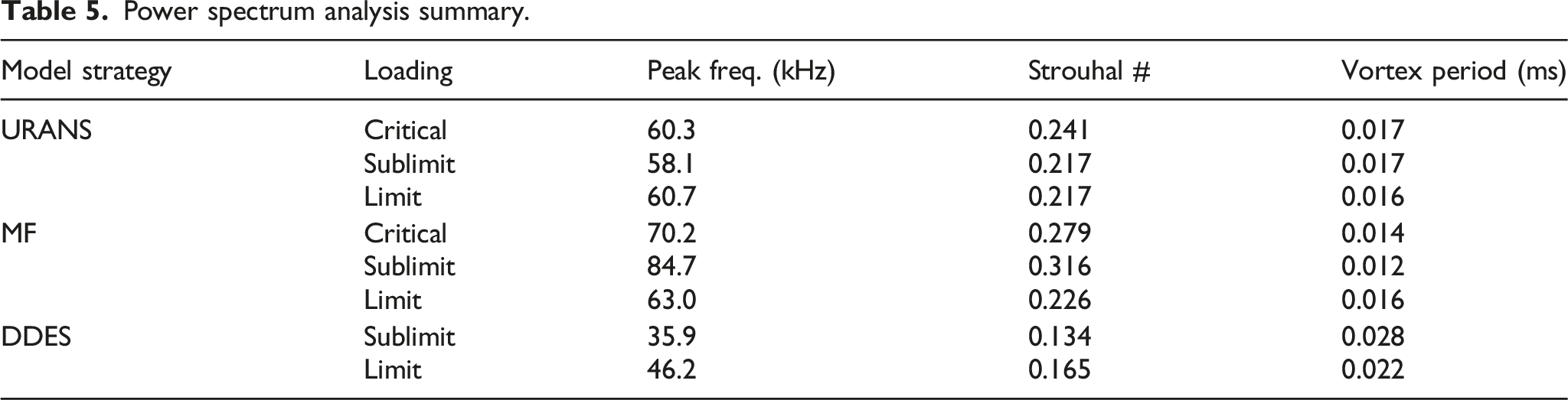
For each modeling strategy, the average adaptive time step required to produce a convective CFL number of less than one was smaller for higher total pressure ratios. Although there is a wide range of predicted Strouhal numbers between modeling strategies, they are all within the bounds of similar experimental and computational investigations.¹⁹ The model free simulation shows a much higher predicted vortex shedding frequency than the other unsteady methods for all loading conditions, with a peak difference occurring during sublimit loading. As discussed previously, this is a product of the state of the trailing edge boundary layer. The results of the URANS simulations predict lower Strouhal numbers than the model free approach; however, the DDES simulations predict Strouhal numbers to be much lower than either of the other methods. To help clarify the causes of the differences in vortex shedding frequency between modeling strategies flow visualizations of the normalized density gradient at various phase states are presented in the following section.

Critical loading

Figure 19 shows the URANS and model free visualizations of the instantaneous normalized density gradient for a full vortex shedding period. The left most images describe the point where the pressure side trailing edge vortex is initially shed and the right most image illustrates the point just prior to the next pressure side vortex period. Comparing modeling approaches, it is clear that the base pressure region, trailing edge shock structures and trailing edge boundary layers are predicted quite differently between methods.

Figure 19.

Normalized density gradient at the trailing edge - critical loading.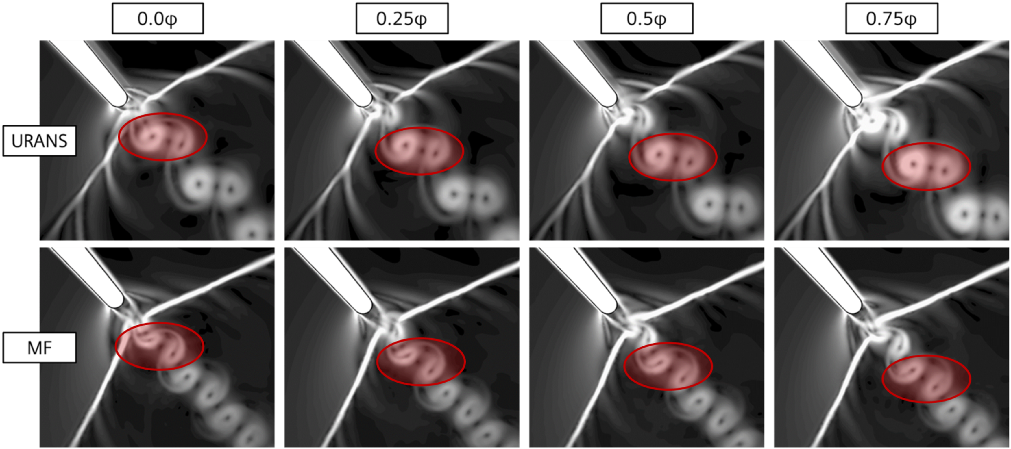

The URANS approach shows a much smaller base pressure region, with vortex formation occurring very near the trailing edge surface. In contrast the model free approach predicts a larger base pressure region with the shock clearly forming at the coalescence of the trailing edge pressure and suction side shear layers. This difference between model predictions results in an increase in vortex shedding period as shown in Table 5. In agreement with previous experimental work,^21,22 both modeling approaches show the pressure side shear layer to dominate the vortex shedding process. As described by Han and Cox this is due to the rapid expansion around the pressure side trailing edge, resulting in vortex pairs that have been highlighted in red.

Overall, predictions of the trailing edge shock system are quite different between modeling approaches with the URANS method predicting both the pressure and suction side shocks to be approximately normal to the airfoil outlet metal angle, while the model free approach suggests a more oblique shock structure. As described by Sieverding et al.,⁹ pressure waves initiate from the point of boundary layer separation on both the pressure and suction surfaces. These waves impinge on the suction side boundary layer resulting in the smearing of the blade loading distribution seen in Figures 11 and 12. The location and angle of the shock formation is directly related to the boundary layer state at the trailing edge which is clearly different between modeling strategies and has been documented previously through wall normal velocity profiles.

Sublimit loading

Figure 20 shows instantaneous predictions of the normalized density gradient for each modeling approach at the sublimit loading pressure ratio. As expected, each of the modeling strategies predicts an oblique trailing edge shock system that forms a well-established base pressure region. The flow expands rapidly around the trailing edge leading to a strong separated shear layer that coalesces into two distinct oblique shocks. The flow upstream of the shock is choked and therefore temporally stationary. The model free approach shows the only variation, although minute, of the flow prior to the suction surface shock. Referring back to the surface isentropic Mach number distributions presented in Figures 8 and 9 an explanation for the smearing of the model free shock impingement can be explained by highlighting the suction surface boundary layer. The flow separates slightly during the shock boundary layer interaction, resulting in slight fluctuations of the suction surface pressure distribution. In a time-averaged sense these pressure fluctuations merge into a smearing of the shock impingement.

Figure 20.

Normalized density gradient at the trailing edge - sublimit loading.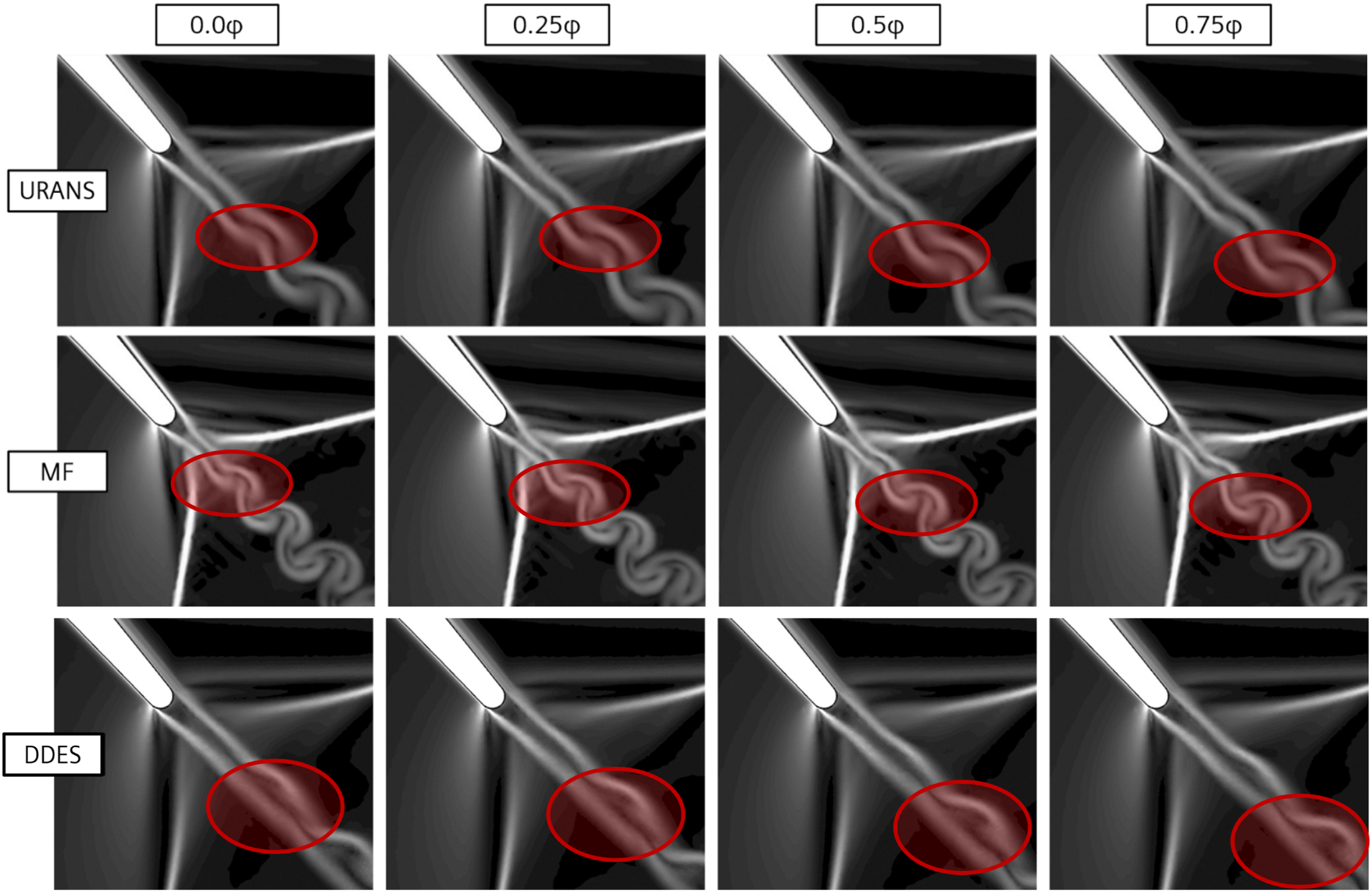

Similar to critical loading, the predicted von Karman vortex street for the model free approach is tighter and more frequent than the other unsteady methods. This is a result of the state of the trailing edge boundary layer and pressure side expansion. The model free approach shows a much smaller boundary layer than the other methods; that then causes the size of the base pressure region to shrink. This in turn results in tighter vortex pairs as well as closer trailing edge shocks. Both the URANS and DDES simulations predict the size of the base pressure region to be much larger than the model free approach. However, as can be seen the DDES predicts vortex formation to occur much farther downstream. This shows a direct relation to lower Strouhal numbers as shown in Table 5. As the base pressure region is predicted to be larger the Strouhal number or subsequent vortex shedding frequency is decreased.

Limit loading

Lastly the instantaneous predictions of the limit loading condition are presented in Figure 21. Clearly, the flow is intrinsically complex, showing a combination of shock/boundary layer interaction, Prandtl-Meyer expansion, vortex formation as well as flow separation. The rapid expansion around the trailing edge pressure side results in the formation of the base pressure region which then leads to the formation of the oblique trailing edge shock system. Vortices are then shed from the end of the base pressure region, still dominated by the pressure side flow expansion. The oblique pressure side shock, formed at the end of the base pressure region achieves sufficient flow turning to clear the suction surface of the adjacent airfoil and move into the base pressure region. This shock then interacts with the suction side shear layer, creating acoustic disturbances within the suction side boundary layer leading to flow separation upstream of the trailing edge.

Although each modeling approach clearly shows each of the previously described flow structures, the magnitude and location of each are different. The model free simulation predicts a much larger separation period along the suction surface than the other approaches as well as the smallest base pressure region. This combination, similar to what was discussed at sublimit loading, results in the highest predicted vortex frequency of the modeling strategies. Both the URANS and DDES approaches show similar base pressure sizes; however, the vortex formation downstream is drastically different between the methods. The vortices of the URANS simulation are much thinner and smaller than the DDES approach, resulting in the drastic reduction in the predicted Strouhal number for the DDES.

Figure 21.

Normalized density gradient at the trailing edge - limit loading.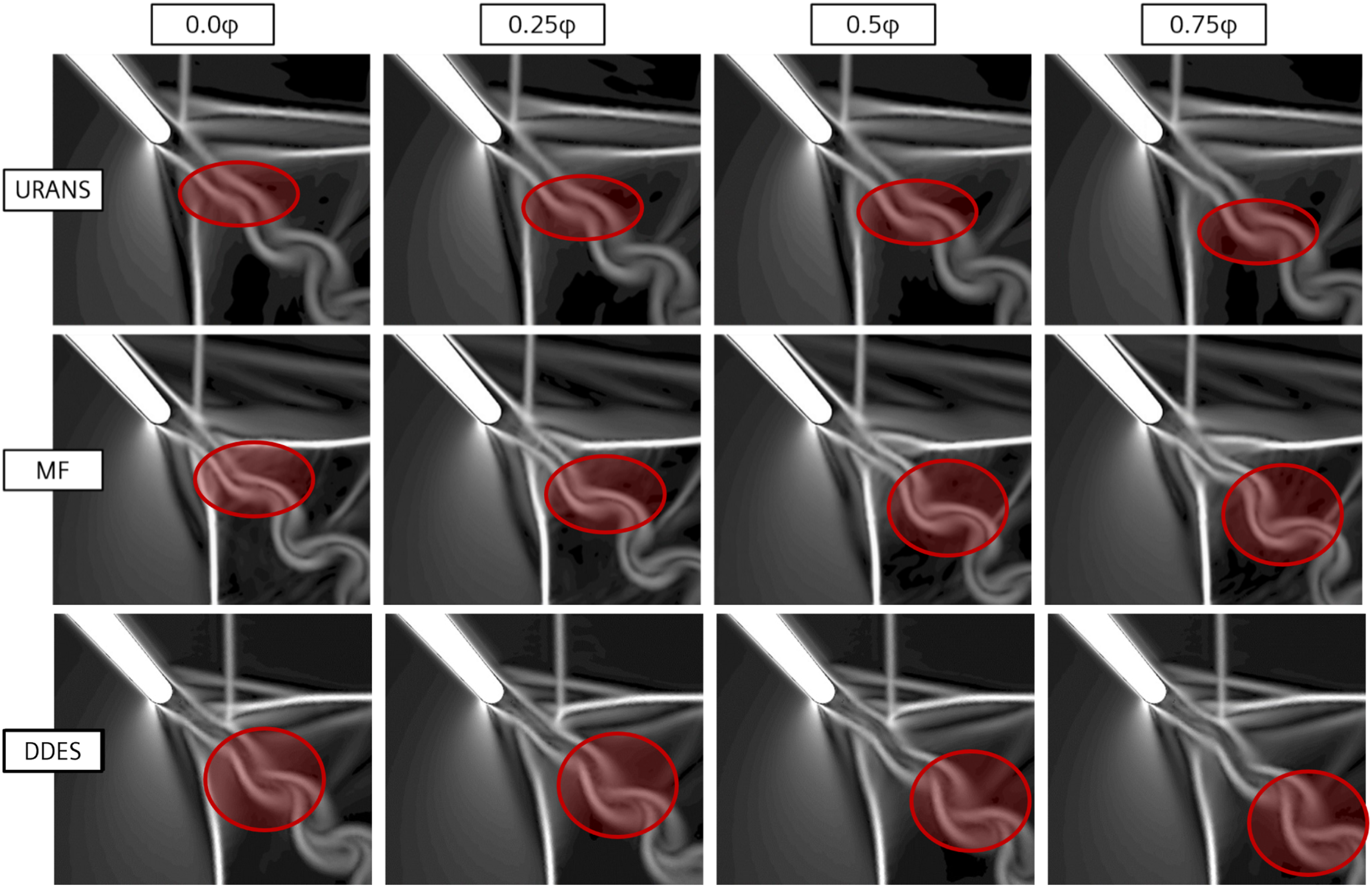

Conclusion

Similar to previous work,^3,23 as limit loading is reached the flow within the airfoil passage becomes fully choked and any further increase in pressure ratio fails to change the channel output. The influence of modeling strategies on the predicted mass-flow averaged total pressure loss coefficient, mass-flow averaged flow angles, and on the limit loading pressure ratio were found to be insignificant with the exception of the URANS model during critical loading. It was found that the URANS modeling approach failed to predict the transition from near trailing edge dominated vortex formation to aft base pressure vortex formation resulting in a drastic rise in predicted total pressure loss.

Surface isentropic Mach distributions were predicted similarly for all modeling strategies, with the exception of the trailing edge base pressure region and points of shock impingement along the suction surface. A smearing of the blade loading was predicted as a result of the relative position of the Trailing Edge Pressure Side Shock (TEPSS) and the point of vortex formation. When the TEPSS was predicted aft of the trailing edge vortex street, the oscillatory nature of the pressure side shear layer resulted in a fluctuating shock behavior that then propagated to the adjacent airfoil surface. As the pressure ratio was increased and the pressure side shear layer gained sufficient momentum to create a well-defined base pressure region, the oblique trailing edge shock was formed upstream of vortex formation resulting in a relatively stationary shock system.

A detailed review of the boundary layer states at the trailing edge reveals that all of the modeling approaches predicted laminar boundary layer profiles along the pressure surface trailing edge and turbulent profiles along the suction surface. In summary, the model free simulation approach predicted much smaller boundary layer thicknesses, unless separation occurred as did for the limit loading condition. Each modeling strategy predicted separation, although with varying degrees of size and magnitude, during limit loading along the suction side trailing edge caused by acoustic wave propagation of the interaction of the suction side shear layer and the TEPSS.

The predicted base pressure distributions were also reviewed, showing the base pressure to decrease with increasing pressure ratio. The unsteady simulation approaches consistently predicted lower average surface pressures than the steady state RANS simulations. As the pressure ratio was increased the RANS, URANS and DDES simulations all showed near identical predictions of the airfoil base pressure, suggesting the flow to be relatively stationary within the region. The model free approach showed a similar distribution; however overall magnitude of the base pressure deficit was increased for all loading conditions.

Temporal documentation of the mass flow averaged total pressure loss coefficient downstream of the airfoil allowed for the dominant vortex shedding frequency to be identified and subsequent Strouhal number to be calculated. It was found that the DDES approach predicted the lowest vortex frequency for both the sublimit and limit loading conditions. The model free approach predicted a much smaller base pressure region, resulting in a much higher vortex shedding frequency than the other methods. A formal documentation and review were made outlining the required simulation time step to achieve accurate temporal resolution as well as approximate vortex shedding period.

Qualitative images of the numerical Schlieren (normalized density gradient) contours were presented and reviewed showing large differences in the prediction of vortex shape, size and subsequent shock influence. This study suggests that for the prediction of general aerodynamic capabilities of turbine airfoils, such as blade loading distribution and downstream loss coefficients, RANS and URANS are sufficient while maintaining simulation efficiency for sublimit to limit loading conditions. Both MF and DDES approaches provide an additional level of predictive capability through the ability of Strouhal number determination as well as vortex structure characterization; however, without experimental documentation no concrete justification can be made at this time, further outlining the importance of an experimental investigation.

Footnotes

Author’s note

Permission for Use: The content of this paper is copyrighted by Siemens Energy, Inc. and is licensed to IMechE for publication and distribution only. Any inquiries regarding permission to use the content of this paper, in whole or in part, for any purpose must be addressed to Siemens Energy, Inc. directly.

Acknowledgements

The work described in this paper formed part of a PhD project at the University of North Carolina at Charlotte. The author wishes to thank the teaching and guidance of both Siemens Energy, Inc. and UNCC. A special thanks goes to Carlton University in providing the experimental results used for model validation.

Declaration of conflicting interests

The author(s) declared no potential conflicts of interest with respect to the research, authorship, and/or publication of this article.

Funding

The author(s) received no financial support for the research, authorship, and/or publication of this article.

ORCID iDs

Spencer Owen

Mesbah Uddin

Appendix

References

Hauser

Plohr

Sonder

. Study of flow conditions and deflection angle at exit of two-dimensional cascade of turbine rotor blades at critical and supercritical pressure ratios. NACA-RM E9K25, 1950.

Hauser

Plohr

. Two-dimensional cascade investigation of the maximum exit tangential velocity component and other flow conditions at the exit of several turbine blade designs at supercritical pressure ratios. NACA-RM E51F12, 1951.

Fruchtman

. The limit load of transonic turbine blading. ASME Paper No 74-GT-80, 1974.

Glassman

. Estimating turbine limit load. NASA CR-191105, 1993.

Chen

. Axial-flow turbine rotor discharge-flow overexpansion and limit-loading condition. Part 2; method of analysis and performance evaluation of computer code axod2. NASA/TM-2018-219911, 2018.

Owen

Taremi

Uddin

. Effect of inflow conditions on transonic turbine airfoil limit loading. Proc Inst Mech Eng A J Power Energy 2022; 236(5): 794–807.

Owen

. Numerical investigations on factors influencing limit loading for transonic turbine airfoils. PhD thesis. Charlotte, NC: The University of North Carolina at Charlotte, 2021.

Sooriyakumaran

. Experimental study of profile losses in three transonic turbine cascades. Master’s thesis. Ottawa, ON: Carelton University, 2014.

Sieverding

Richard

Desse

. Turbine blade trailing edge flow characteristics at high subsonic outlet mach number. J Turbomach 2003; 125(2): 298–309.

10.

Corriveau

Sjolander

. Influence of loading distribution on the performance of transonic high pressure turbine blades. J Turbomach 2004; 126(2): 288–296.

11.

Owen

Taremi

Uddin

. Turbulence modeling effects of transonic, high pressure airfoils near design incidence. AIAA Aviation 2019 Forum. ■■■: ■■■, 2019, p. 2965.

12.

Taremi

. Endwall flows in transonic turbine cascades. PhD thesis. Ottawa, ON: Carleton University, 2013.

13.

Léonard

Gicquel

Gourdain

, et al. Steady/unsteady reynolds-averaged navier–stokes and large eddy simulations of a turbine blade at high subsonic outlet mach number. J Turbomach 2015; 137(4): 041001.

14.

Lin

Yuan

. Local entropy generation in compressible flow through a high pressure turbine with delayed detached eddy simulation. Entropy 2017; 19(1): 29.

15.

Yang

Griffin

. Grid-point and time-step requirements for direct numerical simulation and large-eddy simulation. Phys Fluids 2021; 33(1): 015108.

16.

Agarwal

Konakalla

Selvan

. On meshing guidelines for large eddy simulations of gas turbine combustors. In: Proceedings of the ASME turbo expo 2014: turbine technical conference and exposition. Volume 4B: combustion, fuels and emissions, Düsseldorf, Germany, 16–20 June, 2014, p. V04BT04A011. American Society of Mechanical Engineers.

17.

Liou

. A sequel to ausm, part ii: Ausm+-up for all speeds. J Comput Phys 2006; 214(1): 137–170.

18.

Siemens . Star-ccm+ user manual. https://docs.sw.siemens.com/en-US/product/226870983/doc/PL20190509110447511.starccm/custom/ (2021, last accessed 19 February 2021).

19.

Sieverding

Manna

. A review on turbine trailing edge flow. Int J Turbomach Propuls Power 2020; 5(2): 10.

20.

Sieverding

Stanislas

Snoek

. The base pressure problem in transonic turbine cascades. ASME. J Eng Power 1980; 102(3): 711–718. American Society of Mechanical Engineers.

21.

Han

Cox

. A visual study of turbine blade pressure-side boundary layers. J Eng Power 1983; 105(1): 47–52.

22.

Currie

Carscallen

. Simulation of trailing edge vortex shedding in a transonic turbine cascade. J Turbomach 1998; 120(1): 10–19.

23.

Chen

. Axial-flow turbine rotor discharge-flow overexpansion and limit-loading condition, part 1: computational fluid dynamics (cfd) investigation. NASA/TM-2017-219506, 2017.

A characterization of unsteady effects for transonic turbine airfoil limit loading

Abstract

Keywords

Introduction

Numerical methods

Airfoil description

Boundary and initial conditions

Modeling strategies

Convergence criterion and time step

Grid description and convergence

2D/3D RANS and URANS comparison

Results and discussion

Validation

Mean flow

Transient phenomena

Critical loading

Sublimit loading

Limit loading

Conclusion

Footnotes

Author’s note

Acknowledgements

Declaration of conflicting interests

Funding

ORCID iDs

Appendix

References