Sage Journals: Discover world-class research

Abstract

In order to improve the efficiency of high-speed train aerodynamic noise analysis and provide a feasible method for aerodynamic noise prediction, the aerodynamic noise and its influencing factors are analyzed from the perspective of the total energy (sound power) radiated to the far field per unit time by the aerodynamic fundamental noise sources (monopole, dipole and quadrupole sources). A full-scale and a 1:8 scale-down computational fluid dynamics model of a high-speed train are established. The far-field sound pressure level at several receivers and velocities is calculated by using the transient large eddy simulation and the FW-H equation. The numerical simulation results are used to predict the aerodynamic noise under specified working conditions. The research work can achieve the prediction of aerodynamic noise at other velocities using noise data at known velocities on the same noise source case, as well as the prediction of aerodynamic noise of full-scale model using data of scale-down model, and is applicable to either bogies as local noise sources or the complete vehicle as a noise source. The maximum error between the prediction and simulation result is 0.33 dBA under various working conditions, which meets the engineering calculation requirements.

Keywords

High-speed train aerodynamic noise numerical simulation similarity criteria scale-down model

Introduction

During high-speed train operation, the aerodynamic noise generated by the train’s external aerodynamic action grows with the 4th-8th power of the vehicle speed, and its growth rate is much higher than that of the traction noise and the wheel-rail noise.¹ When the speed exceeds 300 km·h⁻¹, aerodynamic noise will become the main noise source of high-speed trains.² Excessive aerodynamic noise will reduce passenger comfort, affect the life and work quality of people along the line, especially in hospitals, schools, residential areas and other noise-sensitive areas, and even damage the hearing and nervous system of people inside and outside the car.^3–6 In China, aerodynamic noise pollution is considered to be one of the largest environmental pollution factors produced by high-speed railways to the society. According to the “14th Five-Year Plan of Action for Noise Pollution Prevention and Control”, the equipment selection of urban rail vehicles and the construction of rail lines and roadbed structures should comply with the requirements for the prevention and control of noise pollution in urban rail transport. In the international community, vibration noise has been listed as one of the seven major environmental hazards. Therefore, the research on prediction and control of aerodynamic noise of high-speed trains will directly affect the further speed up of high-speed trains, the sustainable development of high-speed rail transport, and the happiness index of people’s life.

In recent years, many scholars have conducted research on aerodynamic characteristics, generation mechanism of aerodynamic noise sources and noise distribution characteristics of high-speed trains.^7,8 Sunil et al.⁹ investigated the aerodynamic characteristics of locomotives using Computational Fluid Dynamics (CFD) numerical simulation method to study the locomotive head configuration, and used Multi-Objective Optimization Method (MOOM) to optimize the locomotive configuration with locomotive drag and aerodynamic lift as optimization parameters. The results showed that the adopted optimization technique effectively improves the optimization performance and the aerodynamic characteristics of the locomotive head. Mo et al.¹⁰ modeled hydrodynamic models for three-to six-vehicle trains and analyzed their aerodynamic noise, showing that the train length basically does not affect the far-field noise distribution pattern. Zhang et al.¹¹ modeled a five-vehicle maglev train, and found that the distribution of dipole and quadrupole sources was basically the same at different speeds, which were distributed in the radio terminal area of the vehicle body and the wake area. Wang et al.^12–14 used wind tunnel tests and numerical simulations for the bogie area to investigate the effect of dipole sources generated by the main noise source components in the flow field. In addition, he also derived the far-field sound pressure level relationship between two objects with similar aerodynamic acoustics by means of wind tunnel tests. Li et al.¹⁵ studied near-field quadrupole noise sources and far-field aerodynamic noise with the aid of a scale-down model of the head car of a high-speed train, and found that turbulence around the head car has multi-scale vortex characteristics separated from the geometry and that volumetric dipole sources are the main source of near-field quadrupole noise. Li et al.^7,16 compared and analyzed the aerodynamics, flow field characteristics, surface pressure and far-field noise of pantograph models of different scales. The results showed that the far-field aerodynamic noise of pantographs was less affected by the scale of the model, but as the scale decreased, the energy concentration range of the radiated noise changed from low to medium-high frequency. In addition, with the help of numerical simulation and wind tunnel test, Li also analyzed the superposition relationship between the noise radiated from the local aerodynamic noise source to the far field and the overall noise source of the far field of the high-speed train. The results showed that the step-by-step numerical prediction method of aerodynamic noise of high-speed train is practically meaningful. At present, most of the scientific research work is to explore the aerodynamic characteristics, the aerodynamic noise sources characteristics and noise radiation characteristics of high-speed trains. It is more conducive to the analysis and prediction of aerodynamic noise by analyzing and exploring the influence of noise source on far-field aerodynamic noise from the theoretical perspective.

A new method for predicting the aerodynamic noise of high-speed trains is proposed. Numerical simulations are carried out for scale-down and full-scale models, and the aerodynamic noise of different working conditions is predicted and analyzed based on similar criteria. The research work provides new ideas for aerodynamic noise prediction and reduction, and provides a feasible method to solve the problems of large number of meshes, long calculation time and low efficiency in numerical simulation.

Numerical simulation method for aerodynamic noise

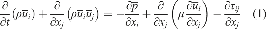
Computational Aerodynamic Acoustics (CAA) uses numerical computational methods to study the non-constant flow mechanism of noise generated by the interaction between fluid and solid boundaries in order to provide a systematic theoretical basis for noise prediction and improvement.¹⁷ For high-speed trains with complex shapes and many components, ANSYS Fluent software is used to solve the generation and propagation processes of aerodynamic noise separately using a hybrid solution method.

(a) Firstly, the steady-state calculation is carried out using the Standard $k - ε$ turbulence model to obtain the steady-state solution of the external flow field of the high-speed train. The steady state solution is used as an initial value for subsequent transient calculations.

(b) For the transient part (sound field calculation), the Lighthill stress tensor ( $T_{i j}$ ) on the vehicle surface is calculated by Large Eddy Simulation (LES) with the steady state solution of the flow field as the initial state in order to construct the Lighthill equation. The propagation characteristics of the sound field, such as sound pressure level (SPL), frequency and total SPL at the receivers are obtained by applying the FW-H acoustic comparison method.

The pulsation and mixing of turbulence is mainly caused by large-scale eddies, which dominate the fluid's motion situation, receive energy from the main flow, and transfer the energy to the small-scale eddies. The small-scale vortices dissipate the received energy. The basic idea of LES is to calculate the pulsation of large-scale eddies by transient N-S equations, however, it does not calculate the small-scale eddies directly, but simulates the airflow influence of small-scale eddies by establishing sublattice model. In other words, the effects caused by turbulent pulsations are described in terms of vortex viscosity on the basis of vortex viscosity. The basic control equation for LES is shown as

\frac{\partial}{\partial t} (ρ {\bar{u}}_{i}) + \frac{\partial}{\partial x_{j}} (ρ {\bar{u}}_{i} {\bar{u}}_{j}) = - \frac{\partial \bar{p}}{\partial x_{i}} + \frac{\partial}{\partial x_{j}} (μ \frac{\partial {\bar{u}}_{i}}{\partial x_{j}}) - \frac{\partial τ_{i j}}{\partial x_{j}}

(1)

\frac{\partial ρ}{\partial t} + \frac{\partial}{\partial x_{i}} (ρ {\bar{u}}_{i}) = 0

(2)

Where

(^{-})

are the filtered field variable;

τ_{i j}

is the subgrid scale stress.

The above equation can be calculated to obtain the Lighthill stress tensor ( $T_{i j}$ ), which is used to construct the Lighthill source term. Lighthill derived the Lighthill equation by transforming the fluid continuity equation and the momentum equation and using the pulsating pressure as an independent variable.⁸ The Lighthill equation is written as

\frac{\partial^{2} ρ^{'}}{\partial τ^{2}} - c_{0}^{2} \nabla^{2} ρ^{'} = \frac{\partial^{2} T_{i j}}{\partial x_{i} \partial x_{j}}

(3)

where

ρ^{'}

is the fluid density fluctuation;

τ

is time;

c_{0}

is the velocity of sound at infinity;

\nabla

is the Hamilton operator;

T_{i j}

is the Lighthill stress tensor;

x_{i}

and

x_{j}

are the coordinate components; the right-hand side of the equation is the Lighthill source term.

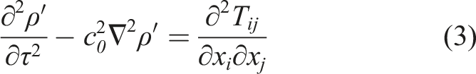
In the above equation, the left side of the equation is the acoustic equation. The right side of the equation consists entirely of the flow field parameters, which can be obtained by experiment or fluid calculation to decouple the noise problem.

Ffowcs Williams and Hawkings extended the Lighthill acoustic analogy theory to the problem of fluid flow sounding in the presence of arbitrary solid boundaries, resulting in the FW-H equation, which is defined as

\begin{array}{l} (\frac{1}{c_{0}^{2}} \frac{\partial^{2}}{\partial t^{2}} - \nabla^{2}) (H c_{0}^{2} ρ^{'}) \\ = \frac{\partial}{\partial t} {[ρ (u_{j} - v_{j}) + ρ_{0} v_{j}] \frac{\partial H}{\partial x_{j}}} \\ - \frac{\partial}{\partial x_{i}} {[ρ u_{i} (u_{j} - v_{j}) + P_{i j}] \frac{\partial H}{\partial x_{j}}} + \frac{\partial^{2} (H T_{i j})}{\partial x_{i} \partial x_{j}} \end{array}

(4)

where

t

is time;

H

is the Heaviside function;

u_{i}

is the component of fluid velocity in the

x_{i}

direction;

u_{j}

is the component of fluid velocity in the

x_{j}

direction;

v_{j}

is the component of surface velocity in the

x_{j}

direction;

P_{i j}

is the compressive stress tensor;

ρ

is the fluid density when disturbed;

ρ_{0}

is the fluid density when undisturbed.

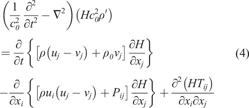
The first term on the right-hand side of the equation is the monopole source due to surface acceleration; the second term is the dipole source due to surface pulsation pressure; and the third term is the Lighthill source term (quadrupole source).

High-speed train aerodynamic noise prediction methods

This section investigates the relationship between the far-field radiation characteristics of both local and global noise sources of high-speed trains and the size of the noise source, the location of the receiver and the fluid velocity. Similar criteria for the prediction of aerodynamic noise from high-speed trains are analyzed.

Far-field aerodynamic noise under point noise sources

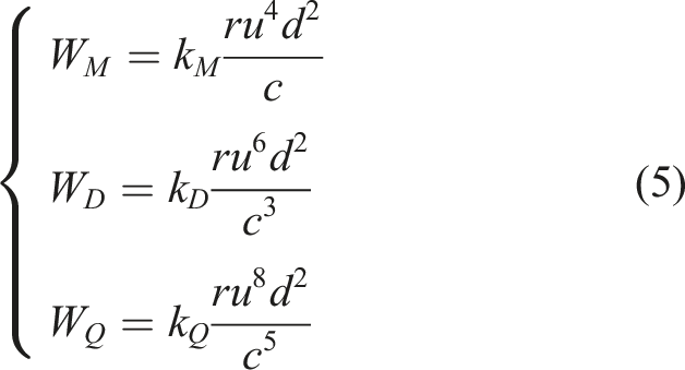
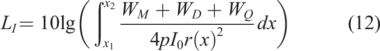
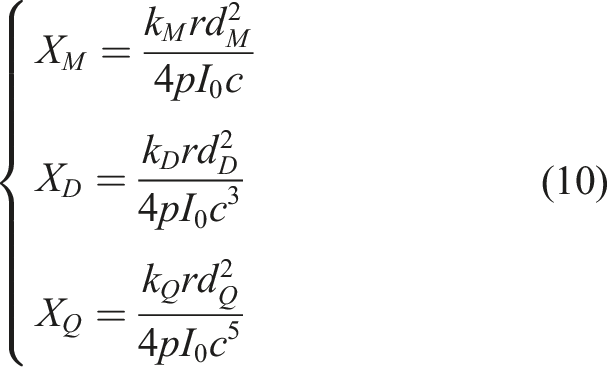
Aerodynamic noise sources can be divided into monopole, dipole and quadrupole sources. The radiated sound power is directly proportional to the 4th, 6th and 8th power of the airflow velocity respectively.¹⁸ The sound power of the three sources is defined as

{\begin{cases} W_{M} = k_{M} \frac{r u^{4} d^{2}}{c} \\ W_{D} = k_{D} \frac{r u^{6} d^{2}}{c^{3}} \\ W_{Q} = k_{Q} \frac{r u^{8} d^{2}}{c^{5}} \end{cases}

(5)

Where

W_{M}

W_{D}

, and

W_{Q}

are the sound power radiated by the three acoustic sources;

k_{M}

k_{D}

and

k_{Q}

are the scaling factors and are constants;

ρ

is the air density;

u

is the velocity of the acoustic source;

d

is the characteristic size of the acoustic source;

c

is the sound speed.

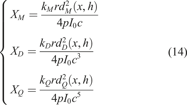
In fluid acoustics calculations, the geometry is often very complex. The size of the characteristic ( $d$ ) needs to be selected according to the influence of the different geometrical features on the flow pattern. When analyzing the far-field aerodynamic noise of high-speed train bogies, the size of the noise source is small in relation to the propagation distance and the noise source is not very directional, so the noise source can be reduced to a point noise source. Considering its influence on the flow pattern, the characteristic size of the bogie is defined as the bogie height to calculate the $R e$ number.

For the noise prediction work in this section, the volumes and distribution of the three basic noise sources in bogie area are different. When reducing all the noise sources in this region to a single point consisting of a monopole source, a dipole source and a quadrupole source, setting the characteristic size of the three basic sources to the height of the bogie cannot accurately represent the noise source volumes of this region and need to be expressed as $d_{M}$ , $d_{D}$ and $d_{Q}$ respectively.

The sound intensity produced by a point noise source in a free sound field is

L_{I} = 10 \lg \frac{I}{I_{0}}

(6)

I = \frac{p^{2}}{ρ c} = \frac{W}{4 π r^{2}}

(7)

Where

L_{I}

is sound intensity level;

I

is sound intensity at the receiver;

I_{0}

is reference sound intensity;

p

is the sound pressure at the receiver;

W

is the sound power;

r

is the distance between the receiver and the noise source.

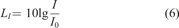
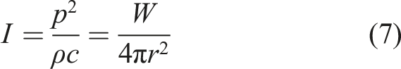
The sound intensity is in accordance with the principle of superposition. So the sound intensity generated by the point noise source can be considered as the sum of the sound intensity generated by the monopole source, dipole source and quadrupole source at the same point. According to equation (6) and (7), the sound intensity can be defined as

\begin{array}{l} L_{I} = 10 \lg \frac{I_{M} + I_{D} + I_{Q}}{I_{0}} \\ = 10 \lg \frac{W_{M} + W_{D} + W_{Q}}{4 π r^{2} I_{0}} \end{array}

(8)

Where

I_{M}

I_{D}

, and

I_{Q}

are the sound intensities of the three noise sources respectively.

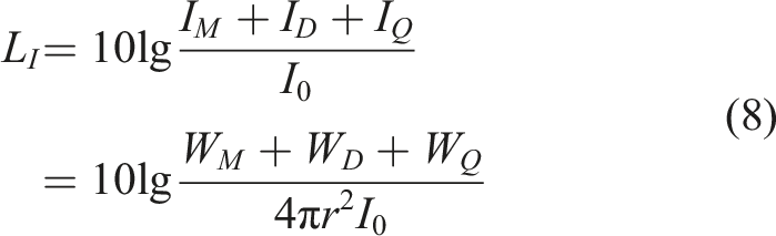
Sound intensity and sound pressure are different, but when air density and sound velocity are not considered, the sound intensity level and SPL are equal, expressed as $L_{I} = S P L$ . Substitute equation (5) into equation (8) to obtain the theoretical formula for SPL.

S P L = 10 \lg \frac{X_{M} u^{4} + X_{D} u^{6} + X_{Q} u^{8}}{r^{2}}

(9)

{\begin{cases} X_{M} = \frac{k_{M} r d_{M}^{2}}{4 p I_{0} c} \\ X_{D} = \frac{k_{D} r d_{D}^{2}}{4 p I_{0} c^{3}} \\ X_{Q} = \frac{k_{Q} r d_{Q}^{2}}{4 p I_{0} c^{5}} \end{cases}

(10)

Where

X_{M}

X_{D}

, and

X_{Q}

are undetermined coefficients.

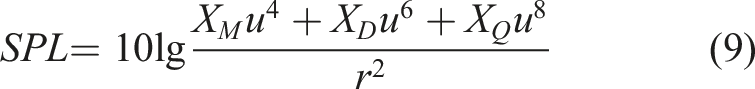
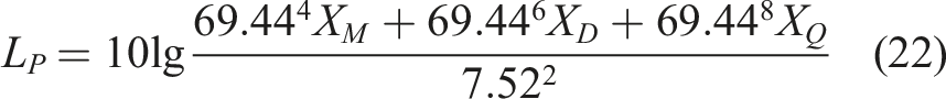
The above equation shows that SPL generated by a point noise source is dependent on the undetermined coefficients, the velocity of movement ( $u$ ) and the distance between the receiver and the noise source ( $r$ ). The undetermined coefficients are only related to the characteristic size of the source ( $d$ ), so if the noise source and the characteristic size remain the same, the undetermined coefficients remain the same.

Far-field aerodynamic noise under line noise sources

When the complete vehicle of the high-speed train is regarded as a noise source, it can be considered as a line noise source consisting of several point sources along the centerline of the vehicle. This source radiates noise in the form of an approximate columnar surface wave. The characteristic size of the vehicle body is determined by vehicle height ( $d$ ), which facilitates the calculation of $R e$ number.

The main noise source areas of the whole vehicle include the head vehicle, bogies, a pantograph and others, which have more noise sources than other areas. The volumes of the three basic noise sources are also different from one another. When the vehicle is considered as a line noise source consisting of several points, each consisting of a monopole source, a dipole source and a quadrupole source, the characteristic size of the three sources cannot be unified as the height of the vehicle, but are related to the location of the point in order to accurately express the volumes of noise sources in different areas of the vehicle.

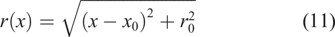
The longitudinal distance between a point on the line noise source and the front of the vehicle ( $x$ ) is considered as the independent variable, and $d$ is considered as the dependent variable. Considering that the size of the vehicle body will affect the characteristic dimensions, the vehicle height ( $h$ ) is listed as one of the influencing factors for $d$ . At this point, $d$ becomes $d (x, h)$ , and the $d (x, h)$ of the three aerodynamic fundamental noise sources at this point can be expressed as $d_{M} (x, h)$ , $d_{D} (x, h)$ , and $d_{Q} (x, h)$ respectively. In addition, $x$ also affects the distance between the point and receiver ( $r (x)$ ). The relationship between $d (x, h)$ , $r (x)$ and $x$ for any point on the centerline of the vehicle body is shown in Figure 1.

Figure 1.

Feature size and distance of point noise source.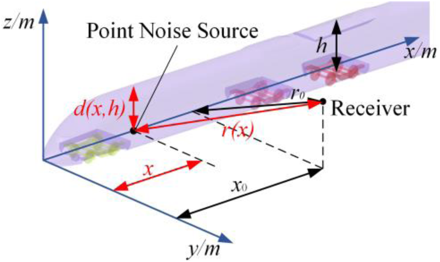

In the figure above, $x_{0}$ is the longitudinal distance between the receiver and the front of the vehicle. $r (x)$ is also related to the vertical distance from the receiver to the centerline of the vehicle ( $r_{0}$ ), as shown in the following equation.

r (x) = \sqrt{{(x - x_{0})}^{2} + r_{0}^{2}}

(11)

According to the sound intensity superposition principle, the sound intensity level at the receiver is superimposed by the sound intensity generated at several points along the centerline of the vehicle. Each point consists of three basic sound sources, as shown in the following equation.

L_{I} = 10 \lg (\int_{x_{1}}^{x_{2}} \frac{W_{M} + W_{D} + W_{Q}}{4 p I_{0} r {(x)}^{2}} d x)

(12)

Where

x_{1}

and

x_{2}

are the x-axis coordinates of the end points of the front and rear of the vehicle respectively; the integrated function is the ratio of the sound intensity generated by the three noise sources at a certain point on the centerline of the vehicle to the reference sound intensity.

Substituting equations (5) and (11) into the above equation, the far-field SPL of the line source can be expressed as

S P L = 10 \lg \int_{x_{1}}^{x_{2}} \frac{X_{M} u^{4} + X_{D} u^{6} + X_{Q} u^{8}}{{(x - x_{0})}^{2} + r_{0}^{2}} d x

(13)

{\begin{cases} X_{M} = \frac{k_{M} r d_{M}^{2} (x, h)}{4 p I_{0} c} \\ X_{D} = \frac{k_{D} r d_{D}^{2} (x, h)}{4 p I_{0} c^{3}} \\ X_{Q} = \frac{k_{Q} r d_{Q}^{2} (x, h)}{4 p I_{0} c^{5}} \end{cases}

(14)

Since it is difficult to obtain a specific function expression for

d (x, h)

to calculate the integral, the parameters containing

x

are integrated to obtain the following formula for calculating the far-field aerodynamic noise of a line noise source.

S P L = 10 \lg \frac{X_{M}^{'} u^{4} + X_{D}^{'} u^{6} + X_{Q}^{'} u^{8}}{r_{0}^{2}}

(15)

{\begin{cases} X_{M}^{'} = \frac{k_{M} ρ}{4 π I_{0} c} \int_{x_{1}}^{x_{2}} \frac{d_{M}^{2} (x, h) r_{0}^{2}}{{(x - x_{0})}^{2} + r_{0}^{2}} d x \\ X_{D}^{'} = \frac{k_{D} ρ}{4 π I_{0} c^{3}} \int_{x_{1}}^{x_{2}} \frac{d_{D}^{2} (x, h) r_{0}^{2}}{{(x - x_{0})}^{2} + r_{0}^{2}} d x \\ X_{Q}^{'} = \frac{k_{Q} ρ}{4 π I_{0} c^{5}} \int_{x_{1}}^{x_{2}} \frac{d_{Q}^{2} (x, h) r_{0}^{2}}{{(x - x_{0})}^{2} + r_{0}^{2}} d x \end{cases}

(16)

Where

X_{M}^{'}

X_{D}^{'}

and

X_{Q}^{'}

are undetermined coefficients.

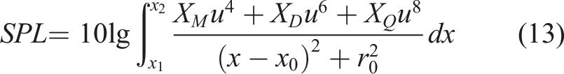
The analysis of the above equation shows that the undetermined coefficients is related to the vehicle size ( $h$ , $x_{1}$ , $x_{2}$ ) and the location of the receiver ( $x_{0}$ , $r_{0}$ ). Keeping the vehicle dimensions and receivers constant, the undetermined coefficients can be obtained using the data at the three speeds.

Similarity criteria of aerodynamic noise in high-speed trains

According to the literature, aerodynamic acoustic prediction studies need to comply with the geometric similarity criterion, $M a$ number, $R e$ number, $S t$ number and $E u$ number similarity criteria.^19,20 In the aerodynamic noise prediction work of this paper, in order to ensure the accuracy of the prediction results, it is also necessary to ensure that the above parameters in the similarity model satisfy the similarity condition.

The research work consists of predicting the far-field SPL at a receiver of the same model, and predicting SPL at the corresponding scale receivers of the full-scale model using scale-down model data. For the former, all similar parameters of the same model are unchanged and the similarity criteria are satisfied, while for the latter, a similarity analysis is required. The scale-down model corresponds proportionally to the full-scale model in terms of vehicle body dimensions and receivers coordinates, so geometric similarity conditions can be satisfied; Numerous studies on aerodynamic noise similarity relations have shown that the $S t$ number similarity criterion is not used in the pre-design stage of similar models, but in the post-processing stage, which is to calculate the prototype noise frequency by the model noise frequency.²⁰ In contrast, this study is aimed at predicting and analyzing SPL in the far field, without considering the frequency factor, so there is no need to analyze the similarity of $S t$ number; for free turbulence without gravity, $E u$ number is not considered. In summary, the similarity of $M a$ number and $R e$ number need further analysis.

(1) $M a$ number similarity analysis

The formula for calculating $M a$ number is

M a = \frac{u}{c}

(17)

The velocity of sound (

c

) does not vary in the research work. The similarity model and the numerical simulation model have equal fluid velocities and

M a

number similarity criterion is satisfied.

(2) $R e$ number similarity analysis

The formula for calculating $R e$ number is

R e = \frac{ρ u d}{μ}

(18)

The fluid velocity is equal in the scale-down model and the full-scale model. Air density is taken as

ρ = 1.205 k g / m^{3}

and viscosity coefficient as

μ = 1.82 \times 10^{- 5} N / m^{2} s

. The characteristic sizes (

d

) are taken as the height of vehicles (

d = 0.484 m

in the scale-down model and

d^{'} = 3.872 m

in the full-scale model). Calculations yielded

R e = 2.3 \times 10^{6}

in the scale-down model at 250 km·h⁻¹, and

R e^{'} = 1.8 \times 10^{7}

in the full-scale model at 250 km·h⁻¹.

R e \neq R e^{'}

, which clearly does not satisfy the

R e

number similarity criterion. However, studies have shown that when

R e

number is greater than the critical

R e

number (related study has shown that the critical

R e

number is

3.6 \times 10^{5}

R e

number enters the self-mode region and the aerodynamic characteristics no longer vary with

R e

number.²¹ At this point,

R e

number does not have a large effect on the non-constant aerodynamic acoustic similarity relationship.²² Therefore, the prediction work satisfies the

R e

number similarity criterion.

Comparison and analysis of numerical simulation and prediction results

High-speed train aerodynamic noise calculation model

Geometric model establishment

A full-scale and a 1:8 scale-down geometric model of CRH3 3-vehicle multiple unit are established, as shown in Figure 2. The model includes the head vehicle, intermediate vehicle, rear vehicle and six simplified bogies, retaining the deflector and pantograph deflector. The full-scale model is 72 m long and the scale-down model is 9 m long.

Figure 2.

Simplified geometric model of high-speed train. (a) The complete vehicle, (b) the bogie section.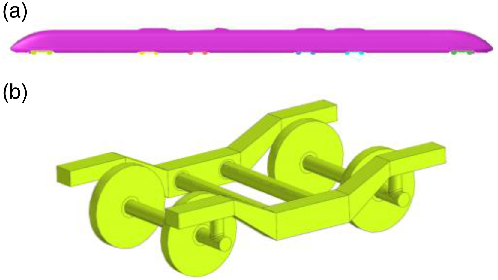

Calculation domain and boundary condition settings

The aerodynamic calculation domain of the scale-down model of high-speed train is shown in Figure 3. The calculation domain is 44 m long. The inlet of the flow field is 10 m from the front of the vehicle (greater than one time the length of the vehicle) and the outlet is 25 m from the rear of the vehicle (greater than 2 times the length of the vehicle). The width of the flow field is 8 m (more than 10 times the width of the vehicle) and the height is 5 m (more than 10 times the height of the vehicle). The length, width and height of the full-scale model calculation domain are 402 m (150 m from the front of the vehicle at the inlet and 180 m from the rear of the vehicle at the outlet), 80 m and 50 m respectively.

Figure 3.

Scale-down model calculation domain and boundary setting.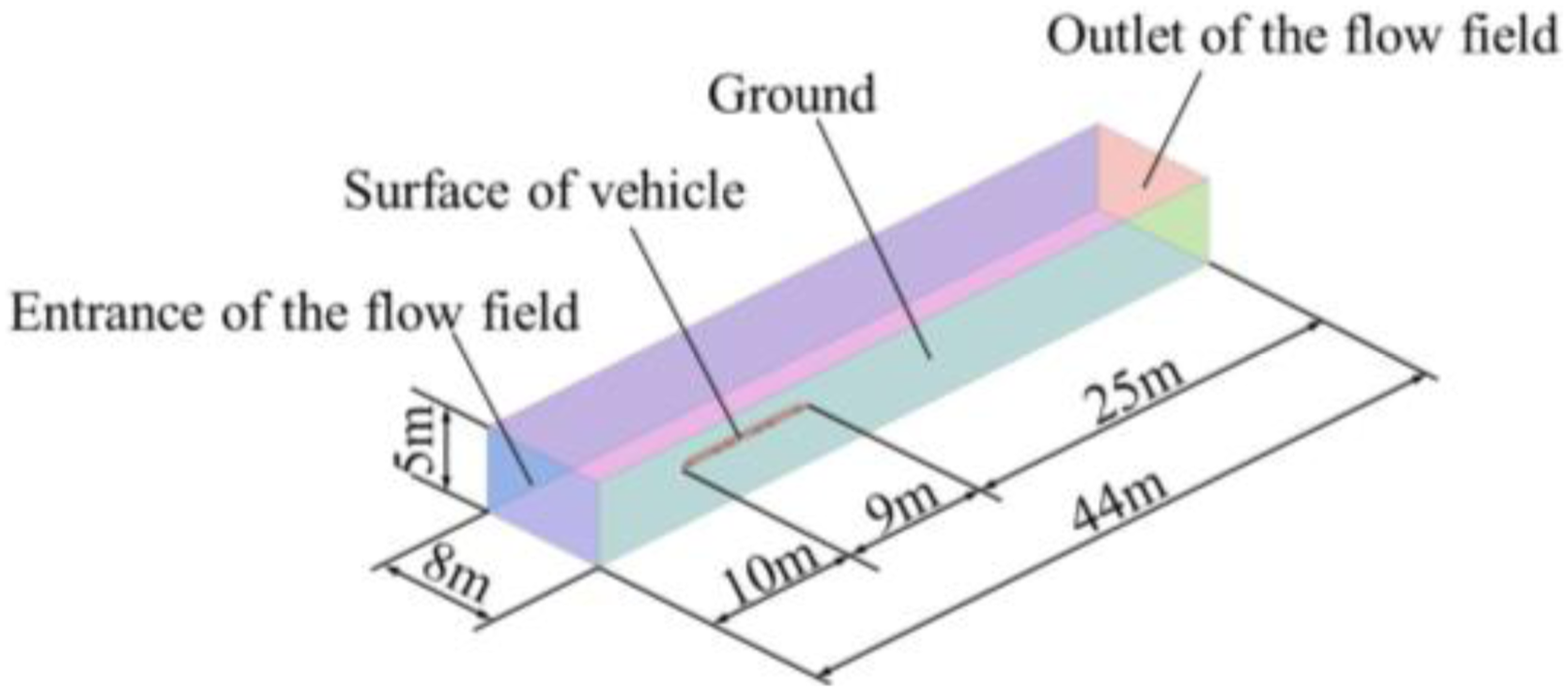

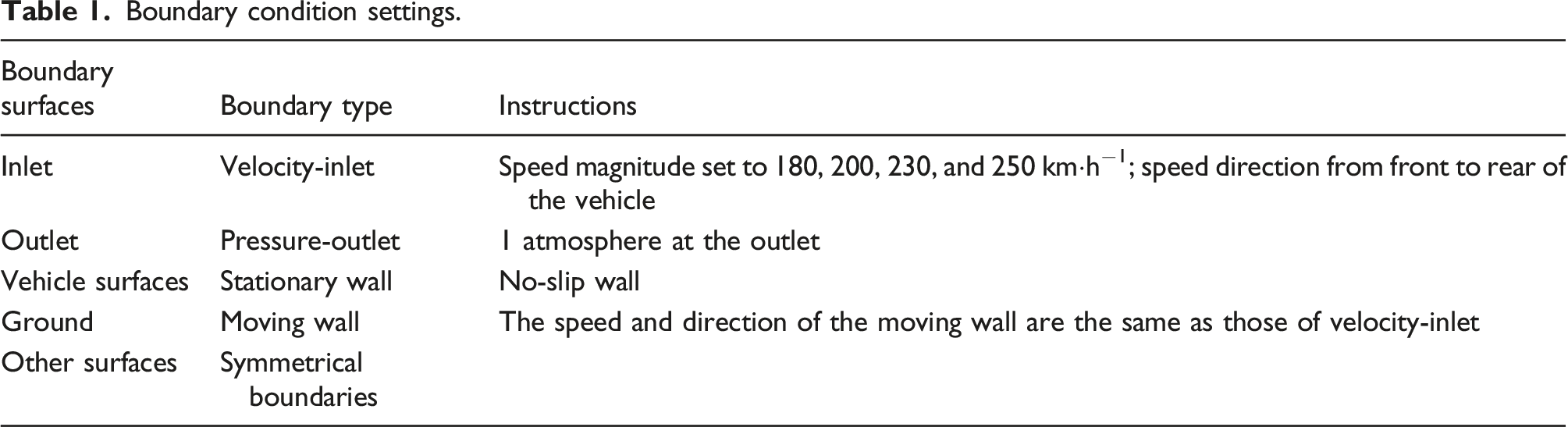
The boundary conditions are the same for the full-scale model and scale-down model. Assuming the vehicle is stationary, the fluid simulates the actual motion of the vehicle at the magnitude of the actual motion of vehicle, along the opposite direction of the vehicle’s motion. The specific settings are shown in Table 1.

Table 1.

Boundary condition settings.

Boundary surfaces	Boundary type	Instructions
Inlet	Velocity-inlet	Speed magnitude set to 180, 200, 230, and 250 km·h⁻¹; speed direction from front to rear of the vehicle
Outlet	Pressure-outlet	1 atmosphere at the outlet
Vehicle surfaces	Stationary wall	No-slip wall
Ground	Moving wall	The speed and direction of the moving wall are the same as those of velocity-inlet
Other surfaces	Symmetrical boundaries

Steady state calculations are set to the Standard $k - ε$ turbulence model. Transient calculations are performed using large eddy simulations (LES) with the steady state results as initial values. The time step is set as $Δ t = 0.0001 s$ , the number of time steps is 3000 and the total calculation time is 0.3 s.

Mesh division and independence test

Unstructured meshes are used for the flow field. Tetrahedral meshes are used for the near field, pentahedral meshes are used for the transition area between the near and far field, and hexahedral meshes are used for the far field. Due to the complex structure of the head vehicle, pantograph and bogies, which are prone to generate large noise, the meshes of these parts are encrypted.

To reduce the influence of the number of meshes on the accuracy of the numerical simulation, meshes independence test was carried out. For the scale-down model, five groups of meshes with different densities and numbers were created. Set A-weighted SPL at two receivers at 250 km·h⁻¹, with cross-sections of 1/3 and 2/3 of the vehicle length, at a distance of 7.5 m from the centerline of the vehicle and a height of 0.8 m, as the inspection standard. The comparison results are presented in Table 2.

Table 2.

Meshes independence test for scale-down model.

Number of meshes/million	Minimum mesh size/mm	SPL at 1/3 of vehicle length/dBA	SPL at 2/3 of vehicle length/dBA
14.23	6.72	83.37	82.16
18.88	6.41	78.93	78.11
22.85	5.98	78.48	77.98
29.80	5.74	78.47	77.99
36.54	5.35	78.45	78.04

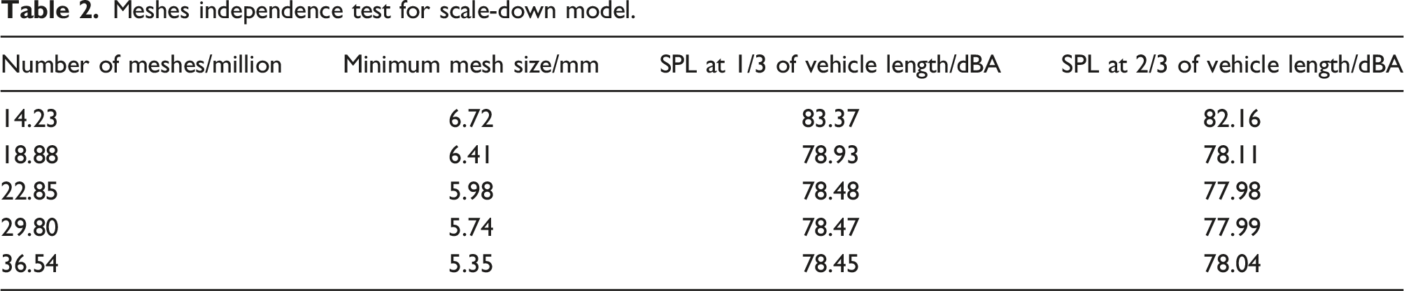
The above table indicates that SPL is basically stable at about 78dBA as the number of meshes increases, starting from 22.85 million meshes. Considering the calculation accuracy and simulation time, the 29.80 million meshes were used for numerical simulation. Set seven layers of boundary layer meshes, and normal growth rate is 1.1. In the high $R e$ number model, y+ was taken as 30. The thickness of the first layer of the meshes was calculated to be 0.32–0.44 mm at 180–250 km·h⁻¹, and set uniformly to 0.44 mm. The meshes of the scale-down model are shown in Figure 4.

Figure 4.

Meshes for the scale-down model. (a) Local flow field, (b) boundary layer, (c) the front of the vehicle, (d) bogies.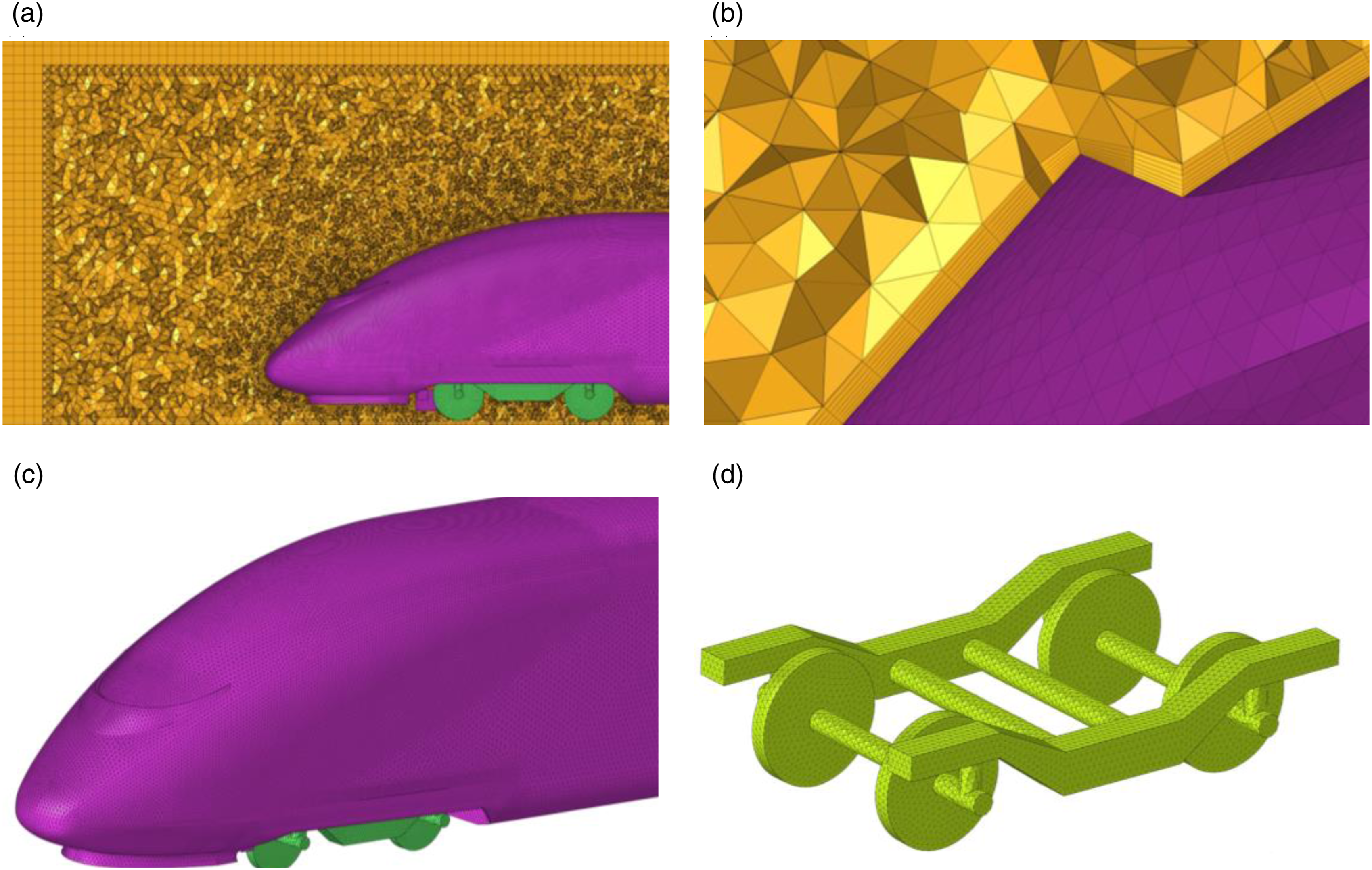

For the mesh independence test of the full-scale model, five groups of meshes with different densities and numbers are divided. The coordinates of the monitoring points of the full-scale model at 250 km·h⁻¹ are 8 times of the scale-down model, which means the cross-sections at 1/3 and 2/3 of the length of the vehicle, 60 m from the centerline of the vehicle body and 6.4 m high. The A-weighted SPL at the two receivers was set as the test standard, and the comparison is shown in Table 3.

Table 3.

Meshes independence test for full-scale model.

Number of meshes/million	Minimum mesh size/mm	SPL at 1/3 of vehicle length/dBA	SPL at 2/3 of vehicle length/dBA
21.84	56	90.45	89.05
26.40	52	86.61	84.77
33.53	48	84.66	83.76
39.80	44	84.66	83.74
46.54	40	84.65	83.76

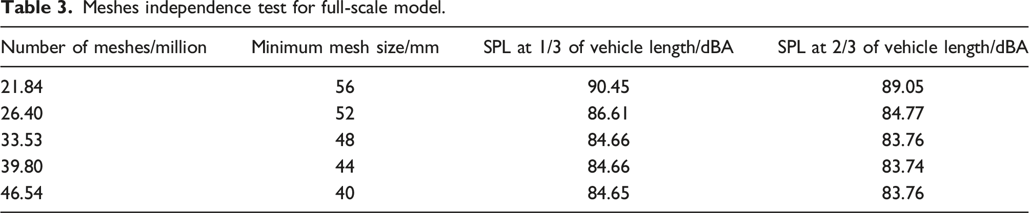
When the number of meshes is higher than 33.53 million, the change of SPL is basically stable. Considering the calculation accuracy and simulation time, 33.53 million meshes are used for numerical simulation. The minimum mesh scale of the full-scale model is 48 mm, with a total of 33.53 million meshes. Seven boundary layers are set up, the growth rate is 1.1, y+ is taken as 30, and the thickness of the first mesh layer is 0.36 mm.

Prediction of aerodynamic noise among different velocities

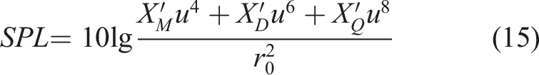
For the 1:8 scale-down complete vehicle model (including the vehicle body and bogies), aerodynamic noise at different velocities is predicted based on the line source SPL calculation formula. The predicted values will be compared with the simulated values to verify the accuracy of equation (15) in predicting the SPL at the specified velocity of the same model when the complete vehicle is used as the noise source.

Receivers settings and simulation results analysis

At a distance of 7.5 m on the same side of the vehicle centerline, with a longitudinal spacing of 3 m and a distance of 0.8 m from the ground, four receivers are set up, as shown in Figure 5.

Figure 5.

Far-field receivers location. (a) Front view, (b) left view.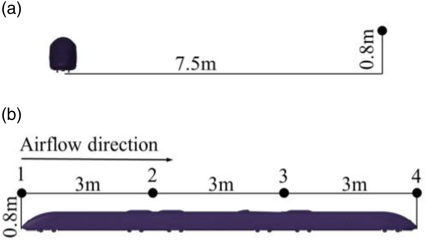

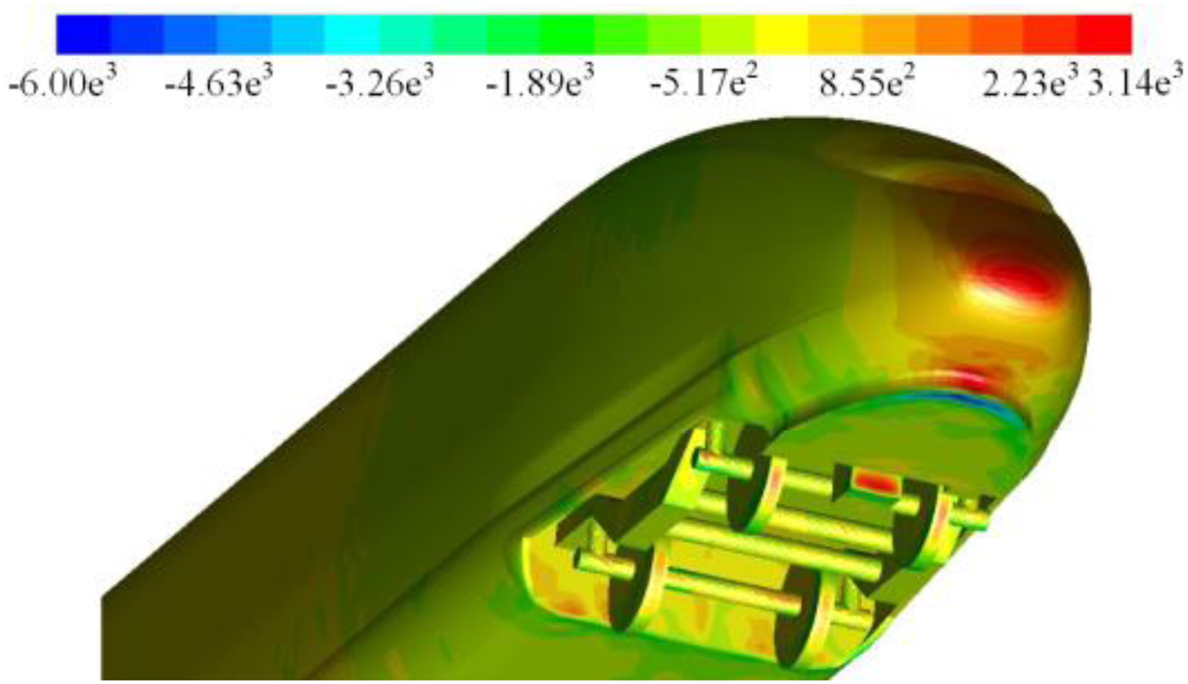
The steady state calculation obtains the surface pressure distribution of scale-down model as shown in Figure 6 (taking 250 km·h⁻¹ working condition as an example). According to Figure 6(a), the pressure at the front and rear of the vehicle is smaller relative to the middle of the vehicle. According to Figure 6(b)–(d), the surface pressure at the nose of the front end, the windward side of the bogie, and the windward side of the roof air conditioner are larger, with a maximum of 3.02 e³ Pa, and the surface pressure along the direction of the airflow will decrease rapidly, and then rebound slightly.

Figure 6.

Surface pressure distribution of scale-down model. (a) complete vehicle, (b) front end of a vehicle, (c) first bogie of the head vehicle, (d) roof air conditioner.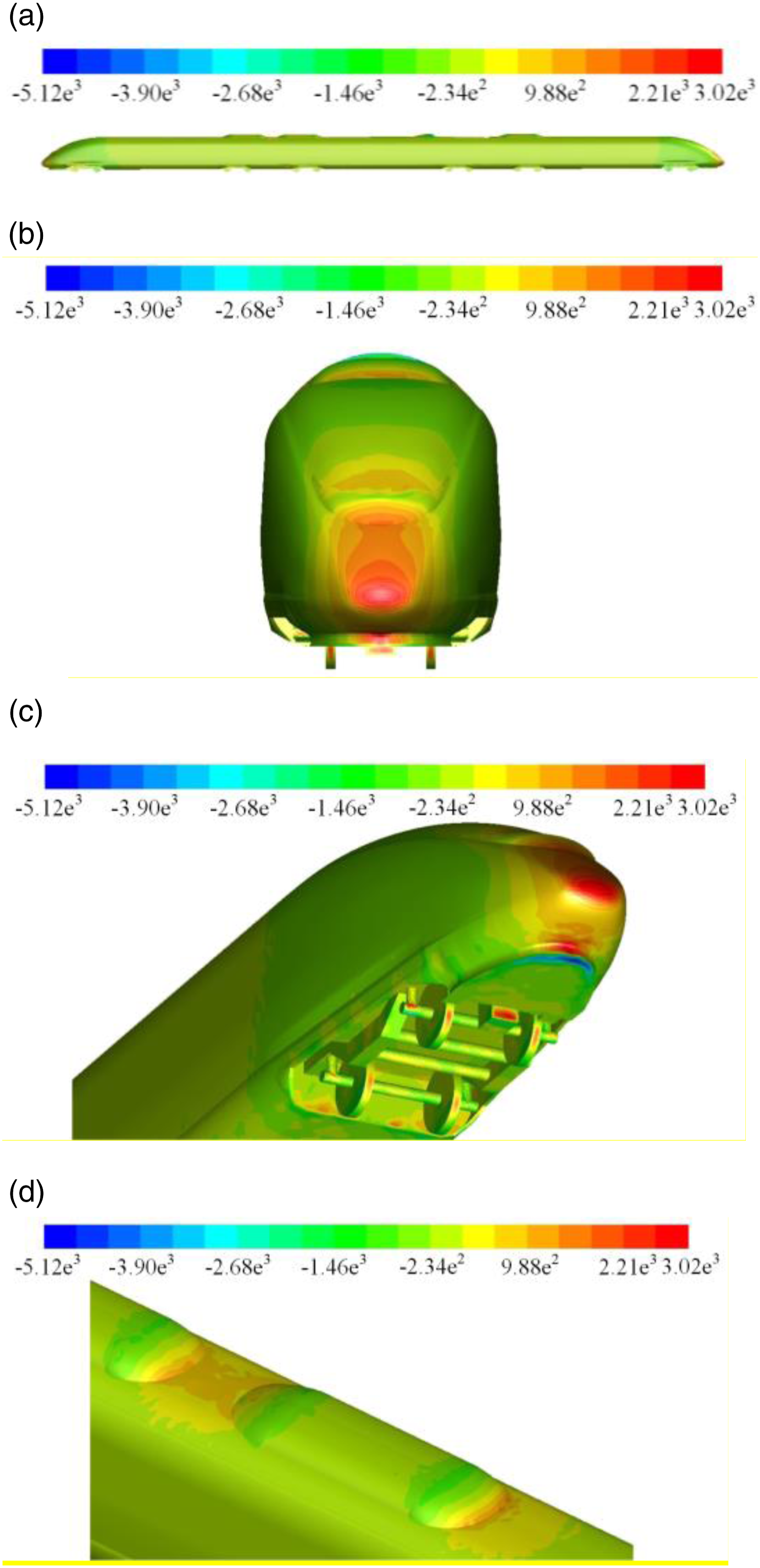

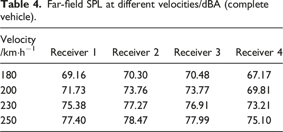
The SPL of each receiver at different velocities is shown in Table 4. The trend of SPL at each receiver under different velocities is shown in Figure 7.

Table 4.

Far-field SPL at different velocities/dBA (complete vehicle).

Velocity/km·h⁻¹	Receiver 1	Receiver 2	Receiver 3	Receiver 4
180	69.16	70.30	70.48	67.17
200	71.73	73.76	73.77	69.81
230	75.38	77.27	76.91	73.21
250	77.40	78.47	77.99	75.10

Figure 7.

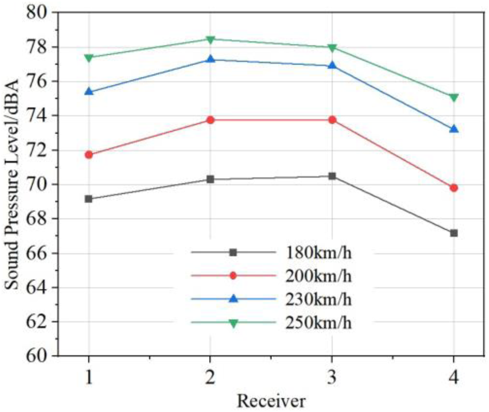
SPL trend of each receiver at different velocities.

The above table and the figure shows that, SPL values at receiver 1 and 4, which are flush with the front and rear of the vehicle, are significantly smaller than those at receiver 2 and 3 at the same velocity, while SPL values at receiver 2 and 3 do not differ significantly. The speed does not affect the variation rule of the total SPL along the centerline of vehicle. The 1/3-octave SPL spectra of each receiver at different speeds is shown in Figure 8.

Figure 8.

1/3-octave A-weighted spectra. (a) receiver 1, (b) receiver 2, (c) receiver 3, (d) receiver 4.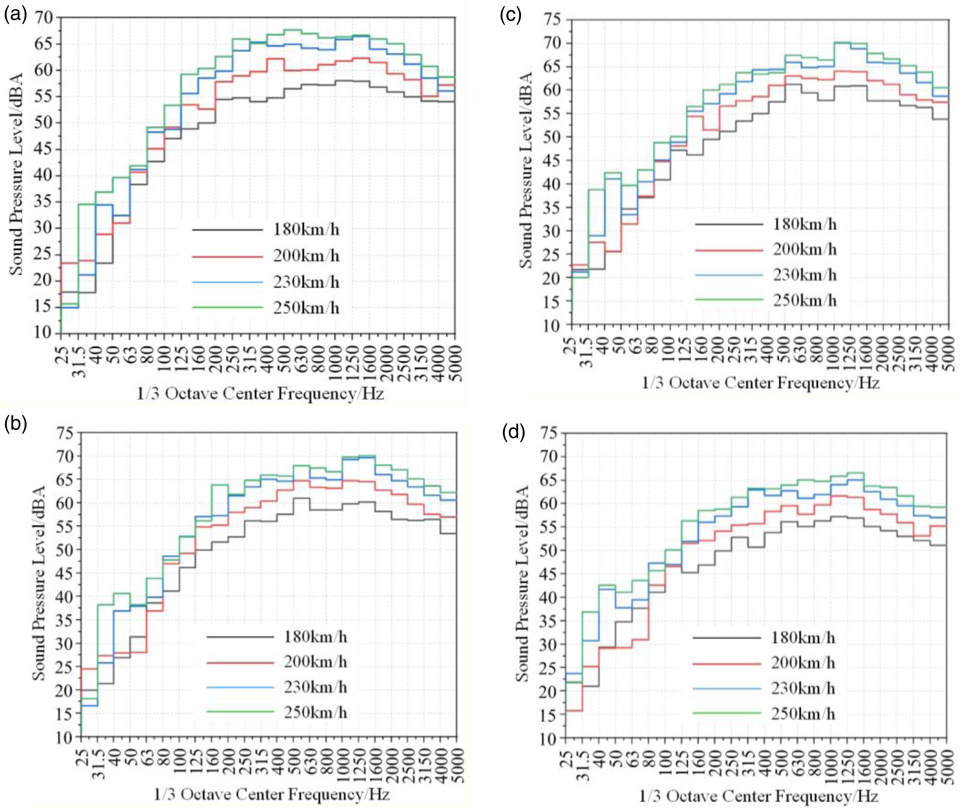

The above figure shows that aerodynamic noise exists over a wide frequency domain, and SPL in the range of 200–5000 Hz contributes the most to the total SPL. When the frequency reaches 1250 Hz, SPL peaks and starts to decrease. In the range of 200–5000 Hz, there is not much difference between the increase and decrease of SPL, while the increase of SPL below 200 Hz is significant. In addition, the speed and the location of the receiver do not affect the trend of SPL with frequency.

High-speed aerodynamic noise prediction using low-speed state simulation values

Based on equation (15), the noise data at 180, 200 and 230 km·h⁻¹ at the same receiver is used to calculate the undetermined coefficients, and the undetermined coefficients are used to predict SPL of that receiver at 250 km·h⁻¹. In this part of the research work, it has been ensured that the similar parameters of the scale-down model for the four velocity conditions satisfy the similarity criterion (geometrical similarity, $M a$ number similarity, $R e$ number similarity), and therefore the subsequent prediction work can be carried out. $r_{0} = \sqrt{7 . 5^{2} + {(0.8 - 0.25)}^{2}} = 7.52$ m at the four velocities (setting the vehicle centerline height at 0.25 m) referring to Figure 1. Taking receiver 1 as an example, the SPL calculation equations for the four velocities are listed below ( $u$ has been converted to m·s⁻¹).

69.16 = 10 \lg \frac{50^{4} X_{M} + 50^{6} X_{D} + 50^{8} X_{Q}}{{7.52}^{2}}

(19)

71.73 = 10 \lg \frac{{55.56}^{4} X_{M} + {55.56}^{6} X_{D} + {55.56}^{8} X_{Q}}{{7.52}^{2}}

(20)

75.38 = 10 \lg \frac{{63.89}^{4} X_{M} + {63.89}^{6} X_{D} + {63.89}^{8} X_{Q}}{{7.52}^{2}}

(21)

L_{P} = 10 \lg \frac{{69.44}^{4} X_{M} + {69.44}^{6} X_{D} + {69.44}^{8} X_{Q}}{{7.52}^{2}}

(22)

Comparisons between the prediction results and the numerical simulation results are shown in Table 5, which show that the highest error between the two results at 250 km·h⁻¹ is only 0.28 dBA.

Table 5.

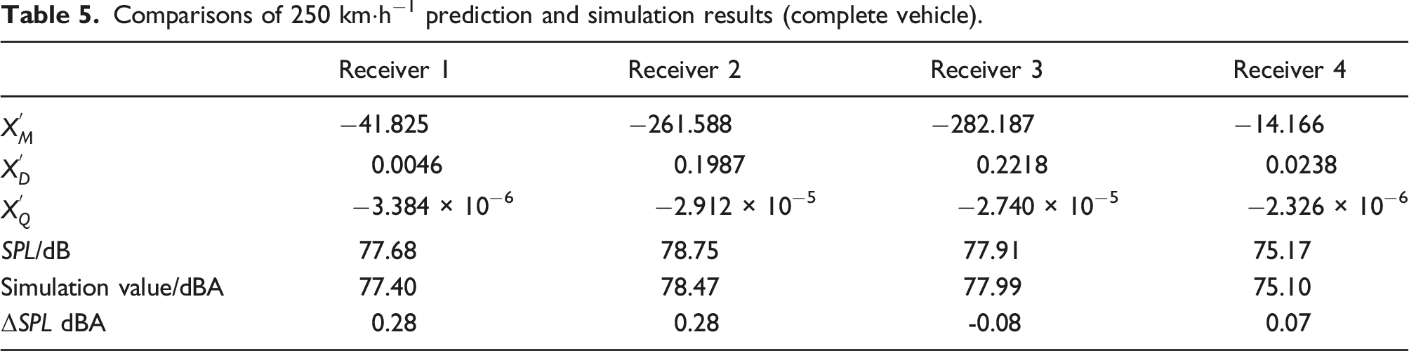
Comparisons of 250 km·h⁻¹ prediction and simulation results (complete vehicle).

	Receiver 1	Receiver 2	Receiver 3	Receiver 4
$X_{M}^{'}$	−41.825	−261.588	−282.187	−14.166
$X_{D}^{'}$	0.0046	0.1987	0.2218	0.0238
$X_{Q}^{'}$	−3.384 × 10⁻⁶	−2.912 × 10⁻⁵	−2.740 × 10⁻⁵	−2.326 × 10⁻⁶
SPL/dB	77.68	78.75	77.91	75.17
Simulation value/dBA	77.40	78.47	77.99	75.10
$Δ S P L$ dBA	0.28	0.28	-0.08	0.07

Low-speed aerodynamic noise prediction using high-speed state simulation values

Using data of 200, 230 and 250 km·h⁻¹ velocities, SPL and the undetermined coefficients for each receiver of scale-down model at 180 km·h⁻¹ is predicted by equation (15), with the variables assigned as above. Comparisons are shown in Table 6.

Table 6.

Comparisons of 180 km·h⁻¹ prediction and simulation results (complete vehicle).

	Receiver 1	Receiver 2	Receiver 3	Receiver 4
$X_{M}^{'}$	−48.557	−272.790	−253.593	−16.704
$X_{D}^{'}$	0.0056	0.2620	0.2055	0.0310
$X_{Q}^{'}$	−3.789 × 10⁻⁶	−3.094 × 10⁻⁵	−2.513 × 10⁻⁵	−2.321 × 10⁻⁶
SPL/dBA	68.95	69.98	70.57	67.08
Simulation value/dBA	69.16	70.30	70.48	67.17
$Δ S P L$ /dBA	−0.21	−0.32	0.09	−0.09

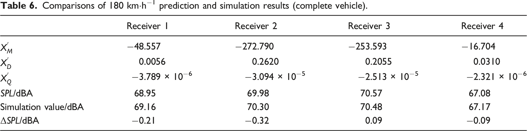
The maximum error between the predicted aerodynamic noise values for the low-speed condition and the numerical simulation results is 0.32 dBA. The results show that the aerodynamic noise calculation method in this study is accurate in predicting aerodynamic noise at different speeds for the same model.

According to Tables 5 and 6, the values of the undetermined coefficients have the following characteristics. The undetermined coefficients of dipole sources at different receivers are all positive, while those of monopole and quadrupole sources at different receivers are all negative. According to equation (16), the product function of the three undetermined coefficients is positive and the integration result is positive. Since $ρ$ , $u$ , and $c$ are positive, $k_{D}$ is positive while $k_{M}$ and $k_{Q}$ are negative.

Analysis of the pattern of change of the undetermined coefficients:

(1) The three undetermined coefficients differ significantly between different receivers. This is because according to the analysis above, there are variations in the characteristic sizes of sound sources at various points along the centerline of the vehicle, and different receivers have different distances from the sound sources to various points on the line, which in turn affects the integration results in equation (15).

(2) The undetermined coefficients of dipole sound source vary relatively smoothly in the middle of the vehicle (receiver 2 and 3), while the values in the middle of the vehicle are greater than those at both ends of the vehicle (receiver 1 and four). The trend of the undetermined coefficients of dipole sound source is similar to the trend of SPL. The tendency of the undetermined coefficients of monopole and quadrupole sources varies in the opposite direction to SPL, meaning that the values in the middle of the vehicle are smaller than those at the ends of the vehicle.

(3) The similarity of the same undetermined coefficients at the same receiver indicates that velocity does not have a significant effect on the undetermined coefficients.

High-speed aerodynamic noise prediction of local noise sources

Using the same method, far-field aerodynamic noise predictions are performed for the local noise sources (bogies). The accuracy of the prediction is verified when the first bogie of head vehicle or all bogies are used as the noise source.

The first bogie of head vehicle as a noise source

The receivers and velocity settings are the same as above, and the sound source in Fluent software was set to the first bogie of the head vehicle. The numerical simulation results are shown in Table 7. The trend of SPL changes at each receiver at different speeds is shown in Figure 9. The 1/3-octave SPL spectra at different speeds are shown in Figure 10. (take receiver 3 as an example, and the spectra of the rest of receivers are similar to it). Table 7 and Figure 9 show that SPL decreases as the distance between the receiver and the noise source increases, and increases as the speed increases. Velocity does not affect the trend of SPL along distance. Figure 10 shows that SPL at 200–1600 Hz contributes the most to the total SPL when the first bogie of the head car is used as a noise source. When the frequency increases to 315 Hz, SPL peaks and then gradually decreases, but at 1250 Hz, there is a small rebound of SPL, which then continues to decrease. Compared to the case where the whole vehicle is used as a noise source, the main frequency range leading to noise is reduced. The rise in SPL before 315 Hz is relatively large and the drop in SPL after 315 Hz is relatively small, but both the rise and the drop are more significant than the case where the whole vehicle is used as a noise source.

Table 7.

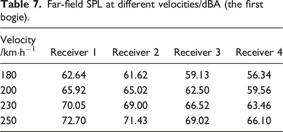
Far-field SPL at different velocities/dBA (the first bogie).

Velocity/km·h⁻¹	Receiver 1	Receiver 2	Receiver 3	Receiver 4
180	62.64	61.62	59.13	56.34
200	65.92	65.02	62.50	59.56
230	70.05	69.00	66.52	63.46
250	72.70	71.43	69.02	66.10

Figure 9.

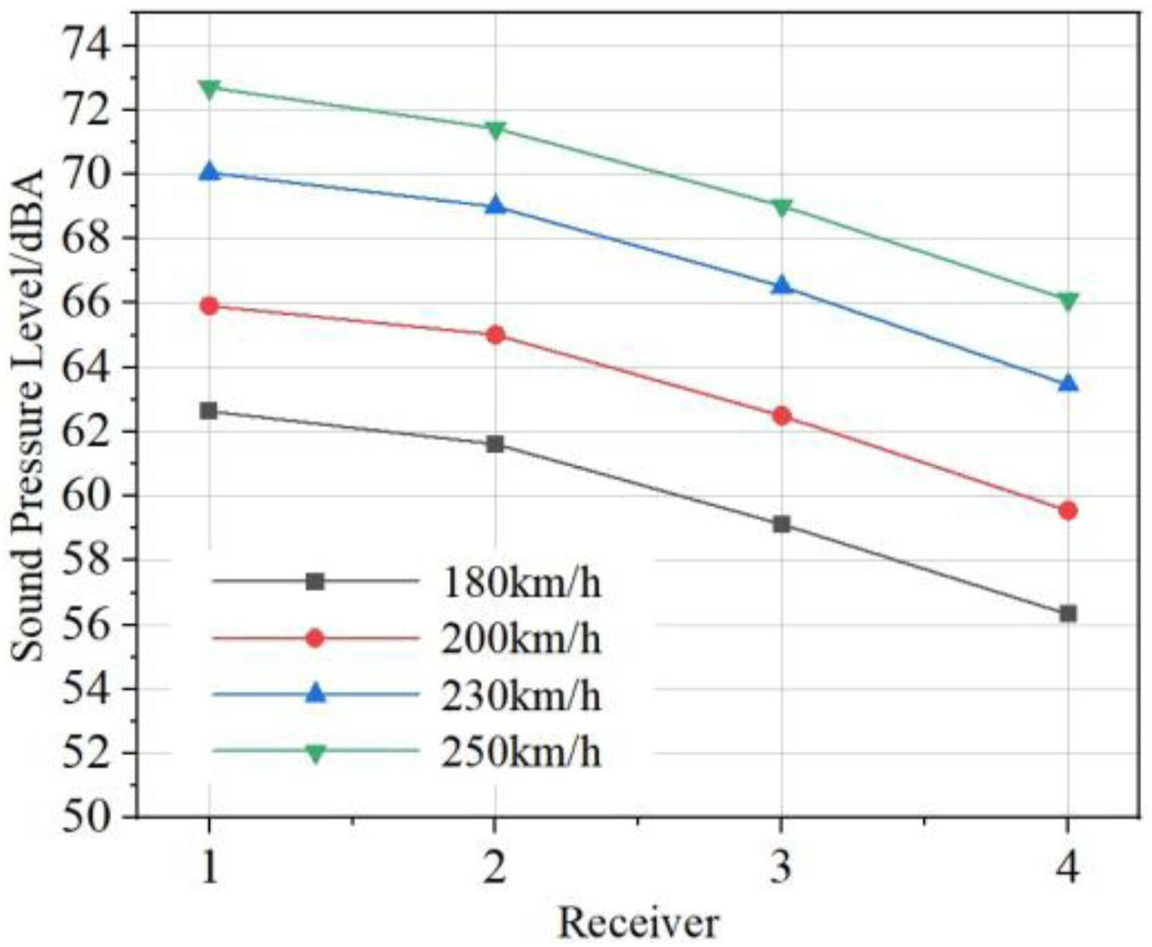
Trend of SPL (the first bogie).

Figure 10.

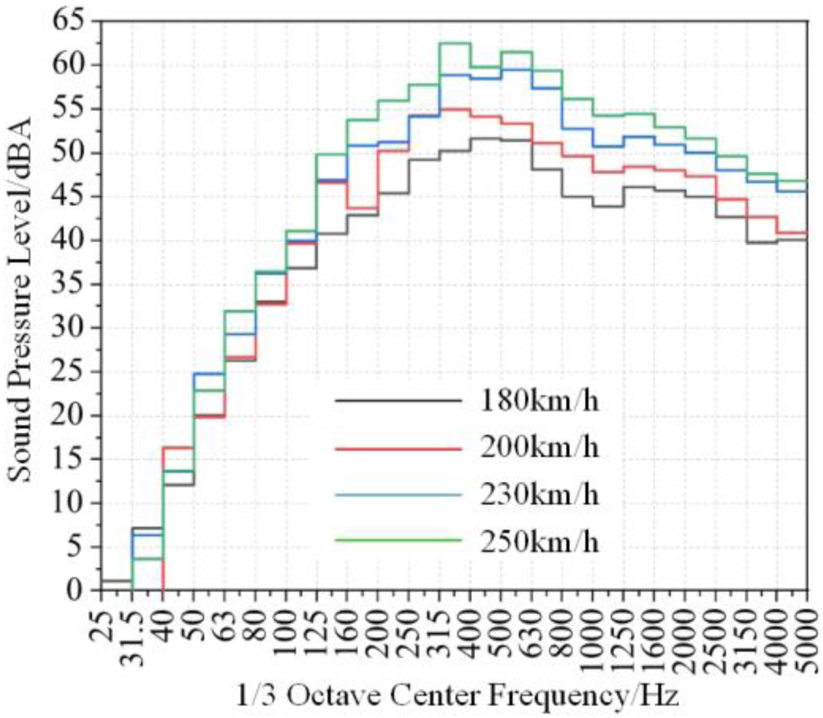
1/3-octave A-weighted spectra at receiver 3 (the first bogie).

The first bogie is considered as a point noise source, and the distance between each receiver and the center of the bogie is calculated. Using equation (9), the data of the first three velocities in the above table are used as known to predict SPL at each receiver of the scale-down model at 250 km·h⁻¹ after deriving the undetermined coefficients. Comparisons of predicted and simulated results are shown in Table 8. The prediction work in this section still satisfies the similarity criteria.

Table 8.

Comparisons of 250 km·h⁻¹ prediction and simulation results (the first bogie).

	Receiver 1	Receiver 2	Receiver 3	Receiver 4
$X_{M}$	−19.587	−18.977	−14.057	−8.880
$X_{D}$	0.0214	0.0170	0.0117	0.0082
$X_{Q}$	−8.511 × 10⁻⁶	−1.112 × 10⁻⁶	−6.382 × 10⁻⁷	−4.618 × 10⁻⁷
$S P L$ /dBA	72.43	71.15	68.73	65.92
Simulation value/dBA	72.70	71.43	69.02	66.10
$Δ S P L$ /dBA	−0.27	−0.28	−0.29	−0.18

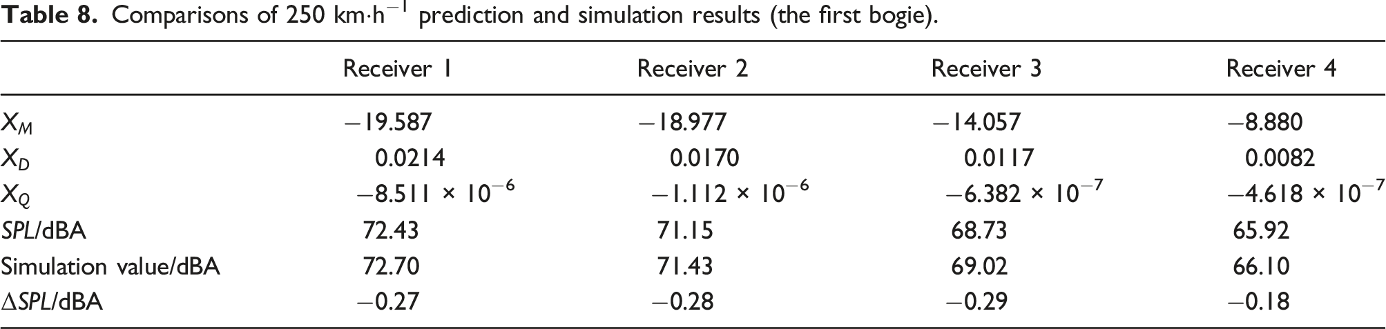
The above table shows that when the first bogie of head vehicle is used as a local noise source, the maximum error between the predicted and simulated values at each receiver is 0.28 dBA, which is a relatively accurate prediction.

As the distance between the receiver and the sound source increases, the undetermined coefficients of dipole sources gradually decrease, with the same pattern of variation as SPL, while the undetermined coefficients of monopole and quadrupole sources gradually increase. The distance-dependent characteristic of the undetermined coefficients is because the main part of the noise generated by the bogie is in frontal contact with the airflow, which is the area in the negative direction of the x-axis with respect to the center of the bogie (refer to Figure 1). When the receiver moves along the direction of the airflow (forward of the x-axis), the area where the bogie is in frontal contact with the airflow becomes difficult to effect for more distant receivers. Even if the entire bogie area is considered as a single point, the characteristic size of the three sources at this point will vary with distance, which in turn affect the variation of the undetermined coefficients. However, as the key areas of noise emitted by the bogie have a similar effect at the same receiver, it is more accurate to use the same receiver for prediction.

All bogies as noise source

The six bogies of the three vehicles are used as a noise source, and the receivers and speed settings remain unchanged. As the impact of the noise generation area on each bogie is different for each receiver, this means that each bogie has different characteristic sizes for the three sources. If all bogies are considered as six point noise sources and each point source contains three undetermined coefficients in equation (9), equation (9) will contain a total of 18 undetermined coefficients based on the principle of sound intensity superposition, which is difficult to solve and requires 18 sets of data at different velocities. To simplify the calculation, all bogies are considered as a line source. The location of the line source is the line connecting the bogie centers.

Using equation (15), SPL of the scale-down bogie model at 250 km·h⁻¹ is predicted after calculating the distance between the receivers and the line source (

r_{0}

). The results of the numerical calculations at 250 km·h⁻¹ are shown in Table 9. The trend of SPL changes is shown in Figure 11, and the 1/3-octave SPL spectrum is shown in Figure 12 (with receiver 3 as an example). As can be seen from Table 9 and Figure 11, SPL is larger at the receiver near the first bogie, and gradually decreases from the front to the back. For receiver 1, the difference between the noise generated by all bogies and by the first bogie is very small (0.29 dBA). As the distance of the receiver increases, SPL gradually decreases, but the decrease is relatively flat compared to the case where the first bogie is the noise source. Figure 12 shows that when the frequency gradually increases, SPL increases until it peaks at 500 Hz. Then SPL starts to decrease, but there is a small rebound at 1250 Hz and then continues to decrease. The comparisons between predictions and simulations are shown in Table 10.

Table 9.

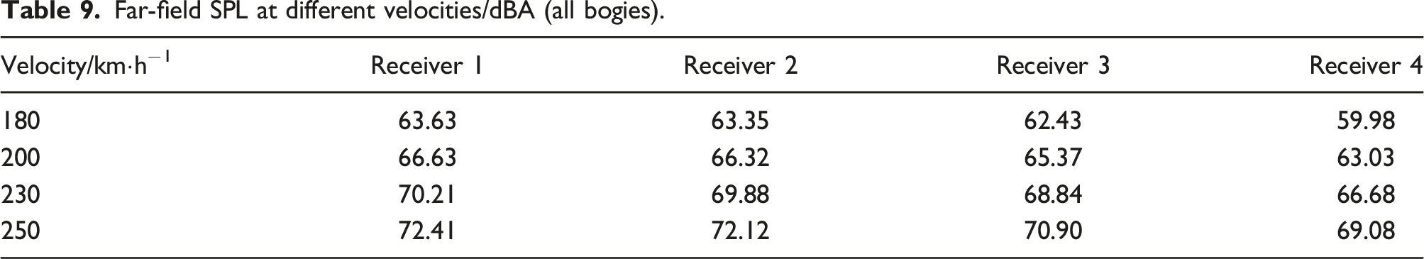
Far-field SPL at different velocities/dBA (all bogies).

Velocity/km·h⁻¹	Receiver 1	Receiver 2	Receiver 3	Receiver 4
180	63.63	63.35	62.43	59.98
200	66.63	66.32	65.37	63.03
230	70.21	69.88	68.84	66.68
250	72.41	72.12	70.90	69.08

Figure 11.

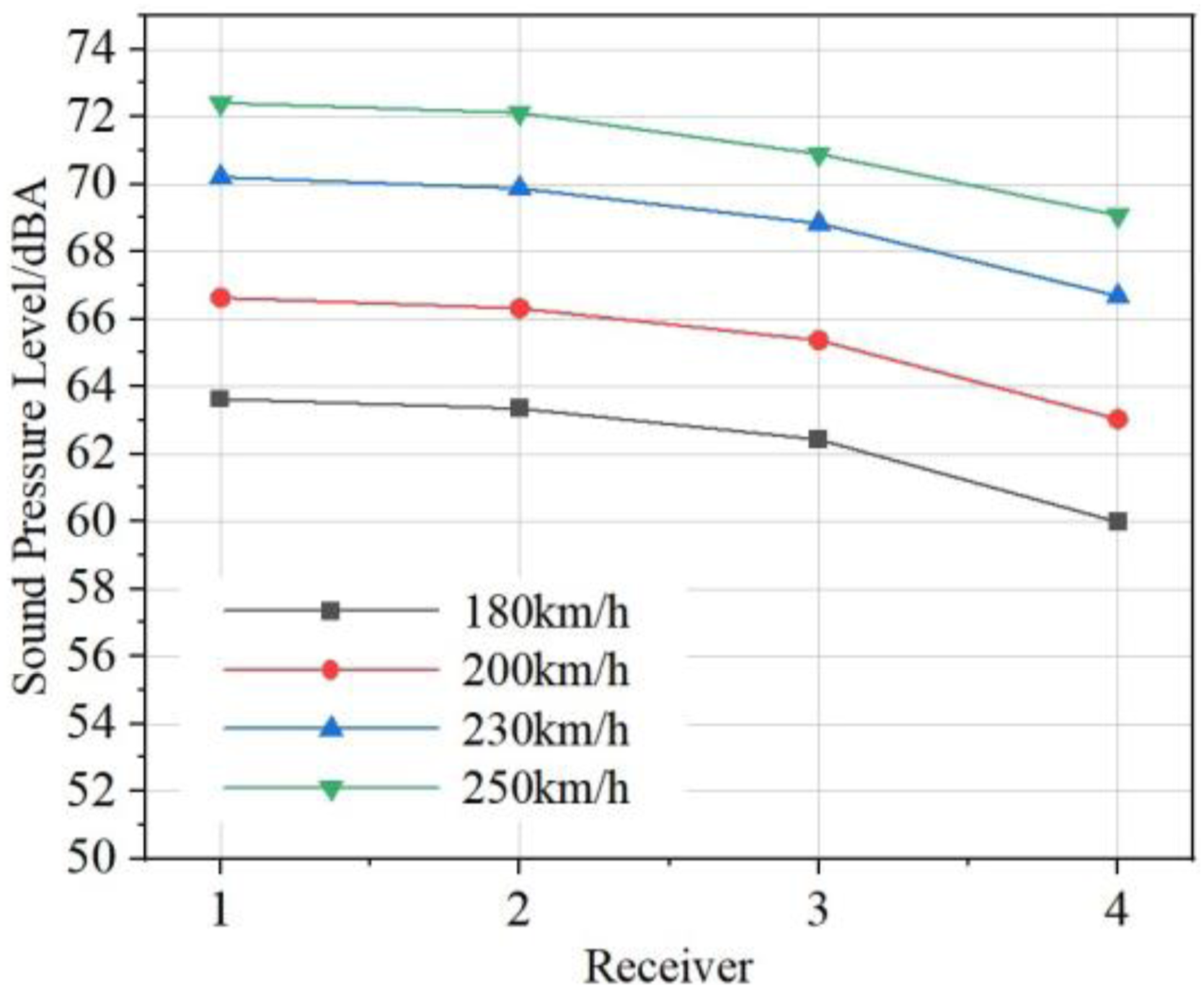
Trend of SPL (all bogies).

Figure 12.

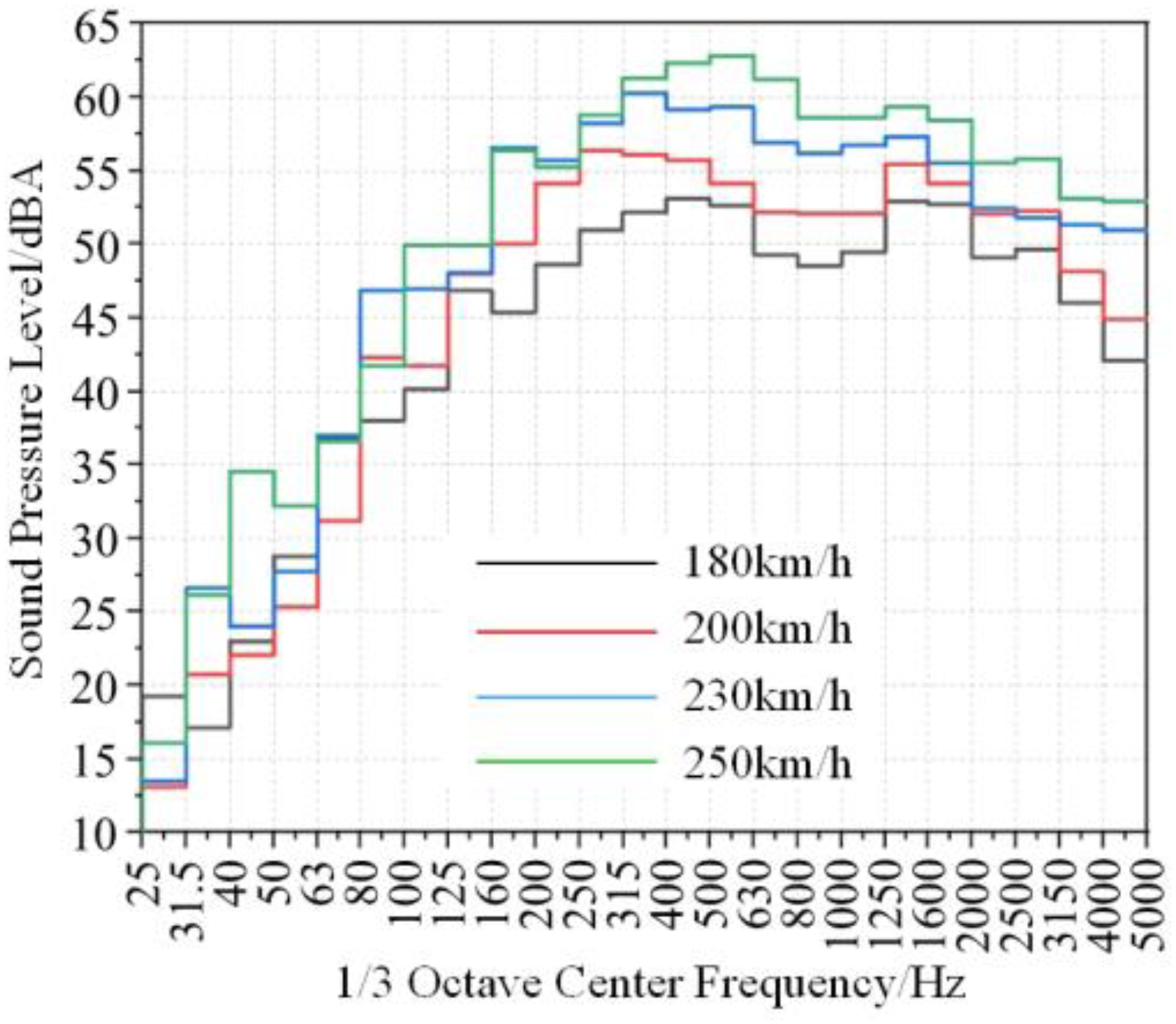
1/3-octave A-weighted spectra at receiver 3 (all bogies).

Table 10.

Comparisons of 250 km·h⁻¹ prediction and simulation results (all bogies).

	Receiver 1	Receiver 2	Receiver 3	Receiver 4
$X_{M}^{'}$	−19.394	−16.977	−14.830	−3.991
$X_{D}^{'}$	0.0203	0.0184	0.0158	0.0058
$X_{Q}^{'}$	−1.662 × 10⁻⁶	−1.499 × 10⁻⁶	−1.433 × 10⁻⁶	−2.174 × 10⁻⁷
$S P L$ /dBA	72.12	71.79	70.58	68.94
Simulation value/dBA	72.41	72.12	70.90	69.08
$Δ S P L$ /dBA	−0.29	−0.33	−0.32	−0.14

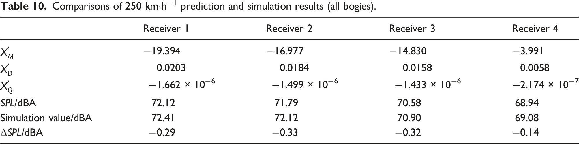
The table above shows that the maximum error between the predicted and simulated values is 0.33 dBA for the six bogies as a noise source. The variation pattern of the undetermined coefficients of dipole source with the location of receivers is similar to that of the aerodynamic noise generated by the six bogies, meaning that SPL and the undetermined coefficients of dipole sources are higher at the receiver near the first bogie and gradually decrease from front to back. The variation pattern of the undetermined coefficients of monopole and quadrupole sources is the opposite of that of dipole sources. The undetermined coefficients of dipole sources are positive, while those of monopole and quadrupole sources are negative. The above work further validates the high accuracy of the local noise source prediction.

Prediction of aerodynamic noise of full-scale model by scale-down model

It is more practical to reduce the workload and improve the efficiency of the calculation by using the scale-down model simulation data to predict the aerodynamic noise of the full-scale vehicle body based on equation (15).

The layout of the scale-down model receivers is the same as above. The coordinates of the full-scale model receivers are 8 times larger than that of scale-down model receivers, meaning that four receivers are set at 24 m intervals, 60 m from the same side of the vehicle centerline and 6.4 m from the ground. The numerical simulation results of the full-scale model at 250 km·h⁻¹ are shown in Table 11. The pressure distribution on the surface of the full-scale model is shown in Figure 13. As can be seen from Figure 13, the pressure distribution of the full-scale model is similar to that of the scale-down model in Figure 6(c). The maximum pressure is 3.14 e³ Pa, which is slightly higher than that of the scale-down model. The spectrograms of SPL and 1/3-octave A-weighted spectra of the scale-down model and full-scale model at receiver 3 are shown in Figures 14 and 15. As can be seen from the figures, the spectrograms of scale-down model and full-scale model are similar in that the overall SPL decreases slowly with the increase of frequency. The maximum SPL occurs at 44.87 Hz for the scale-down model at 68.30 dB. The maximum SPL occurs at 16.23 Hz for the full-scale model, at 71.88 dB. In addition, SPL span of the full-scale model is significantly larger than that of the scale-down model. According to Figure 15, the maximum contribution of SPL is found in the frequency range of 200–2000 Hz in the full-scale model. This frequency range is smaller than the main frequency range of scale-down model (200–5000 Hz). SPL rise and fall of full-scale model is larger than that of scale-down model.

Table 11.

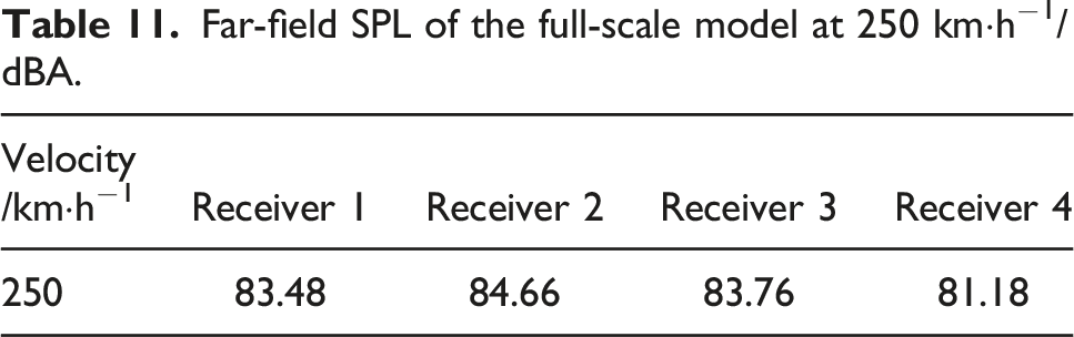
Far-field SPL of the full-scale model at 250 km·h⁻¹/dBA.

Velocity/km·h⁻¹	Receiver 1	Receiver 2	Receiver 3	Receiver 4
250	83.48	84.66	83.76	81.18

Figure 13.

Full-scale model surface pressure distribution.

Figure 14.

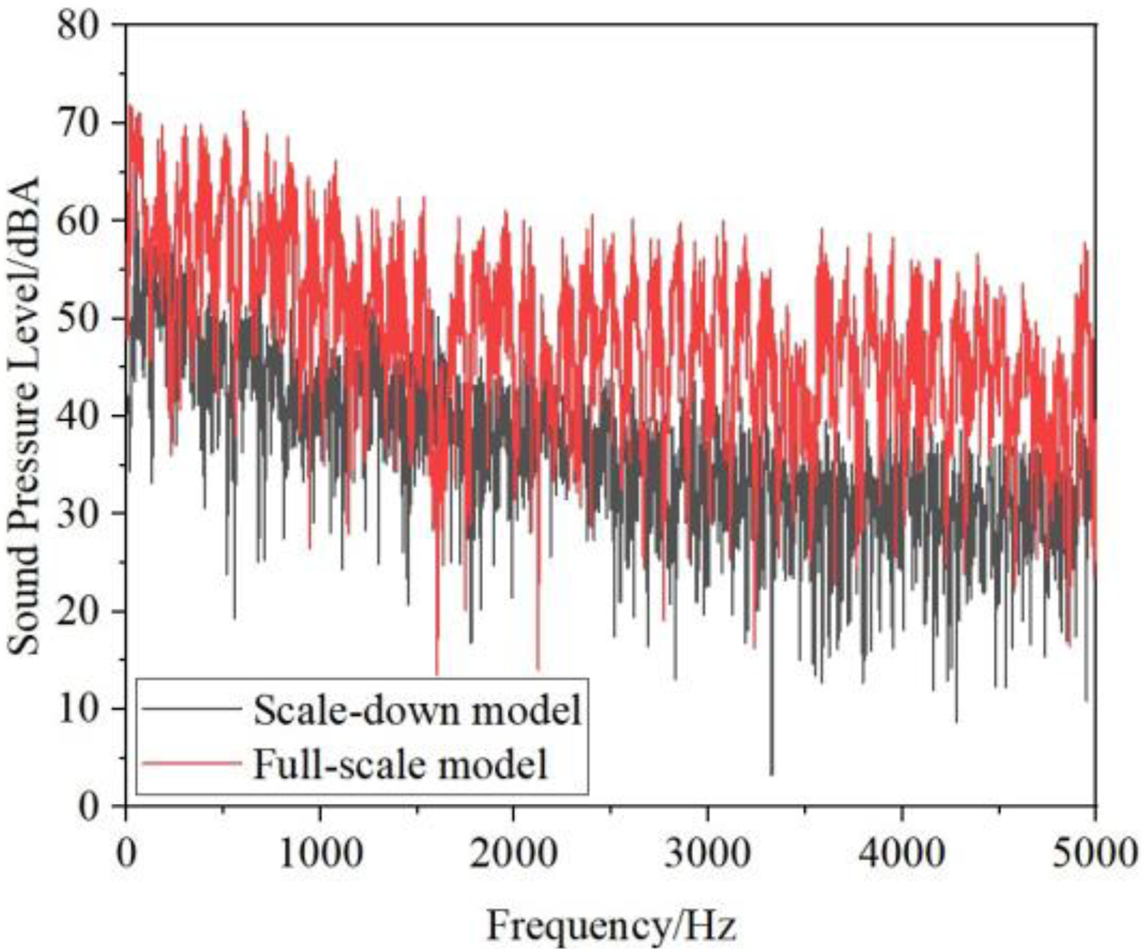
Spectrogram of SPL at receiver 3 (scale-down model and full-scale model).

Figure 15.

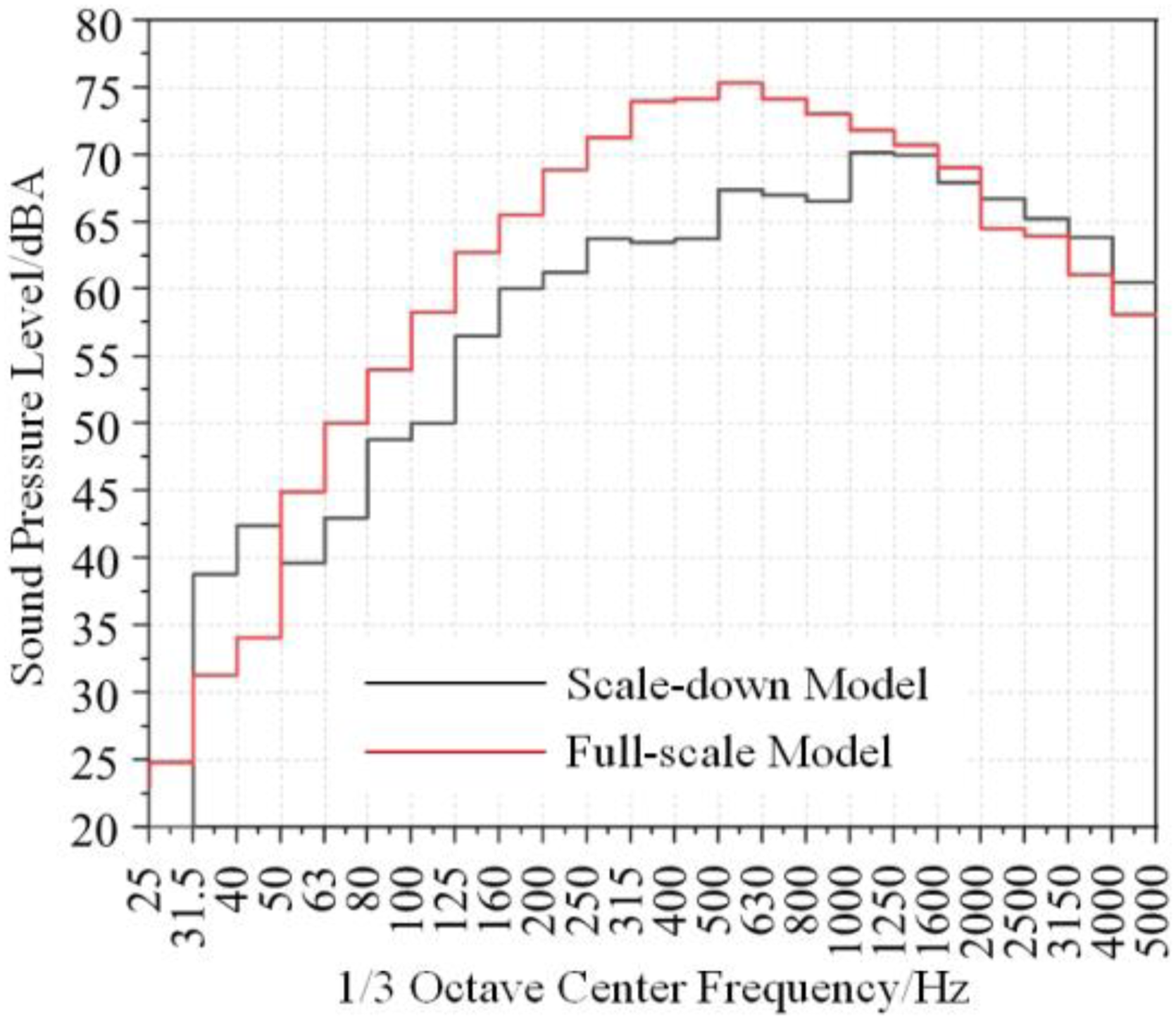
1/3-octave A-weighted spectra at receiver 3 (scale-down model and full-scale model).

According to the analysis above, the three undetermined coefficients are generally constant at the same receiver and the same noise source. However, the size of the full-scale vehicle body and the location of the receivers vary considerably compared to the scale-down model, resulting in changes to the undetermined coefficients, so the undetermined coefficients need to be analyzed. In equation (15), the 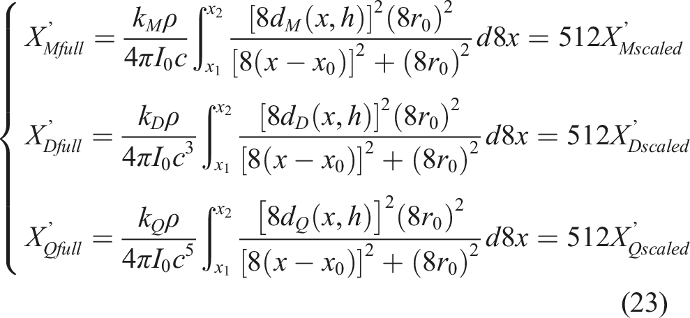$d (x, h)$ , $r_{0}$ , $x_{0}$ , and $x$ of the full-scale model are 8 times larger than those of the scale-down model (without considering the change in the upper and lower limits of integration, and directly expanding the integration variable $x$ by a factor of 8 to facilitate analytical calculations), then the undetermined coefficients of the scale-down model and the full-scale model are related as follows.

{\begin{cases} X_{M f u l l}^{'} = \frac{k_{M} ρ}{4 π I_{0} c} \int_{x_{1}}^{x_{2}} \frac{{[8 d_{M} (x, h)]}^{2} {(8 r_{0})}^{2}}{{[8 (x - x_{0})]}^{2} + {(8 r_{0})}^{2}} d 8 x = 512 X_{M s c a l e d}^{'} \\ X_{D f u l l}^{'} = \frac{k_{D} ρ}{4 π I_{0} c^{3}} \int_{x_{1}}^{x_{2}} \frac{{[8 d_{D} (x, h)]}^{2} {(8 r_{0})}^{2}}{{[8 (x - x_{0})]}^{2} + {(8 r_{0})}^{2}} d 8 x = 512 X_{D s c a l e d}^{'} \\ X_{Q f u l l}^{'} = \frac{k_{Q} ρ}{4 π I_{0} c^{5}} \int_{x_{1}}^{x_{2}} \frac{{[8 d_{Q} (x, h)]}^{2} {(8 r_{0})}^{2}}{{[8 (x - x_{0})]}^{2} + {(8 r_{0})}^{2}} d 8 x = 512 X_{Q s c a l e d}^{'} \end{cases}

(23)

The data of the scale-down model at 180, 200 and 230 km·h⁻¹ were used to calculate the undetermined coefficients by using equation (15). The SPL at the receivers for the full-scale model at 250 km·h⁻¹ were predicted by expanding the undetermined coefficients of scale-down model by a factor of 512. Predictions need to satisfy the geometrical similarity,

M a

number similarity and

R e

number similarity criteria. The most important of these is that the

R e

numbers of the scale-down model the full-scale model must be in the self-simulation region, otherwise no prediction can be made. Comparisons of predicted and simulated results is shown in Table 12.

Table 12.

SPL comparisons of full-scale model at 250 km·h⁻¹.

	Receiver 1	Receiver 2	Receiver 3	Receiver 4
$X_{M f u l l}^{'}$	−1070.723	−6696.641	−7224.015	−1476.545
$X_{D f u l l}^{'}$	1.1872	50.8691	56.7816	6.3686
$X_{Q f u l l}^{'}$	−8.663 × 10⁻⁴	−0.0057	−0.0070	−3.796 × 10⁻⁴
$S P L$ /dBA	83.71	84.77	83.93	81.18
Simulation value/dBA	83.48	84.66	83.76	81.18
$Δ S P L$ /dBA	0.23	0.11	0.17	0.00

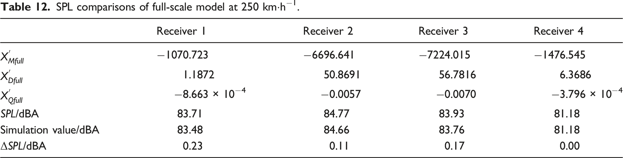
The above table shows that the maximum error between the predicted and simulated values is 0.23 dBA, which means that the predicted results are relatively accurate.

Discussion

For the numerical calculation results of SPL of the scale-down model at 250 km·h⁻¹, with the increase of the number of meshes, SPL is basically stable from 22.85 million meshes onwards, which is about 78 dBA (shown in Table 2). Compared with the simulation results of related study (SPL at the receiver at 2/3 of the vehicle length in a 1:8 scale-down 3-vehicle formation high-speed train model is approximately 78.5 dBA), the difference between the data in this study and the literature is approximately 0.5 dB at the same location.¹³ Considering the difference between the two models, the difference is within the allowable range, so the calculation results of the scale-down model in this study are accurate.

According to the related study, when the whole vehicle is the noise source, the far-field aerodynamic noise starts from the first bogie and varies steadily to the last bogie, while the noise at the front and rear of the vehicle decreases significantly.¹⁶ The change rule of SPL at different speeds in the figure is the same as the conclusion of the literature. For the 1/3-octave A-weighted spectrum, SPL change of the scale-down model in the literature²³ is consistent with the results of this paper, which means that it rises first and then slowly decreases, and the main frequencies are all 200−5000 Hz. According to literature,²⁴ the maximum surface pressure of the full-scale high-speed train with 3-vehicle formation is 3.10 e³ Pa, which is similar to the maximum pressure of the full-scale model (3.14 e³) in this paper. All these prove the accuracy of the numerical simulation results in this paper.

In this paper, it is found that when one or more bogies are used as the noise source, the main sound generating part is always the first bogie at one end of the head vehicle. When the frequency increases to 1250 Hz, SPL, which is gradually decreasing, shows a small rebound and then continues to decrease. In addition, as the frequency increases, SPL of the scale-down model increases and decreases more slowly than that of the full-scale model.

For noise prediction work, several similarity criteria need to be satisfied. Geometric similarity and $M a$ number similarity can be easily satisfied. There is no need to consider $E u$ number when fluid gravity is not taken into account. $S t$ number is mostly used for prediction work considering frequencies (back-calculating the frequency of the prototype using frequency data of the model), which is not considered in this paper. While the most important similarity criterion number is the $R e$ number. It must be ensured that the known model and the model to be predicted have similar fluid flow regimes, meaning that the Reynolds number is in the self-simulation region. This allows subsequent prediction work to be carried out.

Conclusion

In this study, the relationship between the three pneumatic basic noise sources and the far-field SPL of high-speed trains is investigated, the formula for predicting the aerodynamic noise of high-speed trains is derived, and the applicability of the aerodynamic noise calculation formula is analyzed and discussed from several aspects, providing a new and feasible approach for the prediction and analysis of aerodynamic noise of high-speed trains. The conclusions are as follows.

(1) The magnitude of SPL values is related to the location of the receiver, the size of the vehicle (characteristic size, length of vehicle) and the velocity of movement.

(2) When frequency is not considered, the prediction of aerodynamic noise of high-speed trains should adhere to the geometric similarity criterion, the $M a$ number similarity criterion and the $R e$ number similarity criterion

(3) Under the conditions of the same noise source, SPL of three known velocities at a receiver can be used to predict SPL of other velocities at the same receiver by applying the aerodynamic noise prediction formula. The noise source in the prediction work can be a complete vehicle or a local sound source such as a bogie or bogies. For the prediction of SPL among models of different sizes, the proportional variation of the parameters in the undetermined coefficients can be analyzed to accurately predict SPL at the corresponding proportional receivers.

(4) The far-field aerodynamic noise of the complete vehicle varies less in the middle of the vehicle and is greater than that at the front and rear of the vehicle. When the first bogie of the head vehicle or all bogies are used as a source, SPL is higher at the receiver near the first bogie and decreases with distance. The spectrograms, and 1/3-octave A-weighted spectral properties of the scale-down model are similar to those of the full-scale model.

(5) For the prediction of the aerodynamic noise of high-speed trains with different noise sources, the undetermined coefficients of dipole sources are all positive, and its variation trend is the same as SPL. For monopole and quadrupole sources, the undetermined coefficients are negative, and the variation trend is opposite to the trend of SPL.

Footnotes

Declaration of conflicting interests

The author(s) declared no potential conflicts of interest with respect to the research, authorship, and/or publication of this article.

Funding

The author(s) disclosed receipt of the following financial support for the research, authorship, and/or publication of this article: This work was supported by the National Natural Science Foundation of China (12102076).

ORCID iD

Jun Zhang

Appendix

References

Zhao

Yang

, et al. Analysis of the near-field and far-field sound pressure generated by high-speed trains pantograph system. Appl Acoust 2020; 169: 107506.

Noh

. Numerical analysis of aerodynamic noise from pantograph in high-speed trains using lattice Boltzmann method. Adv Mech Eng 2019; 11(7): 1687814019863995.

Merino

Morata

Srivastava

, et al. Review of research on environmental noise standards/policies/guidelines and measurement methodology in high-speed rail. Noise Vib Worldw 2022; 53(9-10): 487–497.

Sun

Yao

Wei

, et al. Numerical investigation on the influence of the streamlined structures of the high-speed train’s nose on aerodynamic performances. Appl Sci 2021; 11(2): 784.

Yao

Sun

Yang

, et al. Analysis of aerodynamic noise characteristics of high-speed train pantograph with different installation bases. Appl Sci 2019; 9(11): 2332.

Wang

Huang

. Numerical investigation into characteristics of far-field aerodynamic noise radiated by inter-coach space of high-speed maglev trains. Noise Vib Worldw 2022; 53(9-10): 464–479.

Qin

Zhou

, et al. Step-by-step numerical prediction of aerodynamic noise generated by high speed trains. Chin J Mech Eng-EN 2022; 35(1): 28.

Ouyang

, et al. Coherence and reduced order analyses of flow field and aerodynamic noise for full-scale high-speed trains pantograph. Appl Acoust 2022; 193: 108777.

Sharma

. Multi-objective design optimization of locomotive nose. SAE Technical Paper, 2021.

10.

Liu

. Numerical study on the effect of high-speed train body length on aerodynamic noise. Chin J Theoret Appl Mech 2019; 51(05): 1310–1320.

11.

Zhang

Gao

, et al. Numerical simulation of aerodynamic noise characteristics of Maglev train with speed of 600 km/h. China Railway Sci 2021; 42(06): 112–121.

12.

Wang

Zhang

, et al. Identification and analysis of pneumatic noise source in bogie area of high-speed train. J Jilin Univ (Eng Technol Edit). Epub ahead of print 20 September 2022. DOI: 10.13229/j.cnki.jdxbgxb20220364.

13.

Wang

Zhu

Wang

, et al. Characteristics identification of aerodynamic noise source in bogie area of high-speed train. J Southwest Jiaotong Univ 2023; 58(02): 261–271.

14.

Wang

Wei

Yang

, et al. Aerodynamic noise similarity relationship and its application in wind tunnel test. J Tongji Univ (Nat Sci) 2016; 44(09): 1466–1470.

15.

Zhu

, et al. Investigation on aerodynamic noise generated from the simplified high-speed train leading cars. Int J Aeroacoust 2022; 21(3-4): 218–238.

16.

Qin

Zhou

, et al. Numerical study on the aerodynamic and acoustic scale effects for high-speed train body and pantograph. Appl Acoust 2022; 196: 108886.

17.

Qin

Wang

, et al. A fast approach for predicting aerodynamic noise sources of high-speed train running in tunnel. CMES-Comp Model Eng. 2022; 130(3): 1371–1386.

18.

Ouyang

Chen

. Analysis of unsteady flow field and near-field aerodynamic noise of scale high-speed trains in long tunnel. Appl Acoust. 2023; 205: 109261.

19.

Zhong

. Aeroacoustic similarity theory and experimental study [J]. J Aerosp Power 1987; 04: 289–294.

20.

Wang

Luo

, et al. High speed train model test equipment and similarity feature analysis. J Southwest Jiaotong Univ 2004; 01: 20–24.

21.

Wang

Zhang

Lei

, et al. Research on clearance area of 400 km/h double track high speed railway tunnel based on pressure comfort. J Cent South Univ 2023; 54(1): 378–389.

22.

Xing

Liu

Guo

, et al. Similarity rule anf Mach number scaling Law for simplified landing gear noise. Acta Aeronaut Astronaut Sinica 2017; 38(6): 120769.

23.

Gao

Wang

, et al. Aerodynamic noise test study of a high-speed train model in an acoustic wind tunnel. Acoust Technol 2013; 32(06): 506–510.

24.

Wang

. Research on aerodynamic noise numerical calculation and noise reduction design of high-speed train. Dalian Jiaotong University, 2019.

Numerical simulation and prediction of aerodynamic noise of high-speed trains

Abstract

Keywords

Introduction

Numerical simulation method for aerodynamic noise

High-speed train aerodynamic noise prediction methods

Far-field aerodynamic noise under point noise sources

Far-field aerodynamic noise under line noise sources

Similarity criteria of aerodynamic noise in high-speed trains

Comparison and analysis of numerical simulation and prediction results

High-speed train aerodynamic noise calculation model

Geometric model establishment

Calculation domain and boundary condition settings

Mesh division and independence test

Prediction of aerodynamic noise among different velocities

Receivers settings and simulation results analysis

High-speed aerodynamic noise prediction using low-speed state simulation values

Low-speed aerodynamic noise prediction using high-speed state simulation values

High-speed aerodynamic noise prediction of local noise sources

The first bogie of head vehicle as a noise source

All bogies as noise source

Prediction of aerodynamic noise of full-scale model by scale-down model

Discussion

Conclusion

Footnotes

Declaration of conflicting interests

Funding

ORCID iD

Appendix

References