Sage Journals: Discover world-class research

Abstract

Income inequality is frequently cited as a forceful determinant of mental health and as a possible contributor to the rising trend in adolescent depressive symptoms. However, research findings often rely on low-powered cross-sectional designs. We conducted a preregistered study of the within-municipality effect of income inequality on adolescent depressive symptoms in Norway, covering ≈550,000 respondents nested within 863 municipality years and 340 municipalities. Using multilevel modeling and equivalence testing, the overall within-municipality effect of income inequality was neither statistically significant nor practically meaningful and did not significantly interact with family financial situation. A significant gender interaction showed that rising inequality predicted slightly higher depressive symptoms among females and slightly lower among males; however, the main gender effects were also probably too small to be meaningful. We conclude that changes in income inequality likely do not meaningfully predict nor help explain changes in adolescent depressive symptoms in Norway from 2010 to 2019.

Keywords

income inequality income-inequality hypothesis mental health depression adolescence

Introduction

The idea that the way income is distributed within societies is a key determinant of health and well-being has gained traction in the social sciences and the political sphere. This idea gained new momentum with the publication of The Spirit Level by Wilkinson and Pickett (2010), a widely influential book. In this and related works (Pickett & Wilkinson, 2015; Wilkinson & Pickett, 2006, 2019), the authors argued that many societal problems, including violence, substance use and mental health problems, are more prevalent in societies with high income inequality, where economic disparities between the highest and lowest income groups are greater.

The proposed mechanisms linking income inequality to these societal problems include reduced social trust and the deterioration of public services. In addition, income inequality is thought to increase awareness of economic stratification, fostering status anxiety as individuals become more conscious of their relative ranking in the social hierarchy (Layte, 2012; Wilkinson & Pickett, 2010). In this view, often framed as the income-inequality hypothesis, inequality operates not merely through material deprivation but through its broader social climate. Notably, Wilkinson and Pickett (2010) conceptualized income inequality as a contextual causal factor, meaning that it affects all members of society, irrespective of age and socioeconomic standing.

Adolescence may still represent a sensitive and informative period for examining the influence of income inequality on mental health. Social gradients in adolescent mental health are well documented (Reiss, 2013), as they are in adults. More distinctively, most mental health disorders debut during adolescence (Kessler et al., 2007), and sensitivity to peer comparison and social hierarchies intensifies (Somerville, 2013). Core mechanisms proposed by the income-inequality hypothesis, such as status anxiety, may therefore be salient at this stage of life. Aligned with this reasoning, recent theoretical work has suggested that inequality fosters an ethos of competitiveness in educational settings, heightening students’ preoccupation with social ranking and performance (Sommet et al., 2024).

Moreover, adolescent mental health problems have increased in many countries (Keyes & Platt, 2024), including Norway (Potrebny et al., 2024). Whereas the explanations for this rise are debated, they often focus on factors such as social media use, academic stress, bullying, or parenting (see Brunborg et al., 2025). Others have pointed instead to rising income inequality as a possible contributor (Elgar et al., 2024). These explanations need not be viewed as competing; inequality may amplify some of these same pressures by heightening competition and social comparison (Sommet et al., 2024). The coinciding increase in adolescent mental health problems and income inequality presents an opportunity to examine whether changes in income inequality may have contributed to this trend. Taken together, these observations indicate that, if the income inequality hypothesis holds, its effects should be observable in adolescence.

Empirical work on income inequality has largely focused on adults. Several studies report that countries or regions with higher inequality tend to show poorer mental-health-related outcomes (Pabayo et al., 2016; Pickett & Wilkinson, 2010; Roth et al., 2017; Van Deurzen et al., 2015). Although fewer in number, studies of adolescents show broadly similar patterns (Du et al., 2019; Pickett & Wilkinson, 2015). Such findings have led some to regard the income-inequality hypothesis as an established fact (Pickett & Wilkinson, 2015).

However, the association between income inequality and mental health may be less robust than sometimes portrayed. Whereas earlier meta-analytic reviews indicated small but statistically significant income-inequality effects (Patel et al., 2018; Ribeiro et al., 2017), more recent evidence from a preregistered meta-analysis synthesizing more than 11 million participants across more than 38,000 geographic units found that average associations were essentially null once publication bias was accounted for (Sommet et al., 2026). Yet this meta-analysis also found that about 80% of studies were at high risk of bias, with weak measurements of mental health, low statistical power, and evidence of analytical flexibility as common limitations. Moreover, only 11% of the included studies focused on children or adolescents, so evidence for this developmental period remains limited.

Recent efforts have been made to understand why findings in this literature have been mixed. One concern is that most studies use observations from a few countries or regions (i.e., clusters (K); see Sommet & Elliot, 2022). With few clusters, statistical power declines, making results sensitive to outlier countries or regions (Schmidt-Catran et al., 2019). A related debate concerns the causal nature of the association. Although causal claims have been made (Pickett & Wilkinson, 2015), most studies rely on between-cluster comparisons that are susceptible to unmeasured confounding. This issue is pronounced when comparing countries, where isolating the effect of inequality from other unmeasured economic, political, or cultural differences remains challenging. Finally, with a few exceptions (e.g., Sommet et al., 2023, 2026), most studies examining the income-inequality hypothesis have not been preregistered. The field is heterogeneous in units of analysis (e.g., countries, states), inequality measures, covariate selection, and estimation techniques (Schneider, 2016). This makes it difficult to discern whether mixed findings reflect true variation or analytic flexibility (see Silberzahn et al., 2018), leading some to argue that this literature is permeated by noise (Snowdon, 2010). Evidence from the recent preregistered meta-analysis also indicates that publication bias may contribute to earlier positive associations (Sommet et al., 2026).

To address these challenges, Sommet and Elliot (2022) have proposed a new standard for estimating the effects of income inequality. They recommend using local rather than national inequality indicators and repeated rather than single-time-point cross-sectional designs. This approach offers three advantages: First, local-level inequality may have greater ecological validity, because individuals are more likely to perceive disparities in their immediate surroundings (see also Schneider, 2016). Second, local indicators often mitigate the small-K problem by allowing for a larger set of clusters, thereby improving statistical power. Third, repeated designs can isolate within-cluster effects while controlling for stable between-cluster differences. This approach strengthens causal inference and aligns with a core tenet of the income-inequality hypothesis: changes in income inequality should lead to changes in health as well.

Few studies have examined within-cluster effects of income inequality on health and well-being. Although some report significant within-cluster effects in adult populations (Cheung, 2018; Gaspar et al., 2021) and adolescent populations (Elgar et al., 2017), others do not. A recent high-powered U.S. study concluded that the within-state effect of income inequality on happiness and health was not practically meaningful (Sommet & Elliot, 2022). Similarly, studies from Finland (Hiilamo, 2014) and Norway (Jørgensen & Hovde Lyngstad, 2024) found no significant associations between within-municipality income inequality and antidepressant use or mortality. In sum, more research is needed to clarify whether temporal changes in inequality correspond to changes in adolescent mental health.

Research Transparency Statement

General disclosures

Conflict of interest: All authors declare no conflicts of interest. Funding: This work was supported by the yearly assets provided by the Norwegian Directorate of Health to the Regional Centre for Child and Youth Mental Health and Child Welfare, Bergen, Norway. Artificial intelligence: Artificial intelligence (ChatGPT) was used for proofreading the manuscript and for assisting with preparing and commenting on the R scripts shared along with the article. No other artificial-intelligence-assisted technologies were used in this research or the creation of this article. Ethics: Data were obtained from the Ungdata surveys, which are approved by the Norwegian Centre for Research Data (NSD) and conducted in accordance with national ethical guidelines. Because the data were collected under a general research-consent framework, no separate ethics approval was required for the present study. Informed consent was obtained from all participants, with additional parental consent required for those in lower secondary school. Open Science Framework (OSF): To ensure long-term preservation, we registered all OSF files at https://osf.io/syjzm/. Computational reproducibility: The STAR team independently verified that all analysis scripts provided by the authors execute successfully and reproduce the full analytical pipeline reported in the main article. Because the original data are restricted-access, verification was conducted using author-provided synthetic data that approximates the structure and key relationships of the original data. Results obtained from the synthetic data are qualitatively consistent with those reported in the manuscript, including preserving the direction, approximate magnitude, and statistical interpretation of the main findings, though numerical values differ as expected. Descriptive statistics (Table 1) could not be verified, because they require the original data. The Supplemental Material available online was not reviewed.

Table 1.

Descriptive Statistics and Correlations for Variables at Municipality-Year and Municipality Levels

	Descriptive Statistics		r
Variable	Mean (SD)	SD Within/ Between	1	2	3	4	5	6	7	8	9
Municipality-year level (n = 863)
1. Depressive symptoms	1.97 (0.13)	0.10	—
2. Gini index	22.01 (2.18)	1.03	0.21**	—
3. P90/P10 index	2.57 (0.19)	0.07	0.25**	0.82**	—
4. Income logged	13.36 (0.12)	0.06	0.24**	0.26**	0.18**	—
5. Poverty EU60	10.21 (2.17)	0.75	0.04	0.12**	0.28**	−0.62**	—
6. Unemployed	2.26 (0.88)	0.58	0.06	0.16**	0.21**	−0.18**	0.25**	—
7. Higher education	24.84 (6.32)	1.48	0.34**	0.57**	0.59**	0.45**	−0.14**	−0.04	—
8. Age	14.76 (0.87)	0.56	0.51**	0.10**	0.13**	0.00	0.08*	0.01	0.22**	—
9. Gender	0.50 (0.05)	0.03	0.18**	−0.03	0.00	−0.04	0.08*	0.04	0.00	−0.05	—
Municipality level (n = 340)
1. Depressive symptoms	1.97 (0.11)	0.11	—
2. Gini index	21.58 (1.93)	1.93	0.27**	—
3. P90/P10 index	2.53 (0.17)	0.17	0.28**	0.92**	—
4. Income logged	13.32 (0.11)	0.11	0.05	0.20**	0.09	—
5. Poverty EU60	10.00 (2.04)	2.04	0.02	0.14**	0.26**	−0.82**	—
6. Unemployed	2.23 (0.70)	0.70	0.33**	0.22**	0.25**	−0.24**	0.34**	—
7. Higher education	23.83 (5.94)	5.94	0.33**	0.58**	0.57**	0.41**	−0.19**	−0.06	—
8. Age	14.74 (0.73)	0.71	0.42**	0.13*	0.15**	−0.11*	0.09	0.07	0.24**	—
9. Gender	0.50 (0.04)	0.03	0.19**	−0.02	0.01	−0.08	0.13*	0.05	0.01	−0.03	—

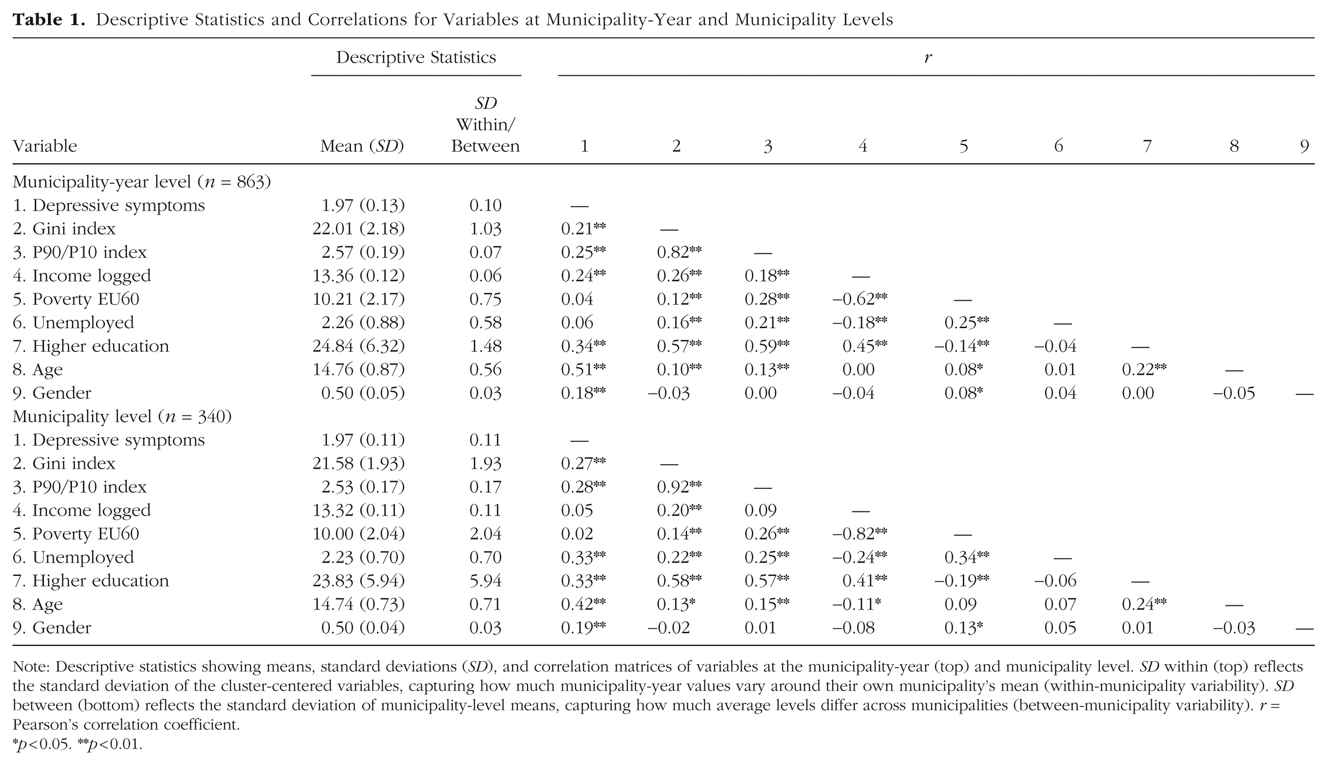
Note: Descriptive statistics showing means, standard deviations (SD), and correlation matrices of variables at the municipality-year (top) and municipality level. SD within (top) reflects the standard deviation of the cluster-centered variables, capturing how much municipality-year values vary around their own municipality’s mean (within-municipality variability). SD between (bottom) reflects the standard deviation of municipality-level means, capturing how much average levels differ across municipalities (between-municipality variability). r = Pearson’s correlation coefficient.

*p < 0.05. **p < 0.01.

Study disclosures

Preregistration: The main hypotheses (Hypothesis 1, Hypothesis 2a, and Hypothesis 2b), methods, and analysis plan were preregistered (https://doi.org/10.17605/OSF.IO/8UW92) on August 6, 2023. The survey data (Ungdata) had already been collected and accessed for use in other research projects before the preregistration. Work on linking Ungdata survey data with registry data from Statistics Norway (SSB) began after preregistration. Thus, the full data set required to test the preregistered hypotheses was not accessed until after preregistration. There were minor and major deviations from the preregistration (see Table S1 in the Supplemental Material). The two major deviations were (a) limiting the time-lagged analyses to 1 to 7 years, rather than 1 to 10 years, because of data constraints identified after gaining access to the full data set and (b) revising the preregistered smallest effect size of interest (SESOI). The preregistered standardized SESOI relied on a heuristic, and it proved uninterpretable once within-municipality variances of the predictors and outcome were known. We therefore redefined the SESOI in unstandardized units using an anchor-based approach tied to diagnostic thresholds for probable depression and self-reported contact with a psychologist to obtain thresholds reflecting realistic and interpretable population-level change. Minor deviations are also documented in Table S1 in the Supplemental Material. Aspects of the work that were not preregistered are described and justified in Table S2 in the Supplemental Material, including descriptive analyses and specification-curve analyses conducted as robustness checks. Materials: All materials are not publicly available, but available through a third party. Detailed documentation of the survey questionnaires used in this study, together with information on access to third-party data and materials, is provided in transparency tables available at https://osf.io/jn4k8/files/peu9s. General information about the Ungdata surveys is available online (https://www.ungdata.no/english/). Data: Because of data-protection regulations and restrictions imposed by the data provider, the raw survey data cannot be shared publicly. The survey data used in this study were obtained from the Ungdata surveys, administered by NOVA at Oslo Metropolitan University. Municipality-level data retrieved from Statistics Norway (SSB) and merged with the survey data are publicly available on the Open Science Framework (OSF; https://osf.io/jn4k8/overview) in the folder “Registry data from Statistics Norway.” To enable reproducibility of the preregistered analyses, we provided synthetic data files that mimic the structure and key relationships of the original data. Results obtained using the synthetic data will approximate, but not reproduce, the numerical values reported in the article. Access to the original Ungdata survey data may be granted upon application to NOVA at Oslo Metropolitan University. See the “Data and Materials Transparency Documentation” linked to above. Analysis scripts: All analysis scripts are publicly available on the OSF at https://osf.io/jn4k8/files/mhy8z. A detailed README file provides step-by-step instructions for restoring the software environment and running the scripts successfully. Using the synthetic data files linked to the R project, the scripts reproduce the full analytical workflow and all main hypothesis tests reported in the manuscript. Note that the results will only approximate, but not reproduce, the numerical values reported in the article. Scripts that load, tidy, and merge the original Ungdata survey data with linked registry data, as well as scripts used exclusively for descriptive analyses based on the full original data, are included for transparency and documentation purposes only and cannot be executed using the synthetic data.

Study Setting, Methodological Overview, and Hypotheses

We analyzed 10 years of nationwide survey data from Ungdata, with more than half a million responses collected at the municipality level in Norway. By linking Ungdata with registry-based measures of municipal income inequality, we examined local within-cluster effects of income inequality following recent methodological recommendations (Sommet & Elliot, 2022; Sommet et al., 2026), using a preregistered protocol of analyses and hypotheses.

We believe that adolescence provides an informative focal point for three reasons: (a) adolescents may be particularly susceptible to mechanisms of status anxiety and competitive motivations; (b) mental disorders tend to debut in adolescence, making it a salient period to observe potential effects of income inequality on mental health; and (c) rising levels of adolescent mental health problems provide a timely context to examine whether changes in income inequality may explain parts of this trend.

Income inequality is often portrayed as affecting all members of society (Wilkinson & Pickett, 2010). However, a recent study found that within-country and within-municipality changes in income inequality were only associated with psychological health among those facing financial scarcity (Sommet et al., 2018). As the authors argue, inequality may threaten psychological health only among those who feel they lack sufficient resources. Studies on adolescents have further suggested that within-country (Elgar et al., 2017) and between-neighborhood (Pabayo et al., 2016) income inequality is associated with psychosomatic and depressive symptoms among adolescent females, but not males. We therefore also test whether the effects of income inequality depend on adolescents’ family financial situation and their gender.

Finally, failures to detect within effects of income inequality may reflect delayed manifestations. If income inequality operates by increasing stress, inducing status anxiety, and reducing the quality of public services, these processes may take time to influence health and well-being (Blakely et al., 2000). Empirical evidence for such lagged effects, however, is mixed. For example, one U.S. study reported that income inequality predicted adult mortality only after a 5-year lag (Zheng, 2012), whereas a more recent study found no lagged effects (1–12 years) on adult happiness and health (Sommet & Elliot, 2022). In adolescent samples, one study found that early-life income inequality predicted more psychosomatic symptoms and lower life satisfaction among adolescent females, but not males (Elgar et al., 2017). Whether these discrepancies reflect differences in samples, measures, or methodological approaches remains unclear.

Building on these considerations, we tested the following preregistered hypotheses:

Hypothesis 1: There is a positive and statistically significant within-municipality effect of income inequality on adolescent depressive symptoms.

Hypothesis 2a: The within-municipality effect of income inequality on adolescent depressive symptoms is positively and statistically significantly stronger among adolescents from families in a poor financial situation than among peers from families in a neutral or good financial situation.

Hypothesis 2b: The within-municipality effect of income inequality on adolescent depressive symptoms is statistically significantly stronger among females than males.

Because a nonsignificant result does not by itself demonstrate that an effect is too small to be of practical relevance, we conducted equivalence tests to assess whether the effect of income inequality can be considered practically negligible (Lakens et al., 2018). Details on these criteria are provided in the Method section. Consistent with our preregistration, we also reexamined these hypotheses using time-lagged variables of income inequality.

Participants and procedure

Data stem from the annual Ungdata surveys, a national data-collection scheme at the municipality level in Norway. Ungdata is the most comprehensive source on adolescent health and well-being in Norway (see https://www.ungdata.no/english/). Ungdata was started in 2010 and has since 2014 been implemented for all junior high and high school students. Since 2010, most Norwegian municipalities have participated, usually every 3 years. Data collection was conducted each spring through an electronic survey administered during school hours, with a teacher or another adult present. Participation was voluntary, and parents of students under 18 years old had the opportunity to withdraw their child from the study. The Ungdata surveys are administered by the Norwegian Social Research (NOVA) at the Oslo Metropolitan University in cooperation with regional drug and alcohol competence centers (KORUS).

The present study used data from the Ungdata surveys from 2010 to 2019 (Frøyland, 2019). The average response rate among participating municipalities has been high, ranging from 75% to 88%. The total sample size pooling all surveys was 628,678 responses nested in 1,064 municipality years and 410 municipalities. Because of anonymity concerns in smaller municipalities (n = 69), age and gender were not assessed. Most of these municipalities had fewer than 5,000 inhabitants, with fewer than 300 individual responses (the majority had fewer than 100). There were also some individual-level missing data on age, gender, financial situation in the family, and on the main outcome measure. The main analytical sample therefore consisted of 863 municipality years (at Level 2), nested in 340 municipalities (at Level 3). Because of individual-level missing data, the number of respondents (at Level 1) varied somewhat across the models testing our main hypotheses (for Hypothesis 1: 563,226; for Hypothesis 2a: 553,380; for Hypothesis 2b: 545,647). Number of municipality-year observations per municipality ranged from 1 to 5, with an average of 2.54 municipality years (SD = 0.91) per municipality (1 = 45, 2 = 118, 3 = 129, 4 = 45, 5 = 3).

Ungdata was merged with official registry data from Statistics Norway (SSB) to obtain municipality-year level information about income inequality and other sociodemographic characteristics. SSB is the national statistical institute of Norway and the main producer of official statistics, responsible for collecting, producing and communicating statistics related to the economy, the population, and the society at multiple levels in Norway (national, regional and local; https://www.ssb.no/en). The data derive from the Ungdata surveys, approved by the Norwegian Centre for Research Data and collected in accordance with national ethical guidelines. Participants provided informed consent, with parental consent provided for students in lower secondary school.

Measures from the Ungdata surveys

Gender and age

Gender was measured by adolescent self-report (female/male). Because of anonymity concerns, age was not explicitly assessed. In Norway, most children start school the year they turn six, attendance in each school grade is organized by birth cohort, and repeating a school grade is generally not practiced. Grade was therefore used as a close proxy for age, with grade 8 corresponding to age 13 and the third year of upper secondary school (equivalent to grade 13 in a continuous grade count) corresponding to age 18.

Symptoms of depression

Depressive symptoms were measured by Kandel and Davies’s six-item Depressive Mood Inventory (DMI). This measure was derived from the Hopkins Symptom Checklist (Derogatis et al., 1974) and assesses depressive symptoms during the preceding week on a 4-point scale from “affected not at all” to “affected extremely.” The six items are summarized to a mean score where a higher score denotes more depressive symptoms (range 1–4). A previous extensive psychometric evaluation of this measure on Ungdata (2010–2019) found that it overall has good psychometric properties, with high internal consistency, evidence of essential unidimensionality, and scalar measurement invariance across survey years when pooling all age groups (Nilsen et al., 2024).

Perceived family financial situation

This item was measured by asking, “Has your family been in a good or poor financial situation over the past two years?” The item was rated on a 5-point rating scale, with response options as follows: 1 = We have been in a good financial situation the whole time, 2 = We have mostly been in a good financial situation, 3 = We have been in neither a good nor a poor financial situation, 4 = We have mostly been in a poor financial situation, and 5 = We have been badly off the whole time. This variable was recoded into a variable with three categories: good financial situation (1 + 2), neutral financial situation (3), and poor financial situation (4 + 5). Subjective assessments of family financial situation have shown robust associations with adolescent health outcomes across studies (Quon & McGrath, 2014). Please note that this measure was labeled “financial scarcity” in the preregistration. For clarity, we relabeled the term to “family financial situation” in the present study, as the item captures the full range from good to poor financial circumstances.

Municipality-year-level measures from Statistics Norway (SSB)

Income inequality. The Gini coefficient was our primary measure of income inequality, which shows the distribution of total income after tax per consumption unit. The Gini lies in the interval between 0 and 1, where 0 indicates that everyone in the population has the same income (i.e., perfect equality), whereas a value of 1 indicates that one single person has all the income (i.e., perfect inequality). As a one-unit increase in the Gini coefficient is not practically possible (it would represent a change in income inequality from 100% equality to 100% inequality), the Gini was multiplied by 100 to yield more sensible and interpretable regression coefficients (the associated change in y given a 0.01 unit = 1 Gini point increase in income inequality).

We also obtained the P90/P10 index to use for robustness analyses. The P90/P10 index is created by sorting the population by income after taxes and dividing the population into 10 equal groups (deciles) on the basis of their income. P90/P10 is the ratio between the income at the 90^th percentile of the population (the income level above which only 10 % earn more) and the income at the 10^th percentile (the income level above which 90% earn more). Thus, whereas the Gini coefficient captures income inequality on the basis of the entire income distribution, the P90/P10 focuses specifically on the gap in income between the top and bottom earners.

Income

Gross median income was calculated on the basis of official registry information from all adult inhabitants per municipality (excluding students).

Poverty rate

Poverty rate was measured by the EU 60 scale. This is a measure of the percentage of the population within each municipality with an equivalized disposable income below 60% of the national median equivalized disposable income (after tax).

Education

Education was measured by the percentage of the population in each municipality that had taken higher education (i.e., at college/university level).

Unemployment

Unemployment was gauged by the percentage registered as unemployed in each municipality. Unemployment in SSB is defined as persons without income-generating work who have attempted to secure such work in the past 4 weeks and who could have taken on work within approximately 2 weeks. Those who were involuntarily fully laid off were considered unemployed after a consecutive duration of 3 months.

Population size

Population size was defined as the number of inhabitants per municipality per year.

Statistical analyses: multilevel linear models

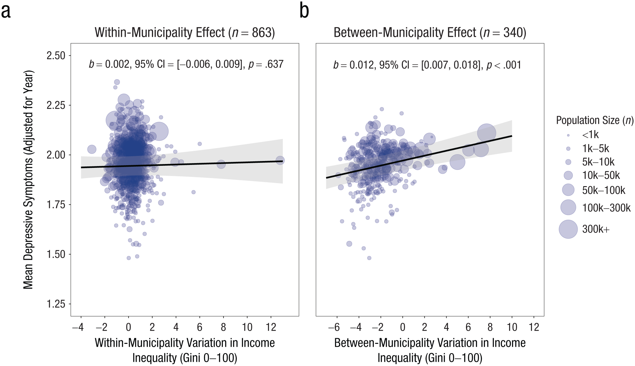
We used multilevel linear models following a preregistered plan of analyses. Ungdata has a three-level structure, with individual respondents nested in municipality years nested in municipalities. To properly model this structure, we included in all analyses random intercepts at the municipality-year level and the municipality level (Schmidt-Catran & Fairbrother, 2016). Models were fitted with restricted maximum likelihood using the lme4 (Bates et al., 2015) and lmerTest (Kuznetsova et al., 2017) packages in R.

Variance decomposition

To estimate the within- and between-municipality effects of income inequality, the variance of the Gini index, along with other municipality-year-level variables, was decomposed into these levels prior to running the analyses. For each municipality, we first computed the mean value of each predictor across all survey years, representing the between-municipality component. We then subtracted this mean from each municipality-year observation to obtain the within-municipality deviation. This can be expressed as

x_{j t} = \bar{x} + ({\bar{x}}_{j} - \bar{x}) + (x_{j t} - {\bar{x}}_{j})

(1)

where $x_{j t}$ is the value of predictor $x$ for municipality $j$ at time $t$ , ${\bar{x}}_{j}$ is the municipality mean, and $\bar{x}$ is the grand mean of all municipalities. The term $({\bar{x}}_{j} - \bar{x})$ quantifies the deviation of a municipality’s mean from the overall (grand) mean (the between-municipality component), whereas $(x_{j t} - {\bar{x}}_{j})$ captures deviations of municipality-year observations from their own municipality mean (the within-municipality component). This decomposition allows both components to be modeled simultaneously, as the within- and between-municipality predictors are orthogonal by construction. It follows the Mundlak (1978) formulation, sometimes referred to as a hybrid model, though this term is debated (see Bell & Jones, 2015). For predictors originally measured at the individual level, these were first aggregated to the municipality-year level before applying the same procedure. Centering municipality means around the grand mean ensures that the model intercept represents the expected outcome when all between-level predictors are held at their average values:

Hypothesis 1 (H1) . To test the first hypothesis, we built a three-level model with random intercepts at the municipality-year level and the municipality level. Following the decomposition above, the general combined equation of this model (Equation 2) may be written as

\begin{array}{l} y_{i j t} = γ_{00} + γ_{20} G i n i_{w i t h i n, j t} + γ_{30} G i n i_{b e t w e e n, j} \\ + γ_{21} W_{j t} + γ_{31} B_{j} + γ_{t} T_{t} + u_{0 j t} + v_{0 j} + e_{i j t} \end{array}

(2)

where $y_{i j t}$ represents depressive symptoms reported by individual $i$ in municipality $j$ at time $t$ ; $γ_{00}$ is the overall intercept. The $γ_{20} G i n i_{w i t h i n},_{j t}$ and $γ_{30} G i n i_{b e t w e e n, j}$ terms capture the within- and between-municipality effects of income inequality, whereas $γ_{21} W_{j t}$ and $γ_{31} B_{j}$ represent a vector of control variables at the within- and between-municipality level. The fixed effect of time (survey-year dummies) is captured by $γ_{t} T_{t}$ . The random intercepts at the municipality-year level and the municipality level are captured by $u_{0 j t}$ and $v_{0 j}$ , whereas $e_{i j t}$ represents the residual error for individual observations. Though our hypotheses concern the within-municipality effect, we also estimate the between-municipality effect, because it serves as an interesting comparison by being the effect that most previous studies have reported findings on. We first tested models also including a random slope of the within-Gini parameter, allowing for the within-effect of income inequality over time to vary between municipalities. However, this yielded convergence issues, most likely due to the little variance captured by our higher-order terms, and was removed from the final models, consistent with our preregistration.

Hypotheses 2a and 2b. To test whether the within-municipality effect was comparatively stronger among those from families in a poor financial situation (H2a) and among adolescent females (H2b), we added cross-level interaction terms between these two Level 1 predictors and income inequality in separate models. These models thus represent a simple extension of Equation 2. For Hypothesis 2a, we used a planned contrast-coding scheme comparing those in a poor financial situation (assigned a weight of + $\frac{2}{3}$ ) with those in a neutral and good financial situation (assigned a weight of – $\frac{1}{3}$ ). We additionally included an orthogonal contrast to ensure that there were no differences between those with a neutral financial situation (assigned a weight of +1) and those with a good financial situation (assigned a weight of −1); we assigned a weight of 0 to those classified as having a poor financial situation.

Considerations regarding control variables

When estimating the effect of income inequality, an important yet difficult task is choosing which variables should be controlled for (confounders) and which should not be controlled for (mediators and colliders). As noted by Connor et al. (2019), this becomes a particular challenge within research on income inequality, where firm empirical evidence about the causal paths between potential predictors, controls, and outcomes is lacking. We have approached this challenge by following a preregistered and prejustified list of controls at the between- and within-municipality levels: gross median income (logged), poverty rate, gender, and age.

Income is associated with income inequality as well as with mental disorders (Kinge et al., 2021). Thus, to ensure that any effect of income inequality is not confounded by within-municipality changes in income, we controlled for municipality-level income. We did not have direct access to individual-level income data, such as parental income. This may be problematic, because nonlinear relationships between individual (or parental) income and health can distort estimates of income inequality on health outcomes. Specifically, small increases in income at the lower end of the income distribution result in disproportionately large improvements in outcomes, whereas additional income at higher levels has diminishing effects. This nonlinearity can confound estimates of income inequality, because low-income individuals may disproportionately influence both income-inequality measures and outcome measures, such as mental health problems (Lynch et al., 2000). To address this limitation, we included municipality-level poverty rate as a control. Poverty rates capture the proportion of individuals at the lower end of the income distribution, where nonlinear effects are most pronounced. Connor et al. (2019) demonstrated that accounting for poverty rates can reduce bias in estimates of income-inequality effects when nonlinear income effects are present. It is worth noting that poverty and inequality are conceptually related, which means that adjusting for poverty may remove variance partly relevant to inequality itself. We nevertheless included poverty because our primary concern was guarding against bias from nonlinear income effects and because the income-inequality hypothesis explicitly posits that inequality should matter even when absolute levels of poverty are adjusted for. As explained below, our robustness checks also examined models with and without poverty included as a covariate. We also performed robustness checks adding perceived family finances as a control, because it may serve as a proxy for parental income.

We added age and gender as control variables at the within and between levels, because there are well-documented age and gender differences in depressive symptoms in adolescence (Nilsen et al., 2024) and because there may be some sampling variability in gender and age distribution both between and within municipalities over time. Finally, time (survey year) was added as a fixed effect, to detrend the estimates (Wang & Maxwell, 2015). Both income inequality and depressive symptoms have increased in recent decades, so detrending mitigates the possibility that these parallel trends may confound the within-municipality effect of income inequality.

Education and unemployment were not added as controls in our main preregistered models, because their status as potential mediators have been argued by some (i.e., that education and unemployment lie on the causal pathway between income inequality and health outcomes; Pickett & Wilkinson, 2015). However, we included them in our study to assess the sensitivity of our results to alternative covariate specification.

Equivalence testing

We conducted equivalence tests to evaluate whether the within-municipality effects of income inequality were too small to be of practical importance. This required defining an SESOI. In our preregistration, we used a standardized coefficient of ±0.05 to denote a very small, and likely inconsequential, effect. However, this threshold later proved implausibly small (≈ 0.0065 DMI units per 1-point Gini change) and lacked substantive interpretability, something that could not have been known at preregistration because the within-cluster standard deviations of both predictors and outcomes were not yet available.

Given these limitations of the preregistered heuristic, we redefined the SESOI and thus the equivalence range on the raw scale using an anchor-based approach (Anvari & Lakens, 2021; Lakens et al., 2018). Details are provided in the Supplemental Material (Section 2). In brief, we drew on two complementary anchors: (a) diagnostic thresholds for probable depression and (b) self-reported contact with a psychologist. Organisation for Economic Co-operation and Development (OECD) reports often characterize a 2-point change in the Gini coefficient as a notable shift in inequality, whereas movements of 5 points appear large and historically rare (OECD, 2015). SESOIs were therefore anchored around the expected population-level consequences of a 2-point change in the Gini coefficient, representing roughly a 9% change relative to the mean municipal Gini of 21.6 in our data.

Both anchors suggested that a ±0.015-unit change on the DMI per 1-point change in the Gini coefficient represents a conservative threshold for practical relevance, corresponding to a percentage-point difference of roughly 1.3 in the prevalence of probable depression and a percentage-point difference of 0.2 in psychologist contact for a 2-point Gini change. For interaction effects, we applied a narrower range (±0.0125 DMI). On the basis of our anchor translations, such an interaction would correspond to a divergence between groups—for instance, between females and males—of approximately 1.1 percentage points in the prevalence of probable depression and 0.12 percentage points in psychologist contact for a 2-point Gini change (see Tables S3–S4 in the Supplemental Material). We treat these magnitudes as very small and conservative thresholds for substantive interpretation while acknowledging that defining practically meaningful effects inevitably involves judgment.

Deviating from our preregistered SESOI and redefining the equivalence bounds is not ideal and results in a less stringent assessment of equivalence. In this case, however, the preregistered standardized bound could not be meaningfully interpreted once the within-cluster variances were known, and updating the SESOI was necessary to obtain thresholds that reflect realistic and interpretable population-level change. Defining what constitutes a practically meaningful effect of income inequality is inherently challenging, and others may prefer stricter or more lenient thresholds. To facilitate such evaluation, we show in our Supplemental Materials predicted changes in both anchors across a range of alternative SESOIs, allowing readers to judge practical significance under stricter or more lenient thresholds.

Equivalence was assessed using 90% confidence intervals (CIs): If the entire 90% CI fell within the SESOI bounds, we interpreted the effect as too small to be of practical relevance (i.e., statistically equivalent to a negligible effect), whereas any partial overlap was treated as inconclusive (Lakens et al., 2018). Conventional null-hypothesis tests based on 95% CIs were used separately to evaluate whether effects differed from zero. We present the equivalence estimates and their CIs visually in the figures here for ease of interpretation.

Power

To assess that the revised SESOIs were empirically realistic, we conducted a simulation-based design-analysis on the fitted multilevel models (see Supplementary Section 3 for all details). The analysis evaluates the long-run operating characteristics of our models given their actual structure and variance components (Gelman & Carlin, 2014). This approach is useful for complex multilevel models in which power depends not only on sample size but also on variance components and clustering structures that are difficult to specify in advance (Arend & Schäfer, 2019). Using the observed clustering, sample imbalance, and variance parameters, we generated 1,000 data sets (b = 0) and reestimated each of our focal models to determine the probability that the 90% CI would fall fully within a range of alternative SESOI bounds, as an assessment of equivalence power (Lakens, 2017). This procedure ensured that our chosen SESOIs were not only substantively anchored but also statistically testable given the study’s design. Results showed near-complete power to detect equivalence (~1.00) for the main within- and gender-related effects, good power for the poor group (~0.83), but somewhat lower power for the Poor × Gini interaction (~0.68; see Table S5 in the Supplemental Material). We also assessed detection power (i.e., the power to detect a significant effect) across a subset of potential SESOIs, following the same approach, which naturally gave slightly higher power per estimate as it requires less to detect an effect than to conclude equivalence (Table S6).

Robustness and sensitivity analyses

Specification-curve analyses

We performed specification-curve analyses to evaluate how sensitive the results from our preregistered models were to alternative model specifications. Specification-curve analyses involve selecting theoretically defensible models that represent plausible variations in the analysis (Simonsohn et al., 2020). For the within-municipality effect, we considered all available municipality-year-level variables as potentially defendable, including median income, poverty rate, unemployment rate, education levels, and age and gender distribution. For Hypothesis 1 and Hypothesis 2b, we also included family financial situation as a Level 1 covariate. The preregistered models already adjusted for area-level poverty rate to help reduce potential bias from nonlinear individual income effects (Connor et al., 2019), but we also recognize that perceived family financial situation serves as a complementary individual-level proxy, and we thus included it as an additional robustness check. This resulted in 128 multilevel models for Hypothesis 1 and Hypothesis 2b and 64 models for Hypothesis 2a, each with a unique combination of these covariates, tested against our focal hypotheses. In all these models, for consistency we retained the same Level 3 (municipality-level) covariates as in our original analyses (note that these are uncorrelated with the Level 2 variables). We also kept time (survey year) as a fixed effect in all models, because the importance of accounting for the possibility of simultaneous trends (i.e., that income inequality and adolescent depressive symptoms have increased over time) is established and uncontroversial.

For comparison, we also conducted specification-curve analyses for the between-municipality effects using the equivalent between-municipality covariates. We present the results visually as specification-curve plots showing how each combination of covariates affected the estimates of the within- and between-effect estimate of income inequality.

Lagged effects

We reexamined Hypotheses 1 and 2 using time lags of the within-municipality effect. The time lags were created by substituting the municipality-level Gini index measured at time t0 (the current year) with the municipality-level Gini measured at t−1 (1 year earlier), t−2 (2 years earlier), and up to t−7 (7 years earlier; for a similar approach, see Sommet & Elliot, 2022). Because the registry data on income inequality (and other measures) from SSB only goes back to 2005, we limited our analysis to a total of seven time lags, as going further back quickly diminished the number of municipality years available for analysis. Thus, the lagged within-municipality effect of income inequality in these analyses represents the deviation of income inequality in a municipality at t−x (where x denotes the number of years lagged) from the average municipality income inequality in the period from 2005 to 2019.

With seven lags, we conducted a total of 21 new multilevel analyses (7 lags × 3 hypotheses). For each of these models, we included the respective time-lagged within-municipality variable (e.g., t−1) in addition to the yearly (t0) within-municipality effect. Thus, the estimates of each time lag represent the extent to which income inequality as measured at t−x was associated with depressive symptoms after controlling for the contemporaneous within-municipality changes in income inequality. We also conducted a joint model that included all time-lagged variables simultaneously as predictors, in order to control for a series of previous and contemporaneous income inequalities (Zheng, 2012). As we noted in our preregistration, we consider these analyses exploratory because we had no strong a priori expectations of when an eventual time lag should produce an effect on adolescent depressive symptoms.

Moderation by population size

It has been argued that the effect of income inequality on health should be more pronounced in larger compared with smaller areas (Pickett & Wilkinson, 2015). Although this argument originally pointed to differences between areas such as countries, states, and neighborhoods, we exploit the fact that the population size of Norwegian municipalities differs widely (from fewer than < 1,000 inhabitants to more than 500,000), and we examine the degree to which the within-municipality effect of income inequality on depressive symptoms depends on population size. We here used, as our measure of municipality population size, the grand-mean-centered municipality mean of population size of each municipality calculated from the years 2010 to 2019. In addition, we reran our focal model as specified in Equation 2, with the addition of a cross-level interaction term between within-municipality income inequality and municipality population size and an interaction term of the between-municipality income-inequality term and municipality population size.

P90/P10 index

Finally, all main analyses were rerun substituting our preferred measure of income inequality with the P90/P10 index, to assess whether results converged across another commonly used indicator of income dispersion. Whereas the Gini coefficient captures inequality across the entire income distribution, the P90/P10 index focuses specifically on the gap between the highest and lowest earners and is therefore more sensitive to changes at the extreme ends of the distribution. Because a one-unit change in the raw P90/P10 ratio would imply an unrealistically large widening of the income gap, far beyond any plausible within-municipality fluctuation (the mean municipal P90/P10 ratio was about 2.53), we rescaled the within-municipality component so that a 1-unit change corresponded to a 0.05 increase in the ratio, which in our data is approximately 1 within-municipality SD. According to official 2024 income percentile statistics from Statistics Norway (2025), a 0.05 change in P90/P10 corresponds to a widening of the annual income gap of approximately $2,200 USD (about 22,170 NOK). Such a widening can materialize through different underlying patterns; for example, if the bottom 10% earn $2,200 (US) less, if the top 10% earn $2,200 more, or through some combination of both.

Because the P90/P10 analyses were conducted to evaluate whether conclusions converged across an alternative inequality metric, we did not define a distinct SESOI for this measure. The Gini-anchored SESOI cannot be directly transferred to P90/P10, as the two indices quantify different aspects of the income distribution and cannot be placed on a common scale through any direct transformation. However, the anchors we developed for the outcome (that is, expected changes in depressive symptoms and psychologist contact) still provide a useful point of reference for gauging the substantive size of effects obtained with P90/P10. We therefore interpreted P90/P10 coefficients descriptively in light of these outcome-based anchors, while relying on the Gini coefficient as the primary inequality indicator for formal equivalence testing.

Results

Descriptive characteristics of the variables and the correlations at both the municipality-year level and the municipality level are presented in Table 1, including the variability of each measure within and between municipalities (SD-within and SD-between). Note that the correlations reflect cross-sectional associations at their respective aggregation levels, not the decomposed within- and between-municipality effects estimated in the multilevel models.

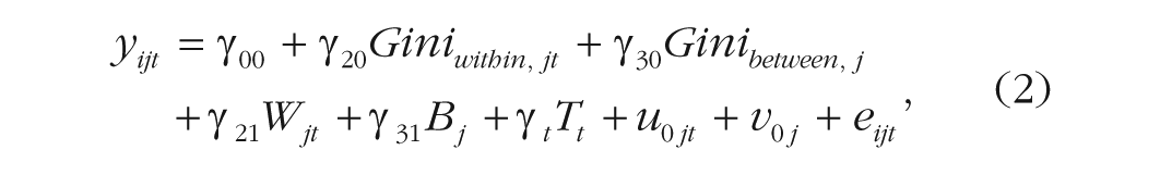
The crude associations of the within- and between-municipality effects, only adjusted for time fixed effects, are visualized in Figure 1. At the within level (Fig. 1a), no clear association between within-municipality income inequality (as measured by the Gini index) and adolescent depressive symptoms was observed. At the between level (Fig. 1b), a significant and positive association was observed in which municipalities with higher income inequality tended to have adolescents with higher levels of depressive symptoms.

Fig. 1.

Adjusted scatterplot showing the relationship between variation in income inequality and depressive symptoms, controlling for year fixed effects. The observed data points have been adjusted for the effect of year by subtracting the estimated year effects from a simplified multilevel model on data aggregated to the municipality-year level, including random intercepts at the municipality level. Within-municipality variation is shown in (a) and between-municipality variation is shown in (b). The within-municipality variation represents the municipality-year deviation from the municipality mean, whereas the between-municipality variation represents the municipality mean deviation from the grand mean of all municipalities. The regression lines are based on predicted values from the multilevel model. Shaded regions are model-based 95% confidence intervals (CIs). The points are sized according to the mean population size of municipalities in the years 2010 to 2019.

The within-municipality effects of income inequality

Figure 2 presents the substantive results from our preregistered models addressing the main hypotheses. Full model results are shown in Table S7 in the Supplemental Material (the numerical estimates underlying the figure are provided in Table S8). Overall, no significant within-municipality effect of income inequality on adolescent depressive symptoms was detected (H1: b = 0.002, 90% CI = [−0.002, 0.006], p = .473), with 90% CIs falling well within the equivalence range (±0.015). Thus, the overall effect of income inequality was not significantly different from zero and was judged as too small to be practically meaningful.

Fig. 2.

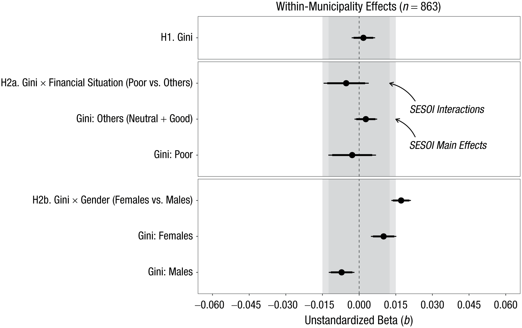
Unstandardized beta coefficients (b) for the within-municipality effects of income inequality on adolescent depressive symptoms. The light-gray shaded area marks the equivalence range for the main effects (±0.015). The darker inner band (±0.0125) denotes the equivalence range for the interaction effects. Black points indicate model-based point estimates, with thick horizontal lines showing 90% confidence intervals and thinner lines showing 95% confidence intervals. The vertical dashed line marks the classical null hypothesis (b = 0). H1 = Hypothesis 1; H2a = Hypothesis 2a; H2b = Hypothesis 2b; SESOI = smallest effect size of interest.

Similarly, no significant cross-level interaction between within-municipality income inequality and poor financial situation was observed (Hypothesis 2a; b = −0.005, 90% CI = [−0.013, 0.002], p = .260). However, the lower 90% CI crossed the lower equivalence bound for interactions (−0.0125), meaning that the result of the equivalence test was inconclusive. Still, main effects for both adolescents from poor and nonpoor families were small, nonsignificant, and within the equivalence range. Taken together, these results suggest that although the presence of a practically meaningful interaction cannot be rejected, the main effects for both groups were too small to be considered meaningful.

For gender (Hypothesis 2b), a significant cross-level interaction was detected, suggesting that the effect of within-municipality income inequality was significantly stronger among adolescent females than males (b = 0.017, 90% CI = [0.014, 0.020], p < .001). This interaction was deemed practically meaningful, because the 90% CI lay entirely outside the equivalence range. Translated into predicted prevalence, the interaction corresponds to a difference of roughly 1.1 percentage points in probable depression between females and males and about 0.12 to 0.16 percentage points in the prevalence of contact with a psychologist for a +2 Gini increase.

In contrast, the main within-municipality effects for males (b = −0.007, 90% CI = [−0.011, −0.003]) and females (b = 0.010, 90% CI = [0.006, 0.014]) were both statistically significant but fell entirely within the predefined equivalence bounds (±0.015), indicating effects that are statistically detectable but too small to meet our criterion for practical relevance. These coefficients translate to a higher prevalence of probable depression for females (≈ 0.8 percentage points) and a lower prevalence for males (≈ 0.6 percentage points) with a +2 Gini increase; changes in psychologist contact were ≈ 0.2 and ≈ −0.1 percentage points, respectively.

The between-municipality effects of income inequality

At the between-municipality level, a positive association between income inequality and depressive symptoms was observed overall (b = 0.012, 95% CI = [0.006, 0.017]), indicating that municipalities with higher income inequality also tended to report higher average levels of adolescent depressive symptoms. No significant cross-level interaction between income inequality and family financial situation was detected. For gender, the associated effect of income inequality was positive for both males (b = 0.014, 95% CI = [0.009, 0.019]) and females (b = 0.009, 95% CI = [0.005, 0.014]), and the gender difference was statistically significant (b = −0.005, 95% CI = [−0.006, −0.004]), suggesting a somewhat stronger association among males (see Table S7).

Robustness and sensitivity analyses

The results from the specification-curve analyses for each hypothesis are shown in Figure 3. For hypotheses concerning the within effect of income inequality, the estimates from the preregistered model (shown in red) were highly similar to the estimates obtained from all other model specifications tested, suggesting that the choice of including (or excluding) a given within-municipality covariate had no meaningful impact on our main results.

Fig. 3.

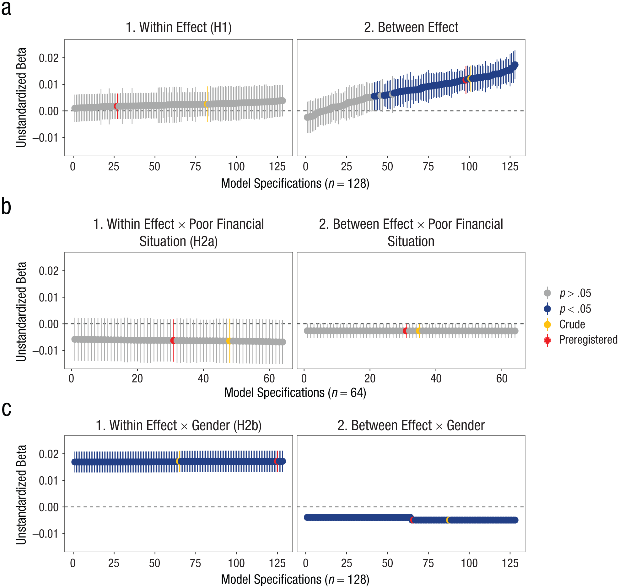
Results from specification-curve analyses testing a total of 128 different combinations of covariates when assessing the within-municipality and between-municipality effects of income inequality for Hypothesis 1 (H1) and Hypothesis 2b (H2b), and 64 different covariate specifications for Hypothesis 2a (H2a). The graphs to the left (a to c, denoted “1”) show the within-municipality effects, whereas the graphs to the right (a to c, denoted “2”) show the between-municipality effects. The gray and blue colors signify whether the estimates were p > .05 or p < .05, respectively; the yellow dots signify the crude estimates (without any controls except year fixed effects); and the red dots signify the estimates from the preregistered models.

At the between level, the main between effect of municipality income inequality showed more variability, with 84 model specifications yielding statistically significant associations and 44 yielding nonsignificant associations. The common denominator in the latter models was the inclusion of between-municipality educational levels as a covariate. In other words, if we held the proportion of the adult population with higher education constant between municipalities, income inequality had no significant association with adolescent depressive symptoms between municipalities.

Lagged effects of income inequality

Across all time lags, here labeled t−1 through t−7, no practically meaningful main effects of within-municipality income inequality on adolescent depressive symptoms were detected (Hypothesis 1; Fig. 4). For interactions with family financial situation (Hypothesis 2a; Fig. 5a), one model indicated a statistically significant and practically nonequivalent difference between adolescents from poor versus nonpoor families: At lag t−1, the poor-versus-others interaction was negative and exceeded the equivalence bounds (b = −0.010, 90% CI = [−0.0185, −0.0017])—that is, opposite to the hypothesized direction. The corresponding main effect for adolescents from poor families at t−1 (b = −0.0091, 90% CI = [−0.0185, 0.0003]) was not statistically significant but crossed the lower equivalence bound (−0.015), rendering the result inconclusive with respect to practical equivalence. For all other lags, the main effects for adolescents from poor and nonpoor families were neither statistically significant nor practically meaningful (see Tables S9–S11 in the Supplemental Material for numerical estimates).

Fig. 4.

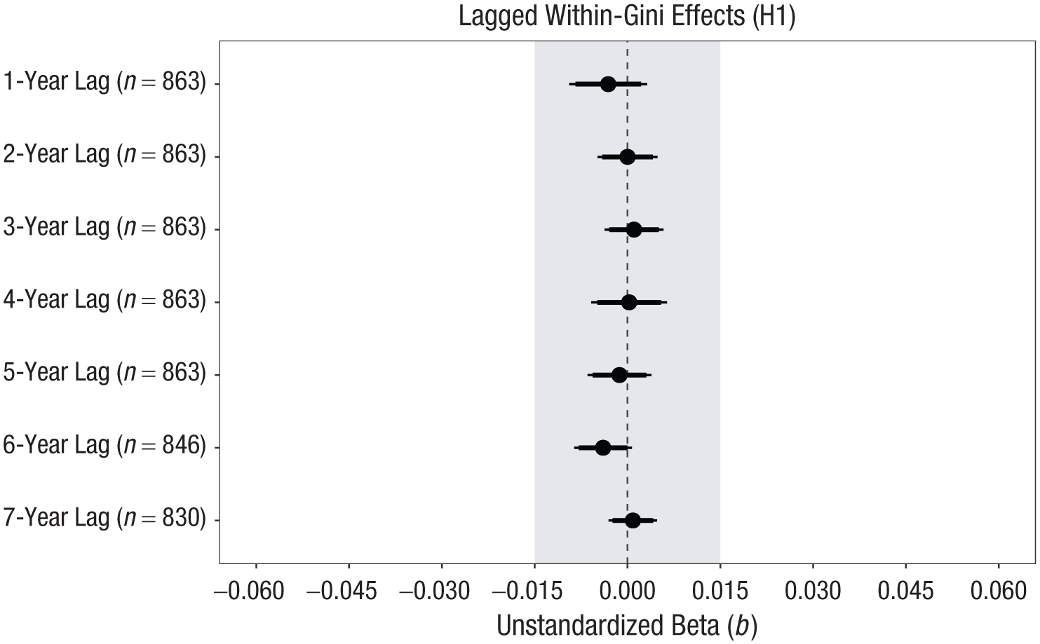
Unstandardized beta coefficients (b) for the effects of time-lagged within-municipality income inequality on adolescent depressive symptoms. The shaded gray area illustrates the equivalence range, defined from −0.015 to 0.015. Black points indicate the model-based estimates of b. Thick horizontal lines show the 90% confidence intervals, and thinner horizontal lines represent the 95% confidence intervals. The vertical dashed line marks the classical null hypothesis (b = 0). H1 = Hypothesis 1.

Fig. 5.

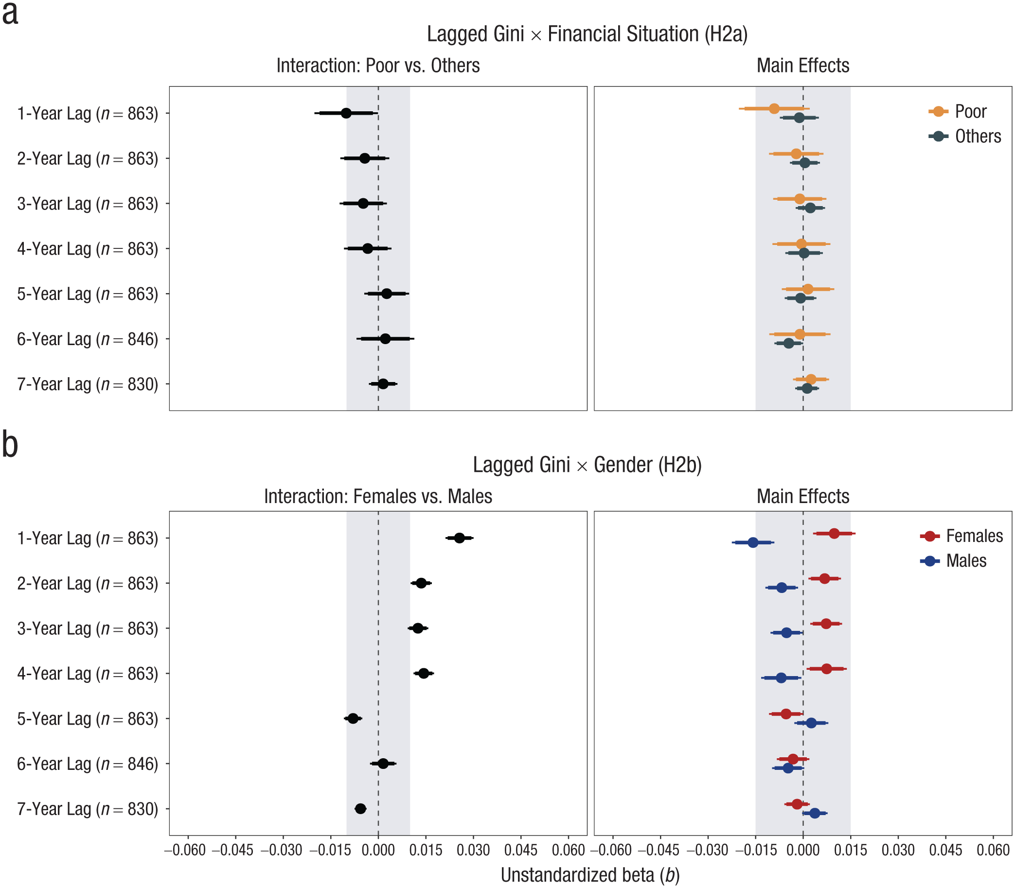
Unstandardized beta coefficients (b) for the effects of time lagged within-municipality Gini index on adolescent depressive symptoms across Hypotheses 2a and 2b. In (a) we show the effect of the time lagged within-municipality effects in interaction with perceived family financial situation, and in (b) we show the effect of the time-lagged within-municipality effects in interaction with gender. The shaded gray area illustrates the equivalence range, defined as ±0.0125 for interaction terms and ±0.015 for main effects. Points indicate the model-based estimates of b. Thick horizontal lines show the 90% confidence intervals, and thinner horizontal lines represent the 95% confidence intervals. The dashed vertical line marks the classical null hypothesis (b = 0). H2a = Hypothesis 2a; H2b = Hypothesis 2b.

For gender (Hypothesis 2b; Fig. 5b), the interaction was fully outside the equivalence range at t−1, t−2, and t−4, suggesting that within-municipality changes in income inequality were associated with depressive symptoms in a meaningfully different way among females than males. Looking at the main effects for these time lags, within-municipality changes in income inequality were positively associated with depressive symptoms in females and negatively associated in males. However, only at t−1 did the main effects cross the equivalence range, indicating that the possibility of a practically meaningful main effect for males and females could not be rejected.

Joint models including all time lags simultaneously (see Tables S12–S14) did not change the overall interpretation: almost all estimates lay within their respective equivalence bounds, and conclusions matched those from the single-lag analyses.

Moderation by municipality population size

As shown in Table S15, the main within-municipality effect of income inequality did not significantly vary by municipality population size.

The P90/P10 index as an alternative metric of income inequality

The robustness analyses using the P90/P10 ratio reproduced the same overall pattern as the Gini index (see Figures S12–S14 and Tables S16–S18). The only consistent signal was again the gender interaction: females showed a stronger positive association than males across several lags, and these interactions were statistically significant for the main within effect and for the early time lags (Table S18). As in the Gini models, the underlying main effects for females and males pointed in opposite directions (positive for females, negative for males), but were small in magnitude.

A 1-unit increase in P90/P10 (that is, a 0.05 increase in the ratio, an increase of about 1 within SD, and roughly a $2,200 widening of the income gap) produced a main within-municipality effect that was not statistically significant and close to zero (b = −0.001, 95% CI = [−0.006, 0.004]). For the main gender effects, approximately two within-SD changes in the P90/P10 (a widening income gap around $4,400) were needed for estimates to approach the meaningful cut defined by our SESOI of a 0.030-point change in the DMI, corresponding to about a 1.2% increase in probable major depressive episode.

In sum, the results using the P90/P10 yielded the same overall pattern as the Gini. Although the gender interaction indicated meaningfully different associations for females and males, the underlying main effects for both groups were small. A large shift in the within-municipality income distribution between the P90 and the P10 would be required to produce changes in adolescent depressive symptoms that may be viewed as practically meaningful.

Discussion

Income inequality has been positioned as one of the defining challenges of our era, due in part to its assumed impact on psychological health (Gobel & Carvacho, 2024). However, in this large repeated-cross-sectional study, we found no evidence that changes in income inequality were meaningfully associated with adolescent depressive symptoms overall. This result mirrors previous studies reporting nonsignificant within effects on mental health, well-being, and mortality (Hiilamo, 2014; Jørgensen & Hovde Lyngstad, 2024; Sommet & Elliot, 2022). In particular, this finding replicates those of Sommet and Elliot (2022), where within-county and within-state effects of income inequality on happiness and health in the United States were deemed too small to be considered practically meaningful.

Similarly, we found no clear evidence that the within effects of income inequality were moderated by financial situation, contrasting with a prior study reporting associations only among individuals facing financial scarcity (Sommet et al., 2018). Several explanations are possible. Measurement differences may matter, because our indicator captures a broader assessment of perceived family finances, whereas the earlier study focused more narrowly on scarcity. In addition, the Norwegian welfare context, with universal schooling and health care and policy efforts to reduce social inequalities in health (Fosse, 2022), may shape both the experience of financial strain and how it interacts with broader income inequality. Another explanation concerns statistical power. Sommet et al. (2018) analyzed more than 15,000 municipality years, which provided much greater sensitivity to detect very small cross-level interactions. In our simulation-based design analysis, power to conclude equivalence for the Poor-versus-Others × Gini interaction was modest, about 0.68 at ±0.0125, which means we had more limited ability to rule out very small interaction effects. Hence, we do not view our finding as definitive evidence that no interaction exists, but rather as indicating that any such effect, if present, is likely to be small and of limited substantive importance in this context.

We found some evidence that the association between changes in income inequality and adolescent depressive symptoms differed by gender, in line with our preregistered hypothesis (Hypothesis 2b) and aligning with Elgar et al. (2017). The gender interaction was statistically significant and fell outside the equivalence bounds in the main model and across several time-lagged specifications (t−1 to t−4), indicating meaningfully different associations for females and males. However, the corresponding main effects within each gender were generally small, and only one model specification (at t−1) produced main effects for males and females that fell outside the equivalence bounds. At that lag, the associations moved in opposite directions, positive for females and negative for males. If taken as real and substantively meaningful effects, this pattern would require a convincing theoretical explanation, as it implies that rising inequality benefits boys’ mental health while worsening girls’. Given that this pattern was isolated, and that the remaining main effects were consistently small and too small to be considered practically meaningful, we viewed the evidence for meaningful gender-specific effects as weak.

We acknowledge that demarcating a practically meaningful effect of income inequality is challenging. Others may disagree with our choice, because small effects can be meaningful when accumulated over time (Funder & Ozer, 2019). However, we do not believe that the gender differences found provide strong support for the notion of income inequality as a forceful determinant of psychological health within the context studied here, even if restricted to females. Moreover, though the within-cluster level of analysis offers benefits in terms of statistical control by removing time-invariant confounding, other unobserved time-varying factors likely exist that to some extent confound our estimates. If so, such small effects may quickly attenuate toward zero.

To put the observed effects in perspective within the context of rising adolescent depressive symptoms, our results indicate that changes in income inequality are unlikely to have made a meaningful contribution. The observed increase among girls from 2010 to 2019 in Ungdata corresponds to about a 0.24 unit rise on the DMI scale. In our models, a 1-point within-municipality increase in the Gini index was associated with a 0.01-unit increase in DMI among girls. Thus, for income inequality alone to account for this observed rise, the Gini index would have had to increase by more than 20 points, effectively doubling Norway’s current level of inequality and moving it from among the most equal countries to levels of far more unequal countries. This calculation already rests on the generous assumptions that the estimate reflects a true causal effect, that no unmeasured time-varying confounders exist, and that the estimated effect scales linearly across a wider range of inequality than what was observed—conditions that are unlikely to hold.

Pickett and Wilkinson (2015) argue that studies finding no association between income inequality and health often suffer from overcontrol bias, inadequate time frames, or inappropriate cluster sizes. Regarding overcontrol bias, the specification-curve analyses showed our findings were robust to alternative covariate specifications, even when no controls except for time were included. Thus, overcontrol bias cannot explain our results. Our conclusion also held after accounting for up to 7-year time lags. Although some conditions, such as chronic illness or mortality, may need more time to show effects, self-rated health is likely responsive to more immediate changes in social conditions (Zheng, 2012). Finally, as autonomous entities with their own political governance, economies, and public services, we believe that municipalities represent a meaningful level to detect a contextual effect of income inequality, should it exist.

Although our results do not support the notion that changes in income inequality have produced more depressive symptoms among adolescents in Norway, this does not imply that income inequality is desirable or acceptable. There may be other good moral and political reasons to promote greater equality. Income inequality may also be associated with other psychological processes than those studied here. For example, research indicates that income inequality could lead to more competitiveness (Sommet et al., 2023) and risk taking (Payne et al., 2017) and bullying (Elgar et al., 2019).

Strengths and Limitations

Strengths of this study include 10 years of repeated cross-sectional survey data with a high response rate, comprising over half a million adolescent responses from 863 municipality years merged with objective registry data on municipality characteristics, providing high power to detect small within-municipality effects. Another strength was the simultaneous estimation of within and between estimates, following a preregistered plan of analyses and model specifications. Additionally, specification-curve analyses provided a transparent overview of how covariate selection affected our results. Moreover, whereas some previous studies have used single-item measures as indicators of mental health (Sommet et al., 2018; Sommet & Elliot, 2022), we used a multi-item instrument of depressive symptoms that has been found to have good psychometric properties in this sample.

Several limitations should be noted. First, although multilevel analyses are well equipped to handle unbalanced panel designs, more reliable within estimates could have been obtained if more municipality-year observations per municipality existed. Relatedly, although we accounted for the main dependence structure of the data, we cannot rule out the possibility that a subset of respondents participated more than once. We examined this in Section 7 in the Supplemental Material and found that repeated participation was modest. Although such dependence could bias standard errors or test statistics, it is unlikely to affect the substantive conclusions given the size and structure of the data set.

Second, it may be that a threshold of change in income inequality must be reached before its impact on mental health becomes evident. Given that the changes were overall modest, it is possible that this threshold was not met. However, this does not seem to be a unique feature of our study context, as similar within-county Gini variability has also been reported in the United States (Sommet & Elliot, 2022). Consequently, our results speak to the effects of the realistic policy-relevant shifts in inequality that occur in Norwegian municipalities, rather than to hypothetical large-scale changes that are rarely observed in this context.

A further limitation concerns the SESOI. The preregistered standardized SESOI proved difficult to interpret once the within-municipality variance was known, and we therefore redefined it in unstandardized units. This deviation makes the equivalence tests less stringent than originally planned, but we viewed the respecified SESOI as necessary, because it provides a clearer and more contextually grounded benchmark.

Conclusions

At a time of rising adolescent depressive symptoms, within-municipality changes in income inequality do not seem to meaningfully predict changes in adolescent depressive symptoms in Norway. If there is a positive association, our findings suggest that it may be limited to females. However, the small effects detected make us question whether they are practically meaningful in understanding changes in recent population mental health trends. Though our results may be bound to the conditions studied here, we believe they add value to a research field dominated by low-powered cross-sectional designs. Insofar as income inequality continues to be framed as a universal contextual effect affecting the mental health of all, our results suggest that this view should be tempered, at least when considering adolescent depressive symptoms in Norway.

Supplemental Material

sj-pdf-1-pss-10.1177_09567976261432207 – Supplemental material for Does Income Inequality Predict Adolescent Depressive Symptoms?

Supplemental material, sj-pdf-1-pss-10.1177_09567976261432207 for Does Income Inequality Predict Adolescent Depressive Symptoms? by Sondre Aasen Nilsen, Kyrre Breivik, Kjell Morten Stormark and Tormod Bøe in Psychological Science

Footnotes

Acknowledgements

We would like to thank all the adolescents who participated in Ungdata, making this study possible. We also extend our gratitude to NOVA and the regional competence centers for substance use (KORUS) for their continuous efforts in conducting and maintaining the Ungdata surveys. We further thank Morten Nordmo for independently verifying the computational reproducibility of the analyses and for confirming that the code works even when he runs it.

Transparency

Action Editor: Amy Orben

Editor: Simine Vazire

Author Contributions

Sondre Aasen Nilsen: Conceptualization; Data curation; Formal analysis; Methodology; Project administration; Software; Visualization; Writing – original draft; Writing – review & editing.

Kyrre Breivik: Conceptualization; Methodology; Writing – review & editing.

Kjell Morten Stormark: Conceptualization; Data curation; Project administration; Writing – review & editing.

Tormod Bøe: Conceptualization; Investigation; Methodology; Writing – review & editing.

ORCID iDs

Sondre Aasen Nilsen

Kyrre Breivik

Kjell Morten Stormark

Tormod Bøe

Supplemental Material

Additional supporting information can be found at

References

Anvari

Lakens

(2021). Using anchor-based methods to determine the smallest effect size of interest. Journal of Experimental Social Psychology, 96, 104159. https://doi.org/https://doi.org/10.1016/j.jesp.2021.104159

Arend

M. G.

Schäfer

(2019). Statistical power in two-level models: A tutorial based on Monte Carlo simulation. Psychological Methods, 24(1), 1–19. https://doi.org/10.1037/met0000195

Bates

Mächler

Bolker

Walker

(2015). Fitting linear mixed-effects models using lme4. Journal of Statistical Software, 67(1), 1–48. https://doi.org/10.18637/jss.v067.i01

Bell

Jones

(2015). Explaining fixed effects: Random effects modeling of time-series cross-sectional and panel data. Political Science Research and Methods, 3(1), 133–153. https://doi.org/10.1017/psrm.2014.7

Blakely

T. A.

Kennedy

B. P.

Glass

Kawachi

(2000). What is the lag time between income inequality and health status? Journal of Epidemiology & Community Health, 54(4), 318–319. https://doi.org/10.1136/jech.54.4.318

Brunborg

G. S.

Nilsen

S. A.

Skogen

J. C.

Bang

(2025). Possible explanations for the upward trend in mental distress among adolescents in Norway from 2011 to 2024. Social Science & Medicine, 384, Article 118528. https://doi.org/10.1016/j.socscimed.2025.118528

Cheung

(2018). Income redistribution predicts greater life satisfaction across individual, national, and cultural characteristics. Journal of Personality and Social Psychology, 115(5), 867–882. https://doi.org/10.1037/pspp0000164

Connor

Sarafidis

Zyphur

M. J.

Keltner

Chen

(2019). Income inequality and White-on-Black racial bias in the United States: Evidence from Project Implicit and Google Trends. Psychological Science, 30(2), 205–222. https://doi.org/10.1177/0956797618815441

Derogatis

L. R.

Lipman

R. S.

Rickels

Uhlenhuth

E. H.

Covi

(1974). The Hopkins Symptom Checklist (HSCL): A self-report symptom inventory. Behavioral Science, 19(1), 1–15. https://doi.org/10.1002/bs.3830190102

10.

Chi

King

R. B.

(2019). Economic inequality is associated with long-term harm on adolescent well-being in China. Child Development, 90(4), 1016–1026. https://doi.org/10.1111/cdev.13253

11.

Elgar

F. J.

Gariepy

Dirks

Walsh

S. D.

Molcho

Cosma

Malinowska-Cieslik

Donnelly

P. D.

Craig

(2019). Association of early-life exposure to income inequality with bullying in adolescence in 40 countries. JAMA Pediatrics, 173(7), e191181. https://doi.org/10.1001/jamapediatrics.2019.1181

12.

Elgar

F. J.

Gariépy

Torsheim

Currie

(2017). Early-life income inequality and adolescent health and well-being. Social Science & Medicine, 174, 197–208. https://doi.org/10.1016/j.socscimed.2016.10.014

13.

Elgar

F. J.

Pförtner

T.-K.

Rothwell

(2024). Socioeconomic differences and global trends in youth wellbeing and emotional distress in 165 countries and territories. Health & Place, 89, Article 103322. https://doi.org/10.1016/j.healthplace.2024.103322

14.

Fosse

(2022). Norwegian policies to reduce social inequalities in health: Developments from 1987 to 2021. Scandinavian Journal of Public Health, 50(7), 882–886. https://doi.org/10.1177/14034948221129685

15.

Frøyland

L. R.

(2019, June 19). Ungdata, 2010-2019. Sikt - Kunnskapssektorens tjenesteleverandør. https://doi.org/10.18712/NSD-NSD2711-V1

16.

Funder

D. C.

Ozer

D. J.

(2019). Evaluating effect size in psychological research: Sense and nonsense. Advances in Methods and Practices in Psychological Science, 2(2), 156–168. https://doi.org/10.1177/2515245919847202

17.

Gaspar

R. S.

Rossi

Hone

Dornelles

A. Z.

(2021). Income inequality and non-communicable disease mortality and morbidity in Brazil States: A longitudinal analysis 2002-2017. The Lancet Regional Health–Americas, 2, Article 100042. https://doi.org/10.1016/j.lana.2021.100042

18.

Gelman

Carlin

(2014). Beyond power calculations: Assessing type S (sign) and type M (magnitude) errors. Perspectives on Psychological Science, 9(6), 641–651. https://doi.org/10.1177/1745691614551642

19.

Gobel

M. S.

Carvacho

(2024). The dynamic socioecological model of economic inequality and psychological tendencies: A cycle of mutual constitution. Social and Personality Psychology Compass, 18(1), Article e12875. https://doi.org/10.1111/spc3.12875

20.

Hiilamo

(2014). Is income inequality ‘toxic for mental health’? An ecological study on municipal level risk factors for depression. PLOS ONE, 9(3), Article e92775. https://doi.org/10.1371/journal.pone.0092775

21.

Jørgensen

R. E.

Hovde Lyngstad

(2024). Does local income and wealth inequality affect mortality? A register-based fixed effects study of 58 million person-years. Scandinavian Journal of Public Health, 52(1), 58–63. https://doi.org/10.1177/14034948221126264

22.

Kessler

R. C.

Angermeyer

Anthony

J. C.

De Graaf

Demyttenaere

Gasquet

De Girolamo

Gluzman

Gureje

Haro

J. M.

Kawakami

Karam

Levinson

Medina Mora

M. E.

Oakley Browne

M. A.

Posada-Villa

Stein

D. J.

Tsang

C. H. A.

Aguilar-Gaxiola

. . . Üstün

T. B.

(2007). Lifetime prevalence and age-of-onset distributions of mental disorders in the World Health Organization’s World Mental Health Survey Initiative. World Psychiatry, 6(3), 168–176.

23.

Keyes

K. M.

Platt

J. M.

(2024). Annual Research Review: Sex, gender, and internalizing conditions among adolescents in the 21st century – trends, causes, consequences. Journal of Child Psychology and Psychiatry, 65(4), 384–407. https://doi.org/10.1111/jcpp.13864

24.

Kinge

J. M.

Øverland

Flatø

Dieleman

Røgeberg

Magnus

M. C.

Evensen

Tesli

Skrondal

Stoltenberg

Vollset

S. E.

Håberg

Torvik

F. A.

(2021). Parental income and mental disorders in children and adolescents: Prospective register-based study. International Journal of Epidemiology, 50(5), 1615–1627. https://doi.org/10.1093/ije/dyab066

25.

Kuznetsova

Brockhoff

P. B.

Christensen

R. H. B.

(2017). lmerTest package: Tests in linear mixed effects models. Journal of Statistical Software, 82(13), 1–26. https://doi.org/10.18637/jss.v082.i13

26.

Lakens

(2017). Equivalence tests: A practical primer for t tests, correlations, and meta-analyses. Social Psychological and Personality Science, 8(4), 355–362. https://doi.org/10.1177/1948550617697177

27.

Lakens

Scheel

A. M.

Isager

P. M.

(2018). Equivalence testing for psychological research: A tutorial. Advances in Methods and Practices in Psychological Science, 1(2), 259–269. https://doi.org/10.1177/2515245918770963

28.

Layte

(2012). The association between income inequality and mental health: Testing status anxiety, social capital, and neo-materialist explanations. European Sociological Review, 28(4), 498–511. https://doi.org/10.1093/esr/jcr012

29.

Lynch

J. W.

Smith

G. D.

Kaplan

G. A.

House

J. S.

(2000). Income inequality and mortality: Importance to health of individual income, psychosocial environment, or material conditions. BMJ, 320(7243), 1200–1204. https://doi.org/10.1136/bmj.320.7243.1200

30.

Mundlak

(1978). On the pooling of time series and cross section data. Econometrica, 46(1), 69–85. https://doi.org/10.2307/1913646

31.

Nilsen

S. A.

Stormark

K. M.

Bang

Brunborg

G. S.

Larsen

Breivik

(2024). Time trends in adolescent depressive symptoms from 2010 to 2019 in Norway: Real increase or artifacts of measurements? Psychological Medicine, 54(14), 3949–3961. https://doi.org/10.1017/S0033291724002447

32.

Organisation for Economic Co-operation and Development. (2015). In it together: Why less inequality benefits all. OECD Publishing. https://doi.org/10.1787/9789264235120-en

33.

Pabayo

Dunn

E. C.

Gilman

S. E.

Kawachi

Molnar

B. E.

(2016). Income inequality within urban settings and depressive symptoms among adolescents. Journal of Epidemiology and Community Health, 70(10), 997–1003. https://doi.org/10.1136/jech-2015-206613

34.

Patel

Burns

J. K.

Dhingra

Tarver

Kohrt

B. A.

Lund

(2018). Income inequality and depression: A systematic review and meta-analysis of the association and a scoping review of mechanisms. World Psychiatry, 17(1), 76–89. https://doi.org/10.1002/wps.20492

35.

Payne

B. K.

Brown-Iannuzzi

J. L.

Hannay

J. W.

(2017). Economic inequality increases risk taking. Proceedings of the National Academy of Sciences, 114(18), 4643–4648. https://doi.org/10.1073/pnas.1616453114

36.

Pickett

K. E.

Wilkinson

R. G.

(2010). Inequality: An underacknowledged source of mental illness and distress. The British Journal of Psychiatry, 197(6), 426–428. https://doi.org/10.1192/bjp.bp.109.072066

37.

Pickett

K. E.

Wilkinson

R. G.

(2015). Income inequality and health: A causal review. Social Science & Medicine, 128, 316–326. https://doi.org/10.1016/j.socscimed.2014.12.031

38.

Potrebny

Nilsen

S. A.

Bakken

von Soest

Kvaløy

Samdal

Sivertsen

Aase

Bang

(2024). Secular trends in mental health problems among young people in Norway: A review and meta-analysis. European Child & Adolescent Psychiatry, 34, 69–81. https://doi.org/10.1007/s00787-024-02371-4

39.

Quon

E. C.

McGrath

J. J.

(2014). Subjective socioeconomic status and adolescent health: A meta-analysis. Health Psychology, 33(5), 433–447. https://doi.org/10.1037/a0033716

40.

Reiss

(2013). Socioeconomic inequalities and mental health problems in children and adolescents: A systematic review. Social Science & Medicine, 90, 24–31. https://doi.org/10.1016/j.socscimed.2013.04.026

41.

Ribeiro

W. S.

Bauer

Andrade

M. C. R.

York-Smith

Pan

P. M.

Pingani

Knapp

Coutinho

E. S. F.

Evans-Lacko

(2017). Income inequality and mental illness-related morbidity and resilience: A systematic review and meta-analysis. The Lancet Psychiatry, 4(7), 554–562. https://doi.org/10.1016/S2215-0366(17)30159-1

42.

Roth

Hahn

Spinath

F. M.

(2017). Income inequality, life satisfaction, and economic worries. Social Psychological and Personality Science, 8(2), 133–141.

43.

Schmidt-Catran

A. W.

Fairbrother

(2016). The random effects in multilevel models: Getting them wrong and getting them right. European Sociological Review, 32(1), 23–38. https://doi.org/10.1093/esr/jcv090

44.

Schmidt-Catran

A. W.

Fairbrother

Andreß

H.-J.

(2019). Multilevel models for the analysis of comparative survey data: Common problems and some solutions. Kölner Zeitschrift Für Soziologie & Sozialpsychologie, 71, 99–128. https://doi.org/10.1007/s11577-019-00607-9

45.

Schneider

S. M.

(2016). Income inequality and subjective wellbeing: Trends, challenges, and research directions. Journal of Happiness Studies, 17(4), 1719–1739. https://doi.org/10.1007/s10902-015-9655-3

46.

Silberzahn

Uhlmann

E. L.

Martin

D. P.

Anselmi

Aust

Awtrey

Bahník

Š.

Bai

Bannard

Bonnier

Carlsson

Cheung

Christensen

Clay

Craig

M. A.

Dalla Rosa

Dam

Evans

M. H.

Flores Cervantes

. . . Nosek

B. A.

(2018). Many analysts, one data set: Making transparent how variations in analytic choices affect results. Advances in Methods and Practices in Psychological Science, 1(3), 337–356. https://doi.org/10.1177/2515245917747646

47.

Simonsohn

Simmons

J. P.

Nelson

L. D.

(2020). Specification curve analysis. Nature Human Behaviour, 4(11), 1208–1214. https://doi.org/10.1038/s41562-020-0912-z

48.

Snowdon

C. J.

(2010). The spirit level delusion: Fact-checking the left’s new theory of everything. Democracy Institute/Little Dice.

49.

Somerville

L. H.

(2013). The teenage brain: Sensitivity to social evaluation. Current Directions in Psychological Science, 22(2), 121–127. https://doi.org/10.1177/0963721413476512

50.

Sommet

Claes

Elliot

A. J.

(2024). Economic inequality and student outcomes: What we know and where to go from here. Motivation Science, 10(3), 247–261. https://doi.org/10.1037/mot0000335

51.

Sommet

Elliot

A. J.

(2022). The effects of US county and state income inequality on self-reported happiness and health are equivalent to zero. Quality of Life Research, 31, 1999–2009. https://doi.org/10.1007/s11136-022-03137-8

52.

Sommet

Fillon

A. A.

Rudmann

Cunha

A. R. S.

Ehsan

(2026). No meta-analytical effect of economic inequality on well-being or mental health. Nature, 649, 926–937. https://doi.org/10.1038/s41586-025-09797-z

53.

Sommet

Morselli

Spini

(2018). Income inequality affects the psychological health of only the people facing scarcity. Psychological Science, 29(12), 1911–1921. https://doi.org/10.1177/0956797618798620

54.

Sommet

Weissman

D. L.

Elliot

A. J.

(2023). Income inequality predicts competitiveness and cooperativeness at school. Journal of Educational Psychology, 115(1), 173–191. https://doi.org/10.1037/edu0000731

55.

Statistics Norway. (2025, June 3). Hva er vanlig lønn i Norge? [What is a typical salary in Norway?]. https://www.ssb.no/arbeid-og-lonn/lonn-og-arbeidskraftkostnader/artikler/hva-er-vanlig-lonn-i-norge

56.

Van Deurzen

Van Ingen

Van Oorschot

W. J

. (2015). Income inequality and depression: The role of social comparisons and coping resources. European Sociological Review, 31(4), 477–489. https://doi.org/10.1093/esr/jcv007

57.

Wang

L. P.

Maxwell

S. E.

(2015). On disaggregating between-person and within-person effects with longitudinal data using multilevel models. Psychological Methods, 20(1), 63–83. https://doi.org/10.1037/met0000030

58.

Wilkinson

R. G.

Pickett

K. E.

(2006). Income inequality and population health: A review and explanation of the evidence. Social Science & Medicine, 62(7), 1768–1784. https://doi.org/10.1016/j.socscimed.2005.08.036

59.

Wilkinson

R. G.

Pickett

K. E.

(2010). The spirit level: Why equality is better for everyone. Penguin UK.

60.

Wilkinson

R. G.

Pickett

K. E.

(2019). The inner level: How more equal societies reduce stress, restore sanity and improve everyone’s well-being. Penguin.

61.

Zheng

(2012). Do people die from income inequality of a decade ago? Social Science & Medicine, 75(1), 36–45. https://doi.org/10.1016/j.socscimed.2012.02.042

Supplementary Material

Please find the following supplemental material available below.

For Open Access articles published under a Creative Commons License, all supplemental material carries the same license as the article it is associated with.

For non-Open Access articles published, all supplemental material carries a non-exclusive license, and permission requests for re-use of supplemental material or any part of supplemental material shall be sent directly to the copyright owner as specified in the copyright notice associated with the article.

0.00 MB

1.22 MB