
Abstract
Mixed models are gaining popularity in psychology. For frequentist mixed models, previous research showed that excluding random slopes—differences between individuals in the direction and size of an effect—from a model when they are in the data can lead to a substantial increase in false-positive conclusions in null-hypothesis tests. Here, I demonstrated through five simulations that the same is true for Bayesian hypothesis testing with mixed models, which often yield Bayes factors reflecting very strong evidence for a mean effect on the population level even if there was no such effect. Including random slopes in the model largely eliminates the risk of strong false positives but reduces the chance of obtaining strong evidence for true effects. I recommend starting analysis by testing the support for random slopes in the data and removing them from the models only if there is clear evidence against them.
Mixed models (also known as mixed-effects models, multilevel models, or hierarchical models) are becoming popular in psychology and the social sciences. Mixed models are statistical models describing data on two or more levels of analysis. The most common case in experimental psychology is probably the analysis of within-subjects (or repeated measures) designs with the individual person at the lower level of analysis and the population at the higher level. Mixed models are characterized by a combination of fixed effects and random effects. Fixed effects are effects on the higher level that are assumed to be constant (fixed) for every unit on the lower level. For instance, the main effect of an experimental manipulation is conceptualized as a fixed effect that holds for the entire population. Random effects are effects describing differences between the units on the lower level. When those units are persons, random effects describe individual differences. Random effects can be broken down into three kinds. Random intercepts are individual differences in the mean across all conditions (i.e., in the model intercept). Random slopes are individual differences in the effect of a predictor: The size and direction of an experimental effect could differ across individuals. Finally, correlations between random effects are model parameters describing dependencies between random intercepts and slopes.
For classical frequentist statistics, Barr et al. (2013) demonstrated through analysis and simulations that neglecting random effects can lead to a serious inflation of Type I errors, or false positives (i.e., obtaining a significant result for an effect that is zero). In particular, if there are true individual differences in the effects of predictors in the data, but the model does not specify them as random slopes, false-alarm rates increase substantially above the nominal alpha level. Conversely, including random effects that are not warranted by the data does not jeopardize the validity of statistical inferences. Barr et al. (2013) therefore recommended keeping mixed models “maximal” by default, that is, to include all random effects and their correlations. Matuschek et al. (2017) took a more nuanced stance, arguing that maximal models can incur a loss of statistical power. They recommended using model selection to test which random effects are warranted by the data and to keep those random effects that are supported.
Here, I am concerned with the role of random slopes in Bayesian hypothesis testing based on comparisons of mixed models. Specifically, I am interested in the kind of hypothesis test most prevalent in psychology and other social sciences: Testing the hypothesis that a fixed effect exists against the null hypothesis that it does not exist. Whereas in frequentist statistics, model-comparison techniques on mixed models (e.g., likelihood-ratio tests, model comparisons through Akaike information criterion or Bayesian information criterion) are one class of inference methods among others suitable for this purpose (e.g., F tests in analysis of variance [ANOVA]), for Bayesian null-hypothesis testing, there is currently no alternative to model comparison with mixed models. 1 In particular, the Bayesian ANOVA developed by Rouder et al. (2012) builds on a set of pairwise comparisons of mixed models, as does the “anovaBF” function in the BayesFactor package (Morey & Rouder, 2015) for R and the “ANOVA” function in the Bayesian statistical software JASP (JASP Team, 2020). Yet the role of random effects has not been investigated for Bayesian hypothesis tests, and many researchers doing Bayesian model comparisons specify random intercepts but omit random slopes and correlations.
The present study was motivated by my worry that omitting random slopes and correlations in Bayesian mixed models could have similarly distorting effects on statistical inference about the existence of fixed effects as doing so in frequentist models (Barr et al., 2013). I will present five simulation studies for simple within-subjects designs in which I varied the presence and size of a main effect of interest and the presence and size of random slopes. I tested the main effect of interest through model comparison with the Bayes factor (BF; Berger, 2006). I did this once using models omitting random slopes and then again with models that included random slopes (and, in Simulation 3, correlations between random slopes). All simulation code is available on OSF (https://osf.io/h4gcy/).
The question I asked is, Which model comparison is best suited to maximize our chance of drawing correct inferences about the existence of a fixed effect in question while minimizing the risk of obtaining misleading evidence? In particular, I was interested in two questions. First, does the omission of random slopes lead to an increase in false positives when the effect of interest is actually zero? Second, does the inclusion of random slopes reduce the chance of obtaining compelling evidence for the effect of interest if that effect is truly different from zero? To preview the results—unfortunately, the answer to both questions is yes.
Statement of Relevance
Psychological scientists increasingly use Bayesian inference methods to supplement or replace frequentist null-hypothesis testing. Bayesian tests of an alternative hypothesis against a null hypothesis are usually carried out through comparison of mixed-effects models using Bayes factors. Whenever the study design includes at least one within-subjects (or repeated measures) variation, the question arises whether mixed-effects models should include random slopes, that is, random variability between subjects in the size of the effect. Some popular routines for computing Bayes factors omit random slopes by design. The present simulations show that omitting random slopes when the data warrant them often leads to strongly misleading results: Large, and sometimes extremely large, Bayes factors can be obtained in favor of an effect that is not there. Avoiding such misleading results is critical for minimizing false-positive reports.
Simulation 1: ANOVA
Method
The first simulation used a 2 × 2 within-subjects ANOVA design with 20 subjects and 30 trials per subject and design cell. I simulated data from the following mixed-effects model:
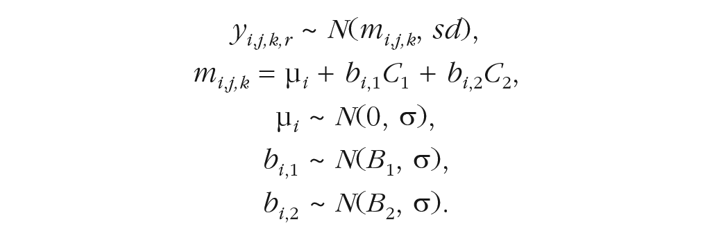
Here, yi, j,k,r is the observation of trial r in the design cell [ j,k] of subject i ( j and k are indices for the condition of Independent Variables 1 and 2, respectively). Each observation is sampled from a normal distribution with mean mi, j,k and standard deviation (sd) of 1. The subject’s mean in design cell [ j,k] is a linear combination of the subject’s intercept, or mean over all conditions, μ i , and the subject’s effects of the two independent variables. The independent variables are contrast coded [–0.5, +0.5], where C1 and C2 represent the contrast value of Independent Variables 1 and 2, respectively. The effect sizes of subject i for the two main effects are bi,1 and bi,2, respectively. 2 Each subject’s intercept is drawn from a normal distribution with mean of zero and standard deviation σ. The effects of the two predictor variables are drawn from normal distributions with means B1 and B2 and the same standard deviation σ. In mixed-model terms, the fixed effects are B1 and B2. They describe the population means of the effects of the predictors and are therefore called population-level effects in Bayesian statistics. The random effects are μ i , bi,1, and bi,2. They describe the deviation of each subject i from the population mean and are therefore called subject-level effects in the Bayesian terminology.
The simulation varied the effect size of the predictor of interest (Independent Variable 1) over four levels: B1 = 0, 0.25, 0.5, or 0.75. The second predictor had a constant effect size of 0.5. I also varied the size of the random effects over four levels of σ: .1, .25, .5, or 1. For each combination of B1 and σ, I ran 50 replications of the simulation.
The simulated data were analyzed on two levels of aggregation: unaggregated (i.e., the model predicted each individual trial), and aggregated on the level of the design cell (i.e., the model predicted each person’s mean in each design cell). For each level of aggregation, I applied four versions of an additive linear mixed model: The “RS” version included a random intercept and random slopes for both predictors as free parameters; the “no RS” version included only a random intercept. The “RS 1” version included a random slope only for Independent Variable 1 (i.e., the effect of interest), and the “RS 2 version” included a random slope only for Independent Variable 2. The models were run with the “lmBF” function of the BayesFactor package (Version 0.9.12.2; Morey & Rouder, 2015) for R (Version 3.6.2; R Core Team, 2020). I used the default prior settings of “lmBF” (i.e., Cauchy priors with scale = 0.5 for fixed effects and scale = 1 for random effects) and ran 100,000 Markov chain Monte Carlo (MCMC) iterations.
I gauged the evidence for the effect of interest by comparing the model including both predictors (Model 1) with a constrained model (Model 0) in which the predictor of interest (Independent Variable 1) was removed as a fixed effect. In the RS and RS 1 versions of the model, the constrained model still included the random effect of Predictor 1 because that model represents the null hypothesis that the population-level effect is zero, which does not necessarily mean that the effect is zero for each person.
Results
I first focus on results from the conditions in which the true effect of interest was zero. Figure 1 shows the BFs for the four model versions, for unaggregated data (left) and aggregated data (right), as a function of the true size of the random effects. Most BFs show evidence against the effect—these are the points below the red line in Figure 1. However, for the models that did not include a random slope for the effect of interest (i.e., no RS and RS 2), a substantial number of BFs reflected strong evidence in favor of the effect. The incidence and size of these BFs became larger as the true standard deviation of random effects increased. With unaggregated data, some of them were so large that I could fit them into the figure only by using a log10 scale. With aggregated data, BFs were much less extreme, reflecting less evidence both for and against the effect.
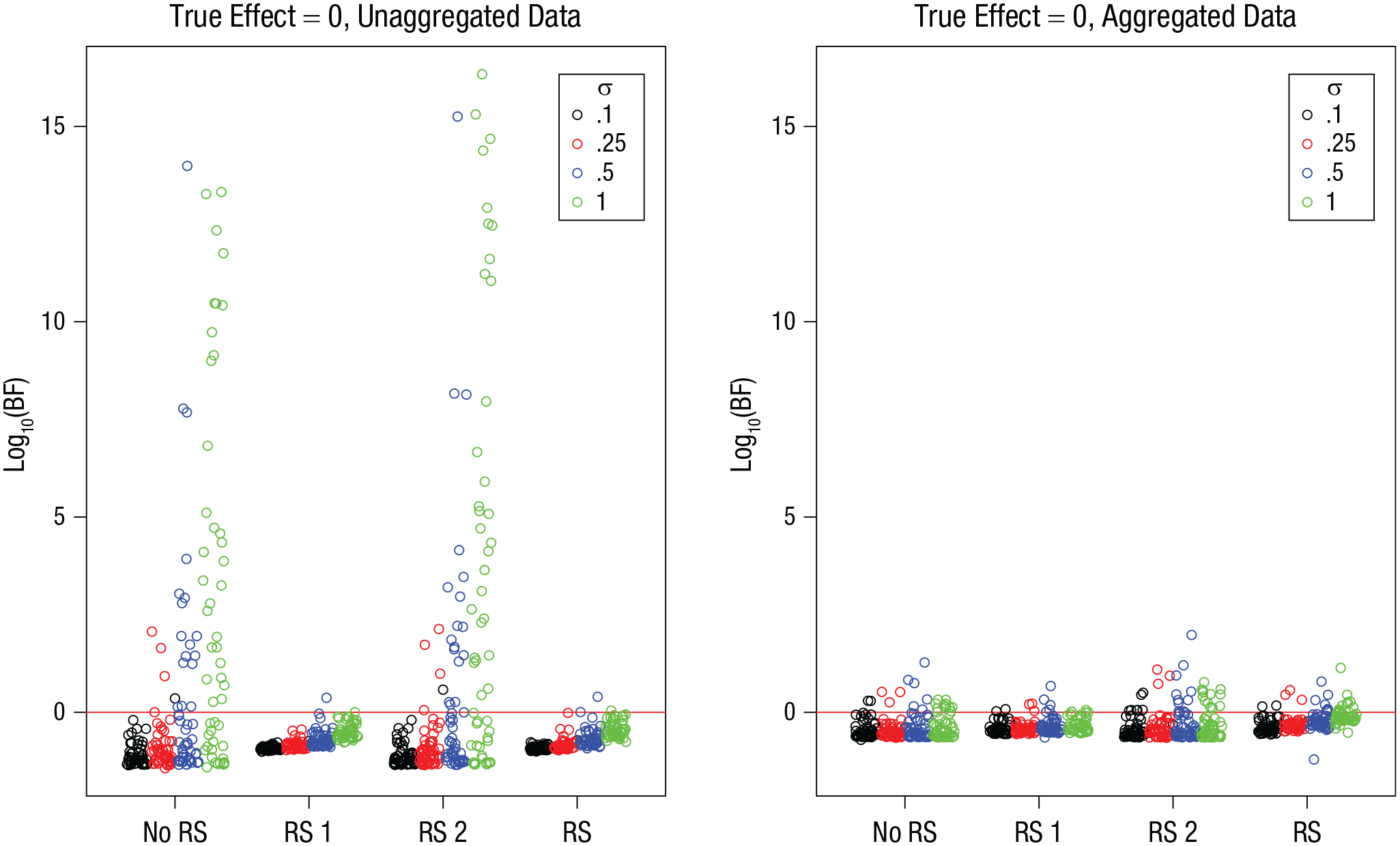
Simulation 1: Bayes factors (BFs) for the effect of interest when the true effect is zero, as a function of model version and standard deviation of random effects, σ. Results are shown separately for unaggregated data (left) and aggregated data (right). The “no RS” model version included no random slopes, the “RS 1” version included random slopes for the effect of interest, the “RS 2” version included random slopes for the other effect, and the “RS” version included random slopes for both effects. Each point is a BF from one simulation run. BFs are plotted on a log10 scale for visibility. BFs above the red line indicate evidence for the effect; those below the red line indicate evidence against the effect.
BFs estimate the strength of evidence for one model over another on a continuous scale, and there is no justifiable threshold for when to reach a conclusion in favor of one model or the other. Nevertheless, researchers often rely on rules of thumb for interpreting BFs in terms of categories of evidence strength. For instance, Kass and Raftery (1995), following Jeffreys (1961), proposed to interpret BFs between 3 and 10 as “substantial” evidence, and BFs between 10 and 100 as “strong” evidence. We can therefore ask what proportion of incorrect decisions researchers would be expected to make if they followed these recommendations for their conclusions.
The proportion of false positives—BFs reflecting evidence for a nonexistent effect—is given in Table 1, separately for mild false positives (BF > 3) and severe false positives (BF > 10). The proportions reflect the pattern in Figure 1: With unaggregated data, false positives were frequently observed when random slopes were omitted from the model and hardly ever when they were included. Aggregating the data flattened that effect, yielding intermediate rates of false positives, reduced only mildly by the inclusion of random slopes. The last row of the table shows the proportion of false positives when I followed the recommendation of Matuschek et al. (2017): For each simulation, I evaluated which random-effects structure (i.e., model versions RS 1, RS 2, RS, or no RS) was best supported by the data and kept the BF for the effect of interest from the best-supported model version. This approach was more successful in avoiding false positives than always omitting random slopes, although it was not as good as always including them.
Proportion of Bayes Factors (BFs) in Simulation 1 Reflecting Evidence for the Effect of Interest When the True Effect Was Zero

Note: For each model, results are shown separately for unaggregated data and aggregated data. Within each type of data, probabilities are further broken down for mild false positives (BF > 3) and severe false positives (BF > 10). The “no RS” model version included no random slopes, the “RS 1” version included random slopes for the effect of interest, the “RS 2” version included random slopes for the other effect, and the “RS” version included random slopes for both effects. For the “RS (evidence)” version, the inclusion of random effects was conditional on evidence supporting them.
Figure 2 presents a more fine-grained analysis of the BFs when the true effect was zero. Because of sampling noise, the sample effect deviated from the true effect, and the more it did, the more the BF was pushed in the direction of evidence for the effect. This bias was much stronger when random slopes were not included in the model. This effect can be understood as follows. When the size of the effect differs between subjects, then sampling noise is driven in part by these individual differences: For instance, when the sample happens to predominantly include subjects with positive effects, the sample effect will be positive. A model including random slopes represents this sampling noise adequately, whereas a model without a random slope tends to misattribute it to the fixed effect of the predictor and, therefore, yields false evidence for that effect.
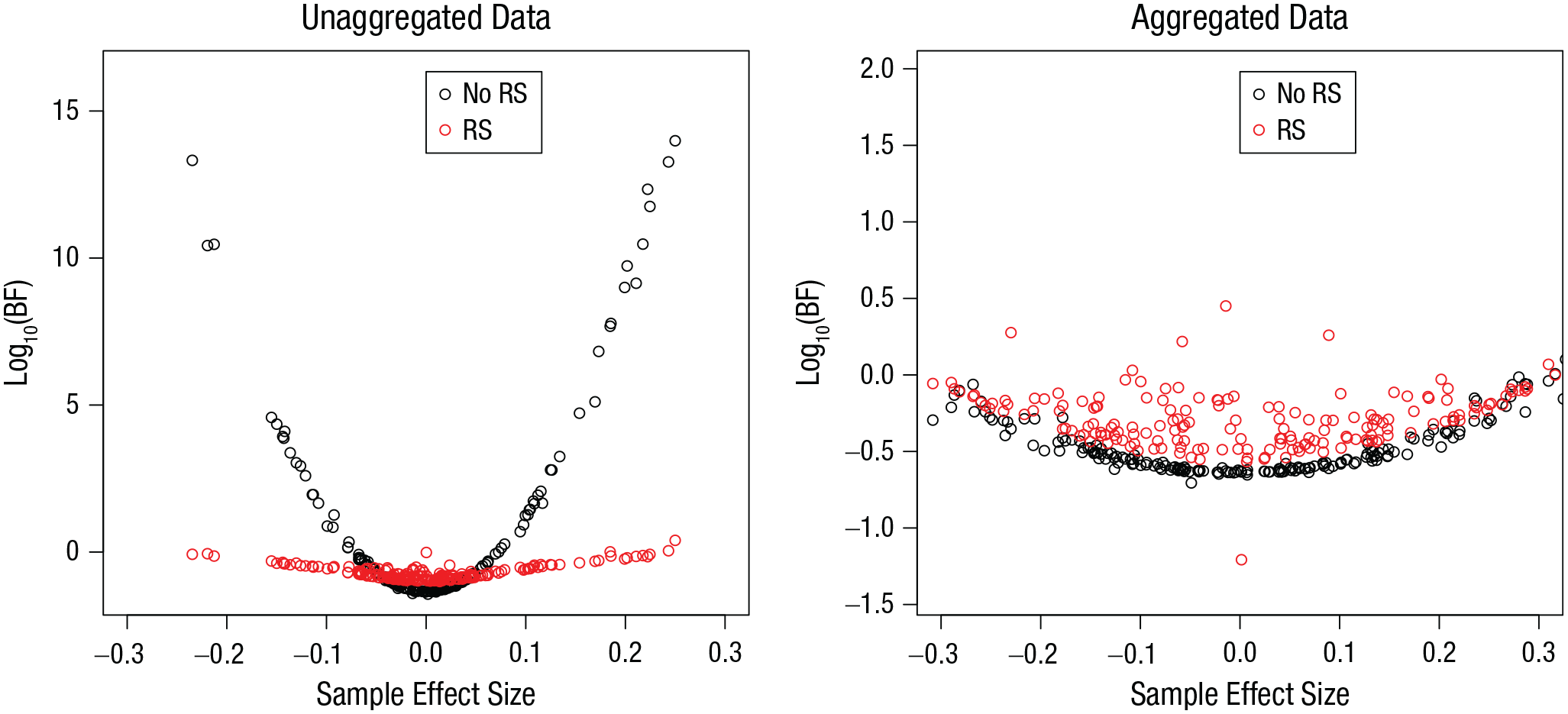
Simulation 1: Bayes factors (BFs) from simulations in which the effect of interest was zero, as a function of sample effect size and model version. Results are shown separately for unaggregated data (left) and aggregated data (right). The “no RS” model version included no random slopes, and the “RS” version included random slopes for both effects. Note the scale difference of the y-axis between graphs.
The reason why aggregation substantially mitigates the bias is this: In the unaggregated data, the deviation of a subject’s effect from the mean effect in the population is reflected by n data points per design cell. This sets the systematic deviation of that subject from the mean clearly apart from random measurement error (i.e., trial-by-trial variation). In contrast, in the aggregated data, the variability of the effect between subjects is represented by only one data point per cell for each subject and, thus, is barely distinguishable from within-subjects measurement error. 3 The within-subjects measurement error is accommodated in the model by the standard deviation of the normal distribution of individual observations. It provides sufficient variability to accommodate the between-subjects variability of effects in the aggregated data. In the unaggregated data, the standard deviation is bound to reflect only the trial-by-trial variability within each subject, missing the between-subjects variation.
Turning now to the simulations in which there was a true effect, I show in Figure 3 the BFs for each model version as a function of the size of the true effect. Unsurprisingly, the BFs increased with the true effect size. For unaggregated data, the BFs were much larger in model versions excluding the random slope of the effect of interest—in fact, for the largest effect size, most of them were so large that they exceeded the figure boundary. With aggregated data, all the BFs were in a more modest range.
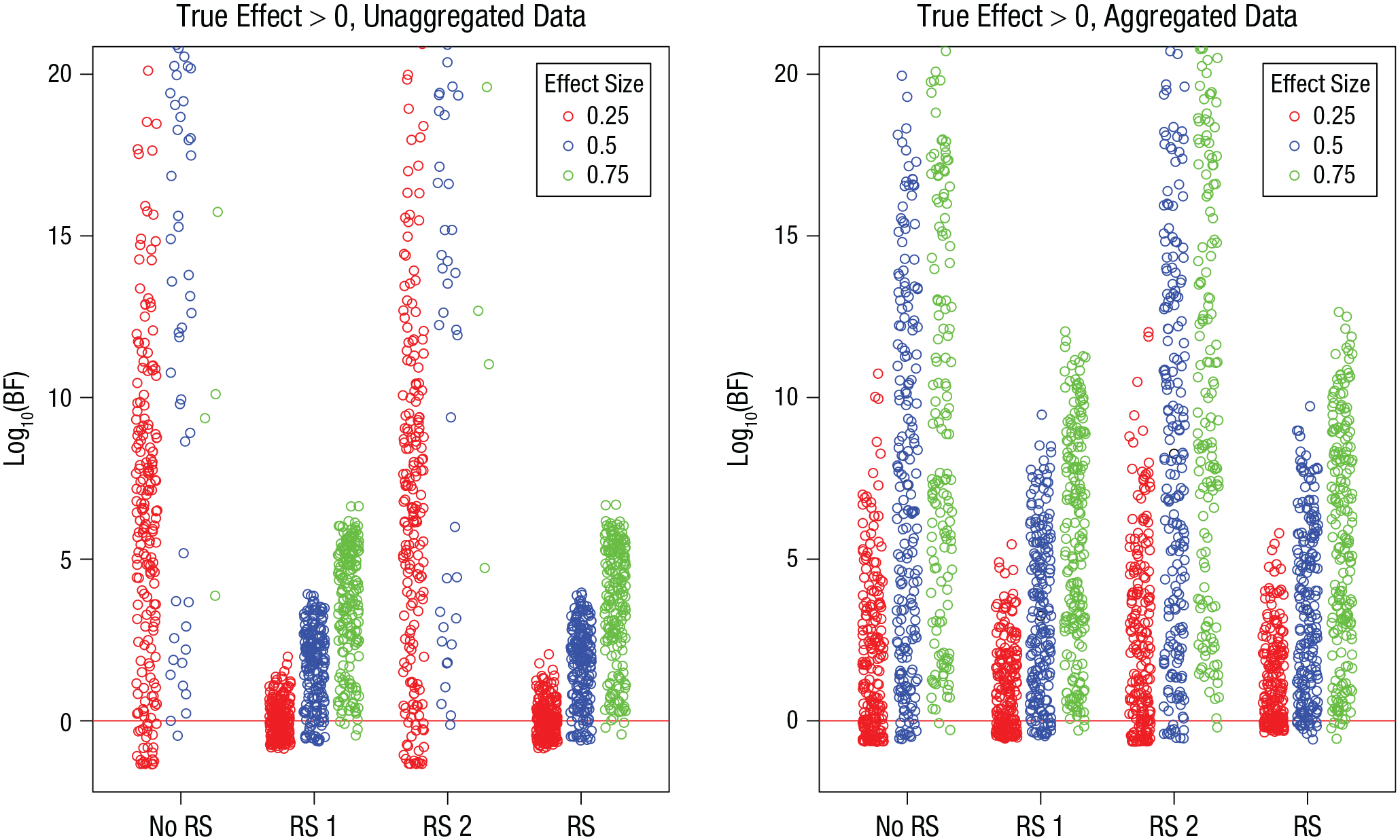
Simulation 1: Bayes factors (BFs) from simulations in which the effect of interest was greater than 0, as a function of model version and true effect size. Results are shown separately for unaggregated data (left) and aggregated data (right). The “no RS” model version included no random slopes, the “RS 1” version included random slopes for the effect of interest, the “RS 2” version included random slopes for the other effect, and the “RS” version included random slopes for both effects. Each point is a BF from one simulation run. BFs are plotted on a log10 scale for visibility. BFs above the red line indicate evidence for the effect; those below the red line indicate evidence against the effect.
Table 2 shows the proportion of simulations returning a miss (i.e., a BF < 3, which is ambiguous evidence) or a false negative (i.e., a BF < 0.33, which is evidence for the null hypothesis), on the assumption that researchers interpret evidence that is at least “substantial” (Kass & Raftery, 1995) to reach a conclusion in favor of a hypothesis. In the unaggregated data, misses and false negatives occurred more often when random slopes for the effect of interest were included (RS 1 and RS models). However, when the inclusion of random effects was conditional on evidence supporting them—“RS (evidence)” model—their prevalence was cut in half. In the aggregated data, the inclusion or omission of random slopes made less of a difference: Compared with the unaggregated data, there were more misses without random slopes in the models and fewer with them; false negatives were rare.
Proportion of Bayes Factors (BFs) in Simulation 1 Reflecting Ambiguous Evidence or Evidence Against the Effect of Interest When There Was a True Effect (Effect Sizes = 0.25, 0.5, and 0.75 Combined)
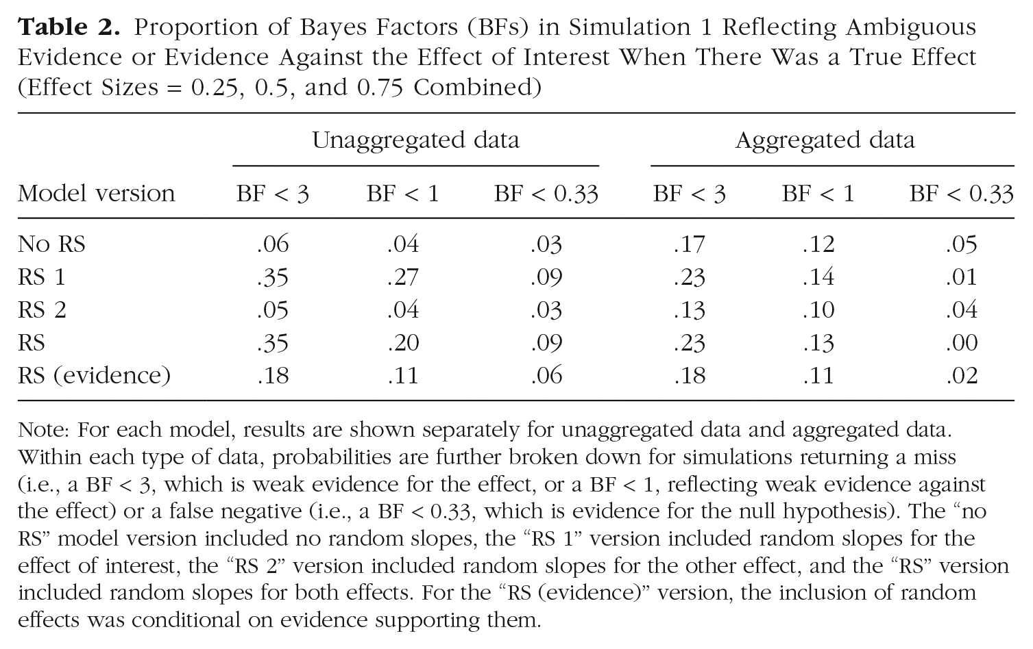
Note: For each model, results are shown separately for unaggregated data and aggregated data. Within each type of data, probabilities are further broken down for simulations returning a miss (i.e., a BF < 3, which is weak evidence for the effect, or a BF < 1, reflecting weak evidence against the effect) or a false negative (i.e., a BF < 0.33, which is evidence for the null hypothesis). The “no RS” model version included no random slopes, the “RS 1” version included random slopes for the effect of interest, the “RS 2” version included random slopes for the other effect, and the “RS” version included random slopes for both effects. For the “RS (evidence)” version, the inclusion of random effects was conditional on evidence supporting them.
Discussion
Simulation 1 showed that the pernicious effect of random slopes in misspecified models that Barr et al. (2013) pointed out for frequentist mixed models also applies to Bayesian mixed models. When there are true individual differences in the effects of interest, and these individual differences are not represented in the models as random slopes, there is a high risk of false positives, including BFs of a size that is considered to be decisive evidence. This risk can be mitigated in two ways. The first and most effective solution is to include the random slopes in the data, at least when there is evidence for them. The second, less effective solution is to aggregate the data within design cells. Both solutions come with a price: They increase the chance of missing a true effect and of even obtaining evidence against such an effect (i.e., a false negative), although that evidence was hardly ever strong (i.e., BFs < 0.1 were very rare). The best compromise appears to be to use unaggregated data and to include random slopes in the models only if a separate model comparison provides evidence for them.
Simulation 2: ANOVA With Many Design Cells
Simulation 1 showed that the problem of false positives when ignoring random slopes is mitigated substantially with aggregated data. The reason for that mitigation was that, with the aggregated data, each subject was represented with only two data points at each level of the predictor of interest—one mean for each level of the other predictor. Therefore, the aggregated data did not contain much evidence for distinguishing the random slopes from measurement noise. If this analysis is correct, then the problem of false positives should become more severe in aggregated data as the number of design cells—in particular, the number of levels of independent variables other than the one of focal interest—increases. To test this effect, I used the same basic setup in Simulation 2 as in Simulation 1 but varied the number of levels of Independent Variable 2.
Method
Simulation 2 was like Simulation 1, with one important modification: I varied the number of levels of Independent Variable 2 over four levels: two, four, six, and 10. The variable of interest, Independent Variable 1, still had two levels. To simplify the simulations, I used only one level of true random slopes, σ = .5, and only one level of a true effect, effect size = 0.5. Each simulation was run with 20 subjects and with 30 trials per design cell.
Results
Figure 4 shows the BFs for the simulations in which the true effect was zero. As in Simulation 1, there was a sizable number of BFs in favor of an effect when random slopes of the variable of interest (Predictor 1) were omitted. As expected, the prevalence and size of these BFs increased as the number of levels of Independent Variable 2 increased. This led to a nonnegligible number of false positives also in the aggregated data, as shown in Table 3.
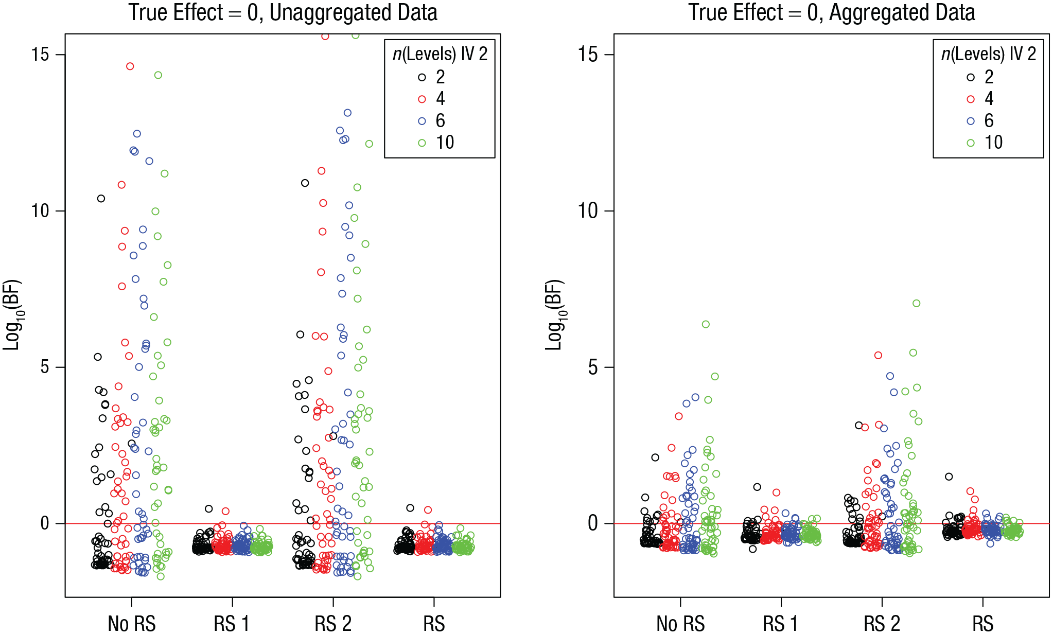
Simulation 2: Bayes factors (BFs) for the effect of interest when the true effect is zero, as a function of model version and number of levels of Independent Variable (IV) 2. Results are shown separately for unaggregated data (left) and aggregated data (right). The “no RS” model version included no random slopes, the “RS 1” version included random slopes for the effect of interest, the “RS 2” version included random slopes for the other effect, and the “RS” version included random slopes for both effects. Each point is a BF from one simulation run. BFs are plotted on a log10 scale for visibility (some extreme values are cut off at the top). BFs above the red line indicate evidence for the effect; those below the red line indicate evidence against the effect.
Proportion of Bayes Factors (BFs) in Simulation 2 Reflecting Evidence for the Effect of Interest When the True Effect Was Zero
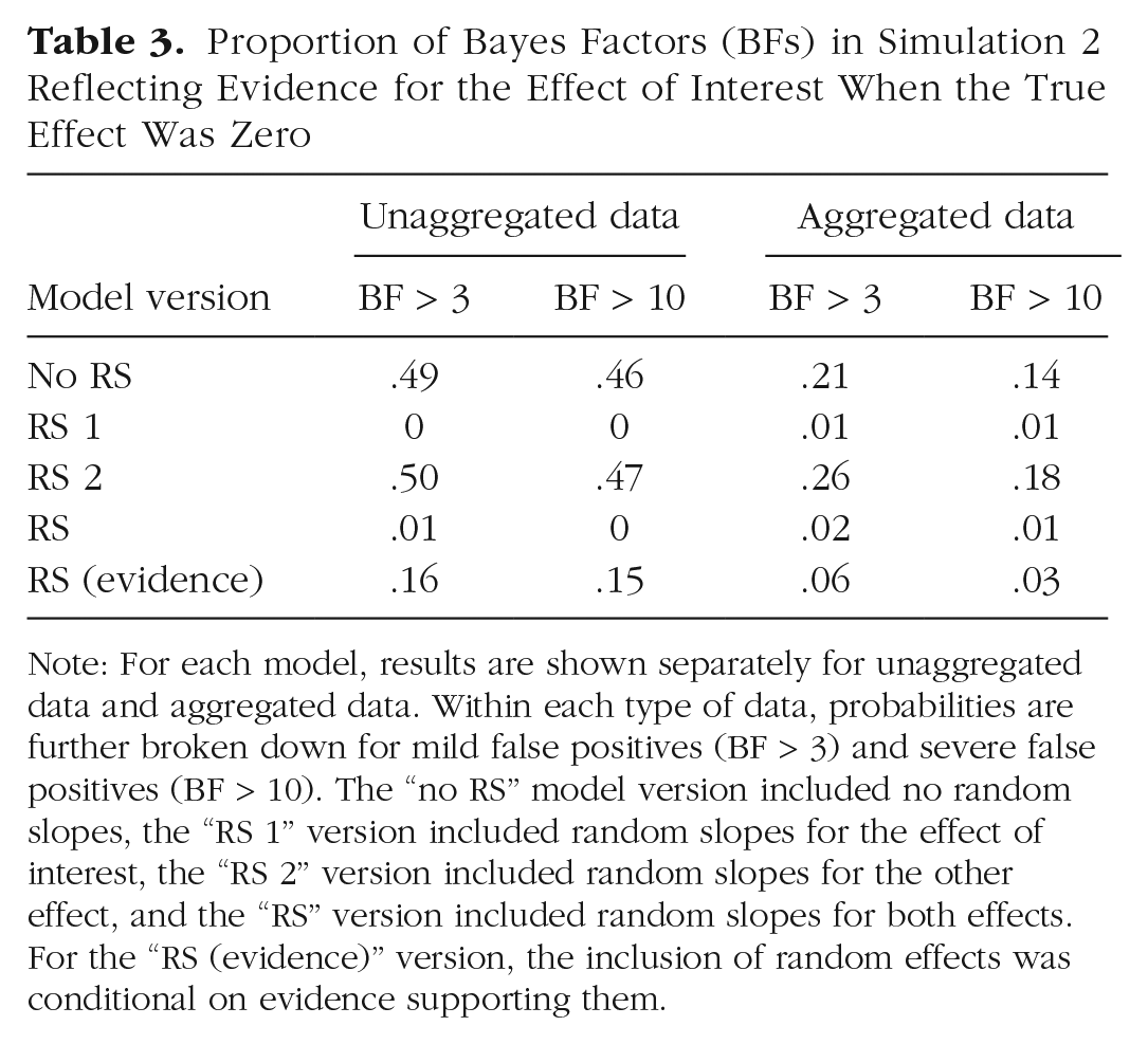
Note: For each model, results are shown separately for unaggregated data and aggregated data. Within each type of data, probabilities are further broken down for mild false positives (BF > 3) and severe false positives (BF > 10). The “no RS” model version included no random slopes, the “RS 1” version included random slopes for the effect of interest, the “RS 2” version included random slopes for the other effect, and the “RS” version included random slopes for both effects. For the “RS (evidence)” version, the inclusion of random effects was conditional on evidence supporting them.
Figure 5 shows the BFs for the simulation runs in which the true effect was 0.5. In the unaggregated data, the models omitting the random slopes of Predictor 1 produced BFs so huge that they were off the figure’s scale.
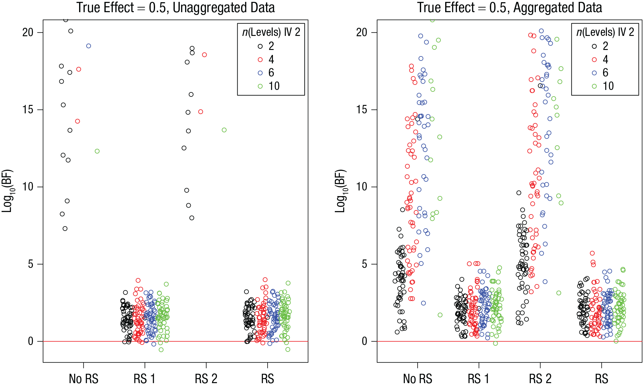
Simulation 2: Bayes factors (BFs) from simulations in which the effect of interest was greater than 0, as a function of model version and number of levels of Independent Variable (IV) 2. Results are shown separately for unaggregated data (left) and aggregated data (right). The “no RS” model version included no random slopes, the “RS 1” version included random slopes for the effect of interest, the “RS 2” version included random slopes for the other effect, and the “RS” version included random slopes for both effects. Each point is a BF from one simulation run. BFs are plotted on a log10 scale for visibility (some extreme values are cut off at the top). BFs above the red line indicate evidence for the effect; those below the red line indicate evidence against the effect.
The proportion of misses and false negatives is given in Table 4. This proportion was lower than in Simulation 1 for two reasons: Simulation 2 did not include the small effect size of 0.25, and it included simulations of designs with more cells; more cells led to more trials to inform the effect of interest because I held the number of trials per cell constant.
Proportion of Bayes Factors (BFs) in Simulation 2 Reflecting Ambiguous Evidence or Evidence Against the Effect of Interest When There Was a True Effect (Effect Size = 0.5)
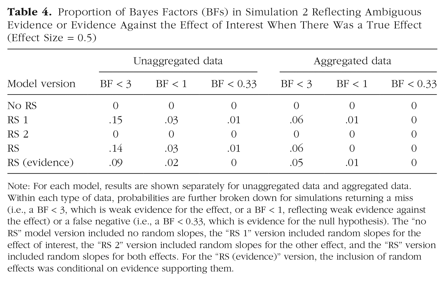
Note: For each model, results are shown separately for unaggregated data and aggregated data. Within each type of data, probabilities are further broken down for simulations returning a miss (i.e., a BF < 3, which is weak evidence for the effect, or a BF < 1, reflecting weak evidence against the effect) or a false negative (i.e., a BF < 0.33, which is evidence for the null hypothesis). The “no RS” model version included no random slopes, the “RS 1” version included random slopes for the effect of interest, the “RS 2” version included random slopes for the other effect, and the “RS” version included random slopes for both effects. For the “RS (evidence)” version, the inclusion of random effects was conditional on evidence supporting them.
Discussion
The take-home message from Simulation 2 is that, even with aggregated data, the risk of false positives when true random slopes are omitted from the model becomes uncomfortably high when the experimental design becomes more complex (i.e., each level of the predictor of interest is represented by a larger number of design cells).
Simulation 3: Multilevel Regression
With this simulation, I aimed to answer two questions. First, what is the effect of omitting random slopes of continuous predictors in regression models from a model when such effects are actually in the data? Second, what is the effect of omitting correlations between random slopes when such correlations are in the data?
Method
I simulated a within-subjects design with two predictor variables that varied over five levels on a continuous dimension, such as five list lengths combined with five retention intervals in a memory experiment. This means that the scale was at least ordinal, and the five levels were ordered from the smallest to the largest. The two predictors were not fully crossed but, rather, varied randomly and independently across the 150 trials simulated for each subject, with the constraint that for each predictor, each value was realized equally often (i.e., 30 times). For both the data-generating model and the model fitted to the data, I used z-standardized variables with five equidistant values as predictors, so that the effect size was standardized. The effect size of the first predictor—the predictor of interest in the model comparisons—was either 0 or 0.25. The effect size for the second predictor was always 0.25.
Two variables were varied across simulations: the standard deviation of the random slopes of both predictors (σ = .1, .25, .5, or 1) and the correlation between the two predictors across subjects (r = 0, .2, .5, or .7). For each combination of these variables, I ran 40 replications of the simulation with 20 subjects each. 4
For each simulation, I tested the effect of the first predictor by comparing a model including both predictors as fixed effects with one in which the first predictor’s fixed effect was removed. This was done for three model versions: The “no RS” version included no random slopes, the “RS” version included uncorrelated random slopes for the two predictors, and the “RS + Corr” version included the two random slopes and their correlation as free parameters. The models were applied only to unaggregated data because this is the situation in which Simulation 1 revealed the larger effect of random slopes. Because the BayesFactor package does not support random slopes for continuous (numerical) predictors, I used the brms package (Version 2.15.0; Bürkner, 2017) for running the models and the bridgesampling package (Version 1.1-2; Gronau et al., 2020) for estimating the BFs. The models were run with three chains of 10,000 iterations each (including 1,000 warm-up iterations). The priors for the standardized effect sizes were default Cauchy priors with scale 0.5 (Rouder et al., 2012).
Results
Figure 6 shows the BFs for the simulations in which the true effect of interest was zero. As in Simulation 1, when random slopes were omitted from the models, there was a nonnegligible proportion of simulations that produced huge BFs in favor of the effect. The proportion of false positives is given in Table 5. The prevalence and size of BFs in favor of an effect increased as σ, the standard deviation of the true random slopes, increased. 5 When random slopes were included in the models, these false positives were strongly mitigated. This was the case regardless of whether a correlation between the random slopes was included.
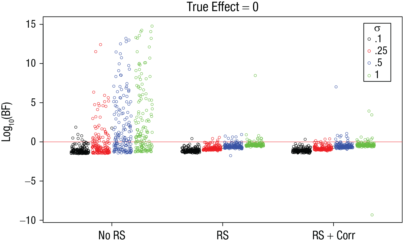
Simulation 3: Bayes factors (BFs) for the effect of interest when the true effect is zero, as a function of model version and standard deviation of random effects, σ. The “no RS” model version included no random slopes, the “RS” version included random slopes for both effects, and the “RS + Corr” version included random slopes for both effects and the correlation between them. Each point is a BF from one simulation run. BFs are plotted on a log10 scale for visibility (some extreme values are cut off at the top). BFs above the red line indicate evidence for the effect; those below the red line indicate evidence against the effect.
Proportion of Bayes Factors (BFs) in Simulation 3 Reflecting Evidence for the Effect of Interest When the True Effect Was Zero
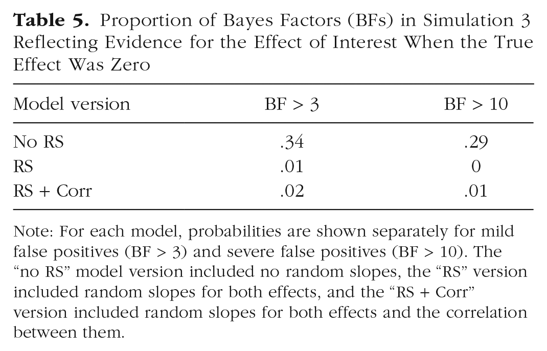
Note: For each model, probabilities are shown separately for mild false positives (BF > 3) and severe false positives (BF > 10). The “no RS” model version included no random slopes, the “RS” version included random slopes for both effects, and the “RS + Corr” version included random slopes for both effects and the correlation between them.
Figure 7 shows the same BFs as a function of the true size of the correlation: This variable had no discernible effect on the false-positive rate or size. Table 5 summarizes the proportion of false positives for the three model versions, and Table 6 shows the proportion of misses and of false negatives. They show again that including random slopes in the models reduces the false-positive rate but at the cost of increasing misses of true effects and even increasing false negatives (although the latter still remained at a low level). Whether or not the correlation was included did not matter.
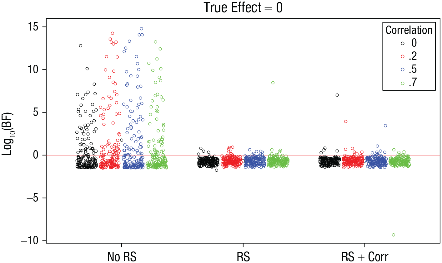
Simulation 3: Bayes factors (BFs) for the effect of interest when the true effect is zero, as a function of model version and the size of the correlation between the random slopes of the two independent variables. The “no RS” model version included no random slopes, the “RS” version included random slopes for both effects, and the “RS + Corr” version included random slopes for both effects and the correlation between them. Each point is a BF from one simulation run. BFs are plotted on a log10 scale for visibility. BFs above the red line indicate evidence for the effect; those below the red line indicate evidence against the effect.
Proportion of Bayes Factors (BFs) in Simulation 3 Reflecting Ambiguous Evidence or Evidence Against the Effect of Interest When the True Effect Was 0.25
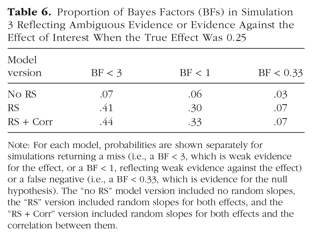
Note: For each model, probabilities are shown separately for simulations returning a miss (i.e., a BF < 3, which is weak evidence for the effect, or a BF < 1, reflecting weak evidence against the effect) or a false negative (i.e., a BF < 0.33, which is evidence for the null hypothesis). The “no RS” model version included no random slopes, the “RS” version included random slopes for both effects, and the “RS + Corr” version included random slopes for both effects and the correlation between them.
Discussion
Simulation 3 confirmed what was already shown in the previous two simulations: In mixed regression models, just as in ANOVA models, omitting random slopes from models when they are in the data increases the risk of false positives with potentially enormous BFs in favor of a nonexistent effect. The new result of Simulation 3 is that omitting the correlations between random slopes when they are in the data is innocuous.
Simulation 4: Effects of Sample Size and Number of Trials
For this simulation, I returned to an ANOVA design and addressed a question that probably every experimenter who has read this far has wondered about: How does the number of subjects, and the number of trials per subject, affect the results from the previous simulations?
Method
Simulation 4 repeated the basic 2 × 2 ANOVA design of Simulation 1, with the following changes. I orthogonally varied the sample size (N = 20, 30, 40, or 50) and the number of trials per design cell (n = 20, 30, 40, 60, or 90). The true size of random slopes was held constant, σ = .5. For true effects, I simulated only an effect size of 0.25 because a relatively small effect size should be most informative about how N and n affect the risk of misses or false negatives.
Results
The distribution of BFs for simulations in which the true effect was zero is shown in Figure 8 as a function of sample size and in Figure 9 as a function of the number of trials. Table 7 gives the proportions of false positives. It is clear that neither increasing the sample size nor increasing the number of trials has a mitigating effect on the prevalence or the size of false positives. If anything, more data makes the problem worse, although the effect is modest at best.
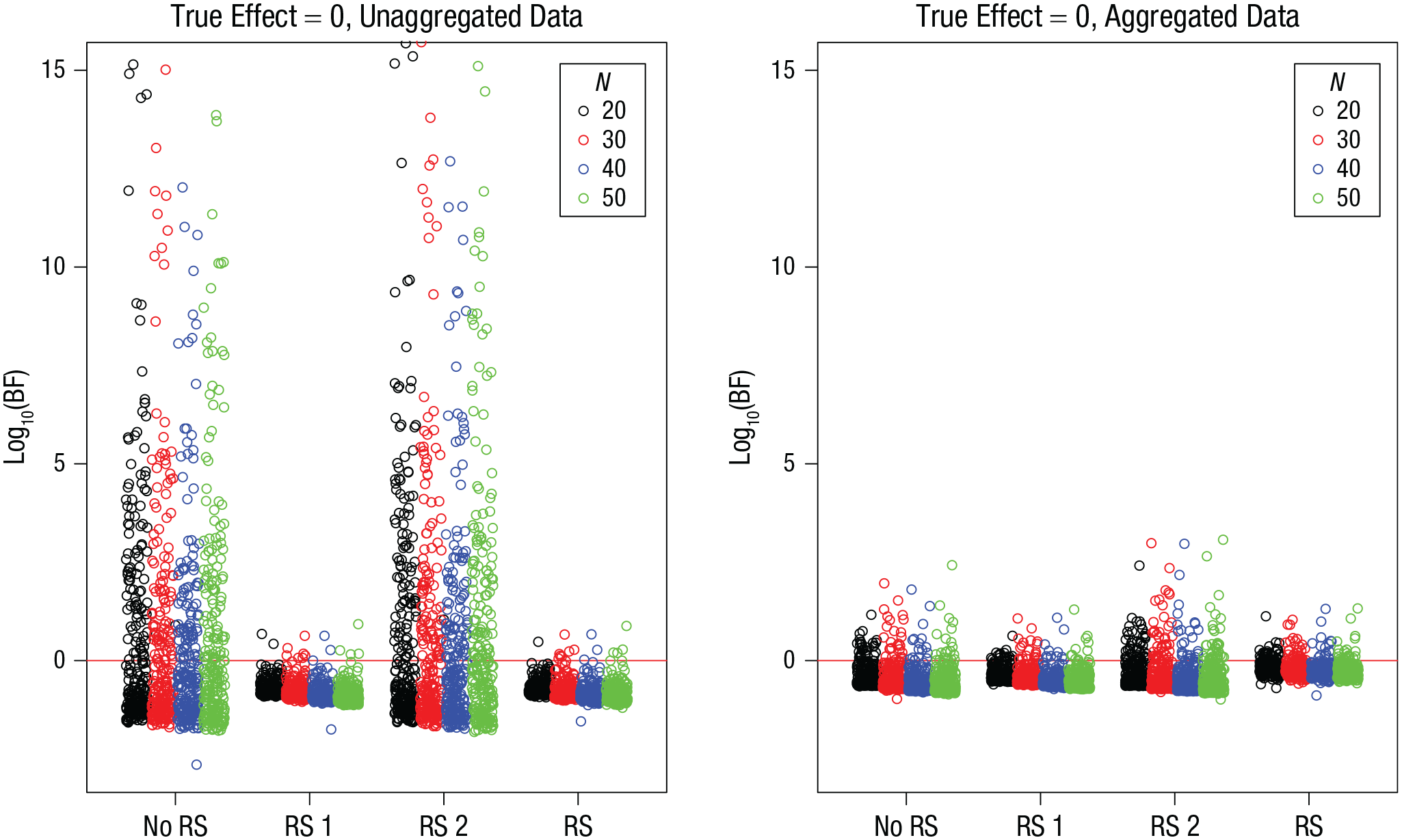
Simulation 4: Bayes factors (BFs) for the effect of interest when the true effect is zero, as a function of model version and sample size, N. Results are shown separately for unaggregated data (left) and aggregated data (right). The “no RS” model version included no random slopes, the “RS 1” version included random slopes for the effect of interest, the “RS 2” version included random slopes for the other effect, and the “RS” version included random slopes for both effects. Each point is a BF from one simulation run. BFs are plotted on a log10 scale for visibility (some extreme values are cut off at the top). BFs above the red line indicate evidence for the effect; those below the red line indicate evidence against the effect.
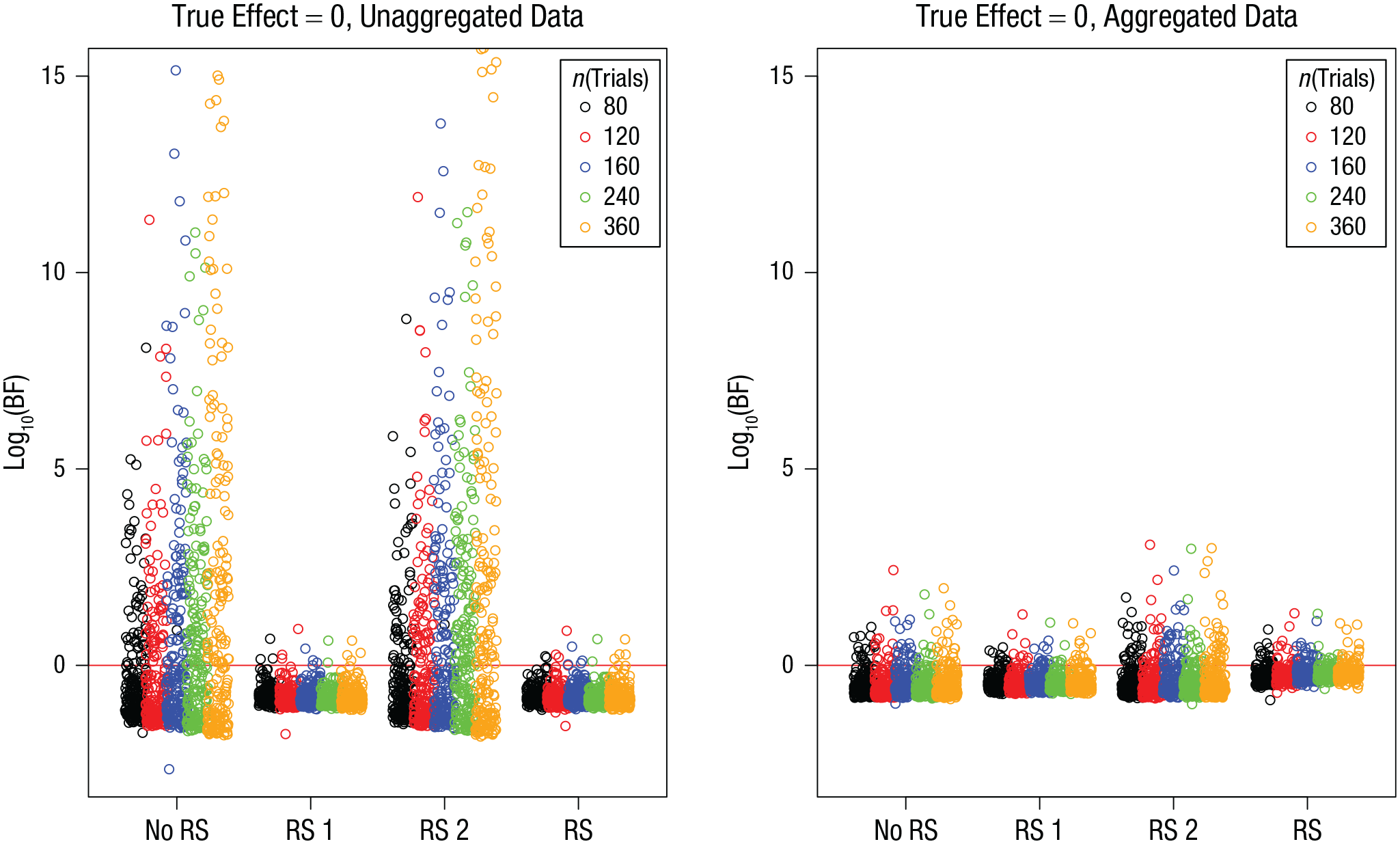
Simulation 4: Bayes factors (BFs) for the effect of interest when the true effect is zero, as a function of model version and number of trials per subject. Results are shown separately for unaggregated data (left) and aggregated data (right). The “no RS” model version included no random slopes, the “RS 1” version included random slopes for the effect of interest, the “RS 2” version included random slopes for the other effect, and the “RS” version included random slopes for both effects. Each point is a BF from one simulation run. BFs are plotted on a log10 scale for visibility (some extreme values are cut off at the top). BFs above the red line indicate evidence for the effect; those below the red line indicate evidence against the effect.
Proportion of Bayes Factors (BFs) in Simulation 4 Reflecting Evidence for the Effect of Interest When the True Effect Was Zero
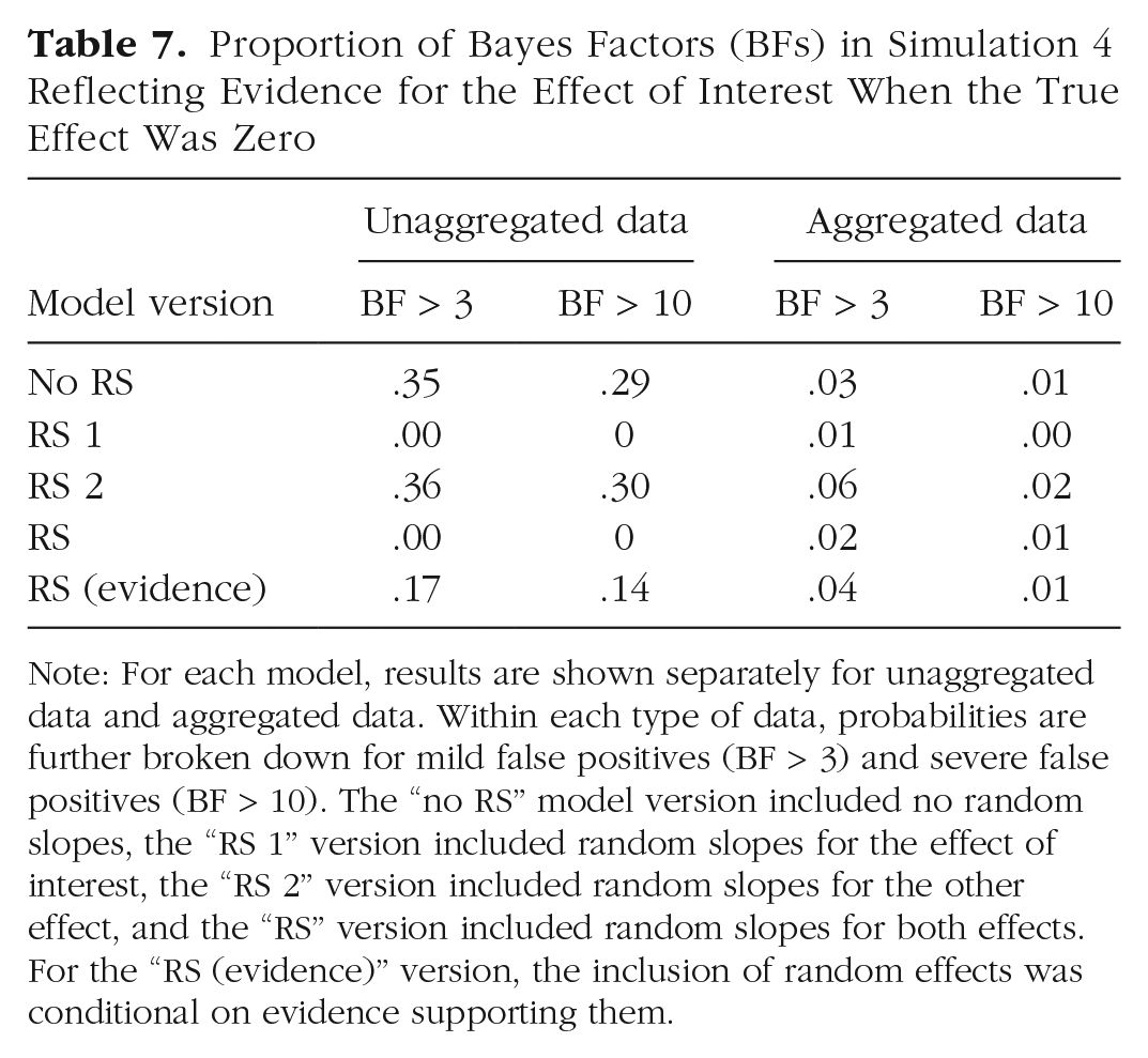
Note: For each model, results are shown separately for unaggregated data and aggregated data. Within each type of data, probabilities are further broken down for mild false positives (BF > 3) and severe false positives (BF > 10). The “no RS” model version included no random slopes, the “RS 1” version included random slopes for the effect of interest, the “RS 2” version included random slopes for the other effect, and the “RS” version included random slopes for both effects. For the “RS (evidence)” version, the inclusion of random effects was conditional on evidence supporting them.
Figures 10 and 11 present the BFs for simulations with a true effect, and Table 8 summarizes the proportion of misses and of false negatives from these simulations. As in Simulations 1 to 3, including random slopes of the effect of interest increased the probability of missing the true effect and of even obtaining (modest) evidence against it. In analogy to the effect of sample size on statistical power in frequentist significance testing, we should expect sample size, and probably also the number of trials, to reduce that risk. This is indeed the case, as shown in Table 9, which breaks down the proportion of misses by sample size and number of trials. The proportion of misses—defined here as BF < 1—in models that include random slopes is clearly reduced with increasing sample size. The number of trials appears to matter less. However, when one looks at the scenario in which the random-effects structure of the model is determined empirically, including only those random slopes that are supported by the data (lower half of Table 9), increasing the number of trials noticeably reduces the proportion of misses.
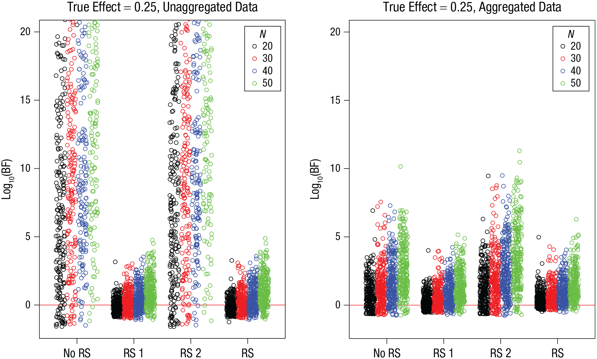
Simulation 4: Bayes factors (BFs) for the effect of interest when the true effect is 0.25, as a function of model version and sample size, N. Results are shown separately for unaggregated data (left) and aggregated data (right). The “no RS” model version included no random slopes, the “RS 1” version included random slopes for the effect of interest, the “RS 2” version included random slopes for the other effect, and the “RS” version included random slopes for both effects. Each point is a BF from one simulation run. BFs are plotted on a log10 scale for visibility (some extreme values are cut off at the top). BFs above the red line indicate evidence for the effect; those below the red line indicate evidence against the effect.
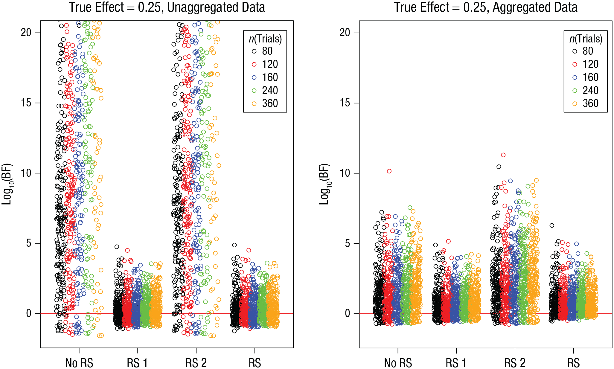
Simulation 4: Bayes factors (BFs) for the effect of interest when the true effect is 0.25, as a function of model version and number of trials per subject. Results are shown separately for unaggregated data (left) and aggregated data (right). The “no RS” model version included no random slopes, the “RS 1” version included random slopes for the effect of interest, the “RS 2” version included random slopes for the other effect, and the “RS” version included random slopes for both effects. Each point is a BF from one simulation run. BFs are plotted on a log10 scale for visibility (some extreme values are cut off at the top). BFs above the red line indicate evidence for the effect; those below the red line indicate evidence against the effect.
Proportion of Bayes Factors (BFs) in Simulation 4 Reflecting Ambiguous Evidence or Evidence Against the Effect of Interest When There Was a True Effect (Effect Size = 0.25)
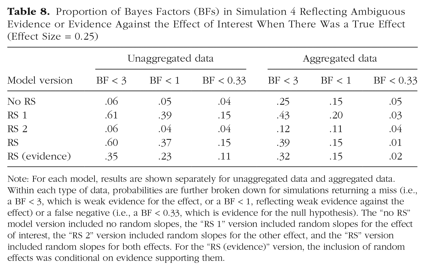
Note: For each model, results are shown separately for unaggregated data and aggregated data. Within each type of data, probabilities are further broken down for simulations returning a miss (i.e., a BF < 3, which is weak evidence for the effect, or a BF < 1, reflecting weak evidence against the effect) or a false negative (i.e., a BF < 0.33, which is evidence for the null hypothesis). The “no RS” model version included no random slopes, the “RS 1” version included random slopes for the effect of interest, the “RS 2” version included random slopes for the other effect, and the “RS” version included random slopes for both effects. For the “RS (evidence)” version, the inclusion of random effects was conditional on evidence supporting them.
Proportion of Bayes Factors Less Than 1 in Simulation 4 When There Was a True Effect, as a Function of Sample Size and Number of Trials
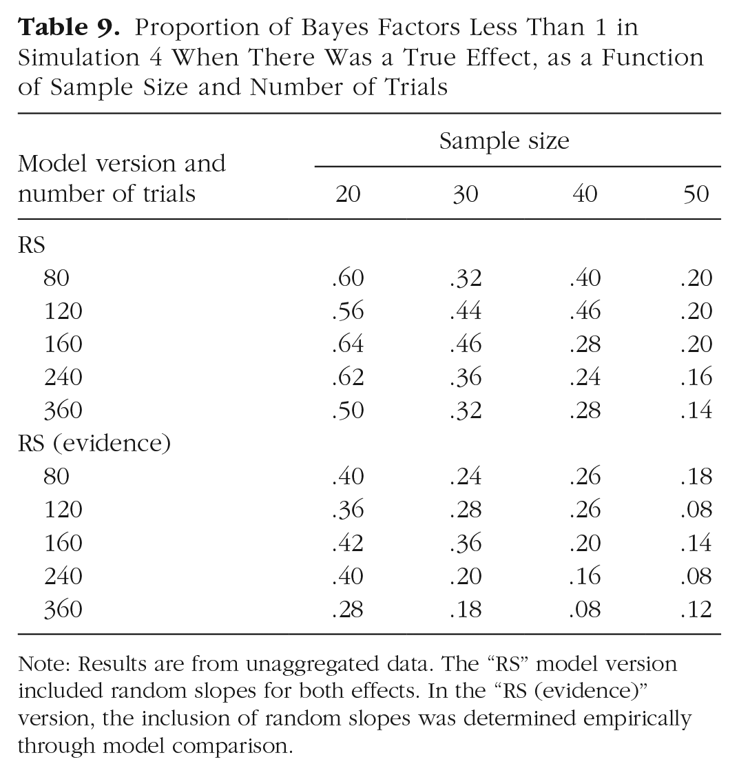
Note: Results are from unaggregated data. The “RS” model version included random slopes for both effects. In the “RS (evidence)” version, the inclusion of random slopes was determined empirically through model comparison.
Discussion
More data can fix many statistical problems but not the one identified here: When there are true individual differences in the effect of interest, but random slopes of that effect are omitted from the model, there is a substantial risk of BFs reflecting strong but wrong evidence for the effect. Neither increasing the sample size nor increasing the number of trials reduces that risk.
That said, increasing the sample size reduces the risk of missing a true effect. Increasing the number of trials can achieve that as well, although this benefit appears to be best leveraged when the random-effects structure of the model is determined empirically rather than always including all random slopes.
Simulation 5: BF Calibration
The final simulation addressed the question of whether the BFs estimated for a two-factorial ANOVA design are well calibrated, as opposed to biased, for three model-comparison approaches: always omitting random slopes, always including random slopes, and a parsimonious approach, including random slopes only if there is evidence for them. This simulation was inspired by the recent work of Schad et al. (2022) and followed their procedure.
In each simulation run, I sampled one of two models—the null model and the alternative model—according to the prior probability of each model. I sampled parameter values from the parameter priors of the chosen model, simulated data from it, and then estimated the BF for the effect of interest according to each of the three model-comparison approaches. From the BF, I computed the posterior probability of each model. If the BF is well calibrated, the posterior probabilities, averaged over all simulation runs, should closely approximate the models’ prior probabilities. In a simulation for a one-factorial design, Schad et al. (2022) found that the BF was well calibrated for models that included random slopes but was biased in favor of the alternative model if they did not, mirroring the present results. I expected to find the same result here. The question of most interest was whether the parsimonious model-comparison approach, including random slopes only if there is evidence for them in the data, would yield a well-calibrated BF.
Method
I used a 2 × 2 within-subjects ANOVA design as in Simulation 1, with 20 subjects and 30 trials per design cell. In each of 1,000 simulation runs, the null model or the alternative model was chosen with its prior probability, which I set to .5 for both models. Different from Simulation 1, the model parameters were not varied factorially but sampled from the parameter priors of the model. The parameter priors were those implemented in the BayesFactor package and described by Rouder et al. (2012), with one exception described below. When the alternative model was chosen, the fixed effects of both independent variables were drawn from the default prior on standardized effect sizes (i.e., Cauchy priors with scale = 0.5). When the null model was chosen, the fixed effect of the independent variable of interest was set to 0.
I simulated data from the chosen model with the sampled parameter values and then estimated the BF for the effect of interest with the BayesFactor package in three ways: always omitting random slopes (no RS), always including random slopes (RS), and using the most parsimonious model justified by the data (RS evidence). For the latter, I first tested for the random slopes by comparing the full model with a model excluding the random slopes of both independent variables. If the BF for random slopes exceeded 1, the subsequent test for the fixed effect of interest included those random slopes in the models; otherwise, it omitted the random slopes. The analyses were always conducted on unaggregated data.
Sampling the standard deviation of the random slopes from the prior proposed by Rouder et al. (2012) generated unrealistically large values, so that the BFs in favor of keeping the random slopes in the model were always huge. As a consequence, the parsimonious model-comparison approach could not be evaluated because random slopes would never be omitted. Therefore, I sampled the standard deviations of random slopes from a gamma prior with a shape of 2 and rate of 10 (implying a mean of 0.2), which yielded random slopes that were detected about half of the time. From the BF estimated with each of the three model-comparison approaches, I computed the posterior probabilities of the models as follows:
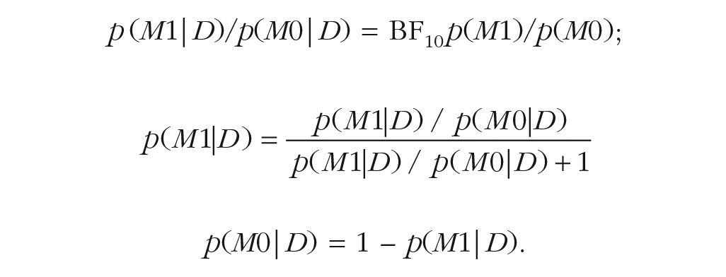
Results
The model-comparison approach omitting random slopes was not well calibrated: It returned an overly high posterior probability of the alternative model, p(M1|D) = .53, 95% confidence interval (CI) = [.50, .57]. The approach always including random slopes was well calibrated, p(M1|D) = .50, 95% CI = [.46, .53], as was the parsimonious approach including random slopes only when there was evidence for them, p(M1|D) = .51, 95% CI = [.48, .54]. Table 10 gives a breakdown of the posterior model probabilities by the true model generating the data. It shows that the bias in model comparisons always omitting random slopes comes from overestimating the posterior probability of M1 when the null model was true.
Mean Posterior Model Probabilities in Simulation 5 as a Function of the True Model (M0 or M1) and the Model-Comparison Approach
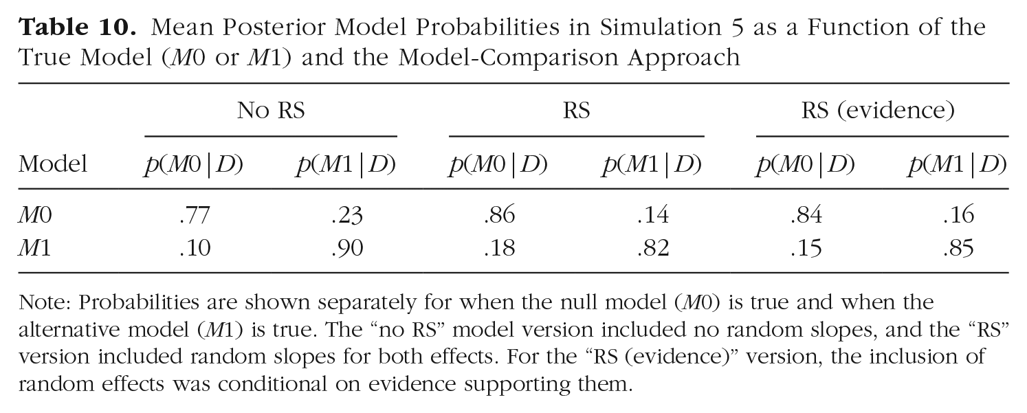
Note: Probabilities are shown separately for when the null model (M0) is true and when the alternative model (M1) is true. The “no RS” model version included no random slopes, and the “RS” version included random slopes for both effects. For the “RS (evidence)” version, the inclusion of random effects was conditional on evidence supporting them.
Discussion
The simulation-based calibration confirmed that always omitting random slopes results in a biased BF if random slopes are part of the data-generating process. The bias reflected in the averaged model posteriors might appear benign. This is in part because the standard deviations of the random slopes tended to be smaller than in the previous simulations. Nevertheless, there were still 7.4% false positives with BF greater than 10. Always including random slopes, as well as using the parsimonious model-comparison approach, yielded well-calibrated BFs at least for one common design. This is no guarantee that BFs for other designs or other experimental parameters (e.g., number of subjects and trials) are also well calibrated. To be sure that they are, researchers might consider running calibration simulations for their design.
Random Slopes in brms, BayesFactor, and JASP
On the practical side, including random slopes in Bayesian mixed models is not always straightforward. To the best of my knowledge, the three most popular software tools for running such models in psychology are the R packages brms (Bürkner, 2017) and BayesFactor (Morey & Rouder, 2015) and the free stand-alone application JASP (JASP Team, 2020).
The brms package gives users maximal flexibility in specifying their model, including the random-effects structure. The core function, “brm,” takes as the first argument a formula in the standard language of R, in which random effects can be specified. For instance, the following formula—using the general formula language for mixed models in R—describes a model with two main effects as fixed effects, together with the random intercept, and the random slopes of both predictors:
brm(formula = dv ~ iv1 + iv2 + (1 + iv1 + iv2 || id), . . .)
In plain English, the dependent variable (“dv”) is a function of the additive fixed effects of Independent Variables 1 and 2 (“iv1” and “iv2”). The random effects are added in parentheses, and the variable identifying the subject (“id”) is the unit of random variation. The expression before the double bar specifies a random intercept (1) and random slopes of the effects of iv1 and iv2. The double bar excludes correlations between random effects; a single bar is used to include them.
In the BayesFactor package, the “lmBF” function offers the same functionality for linear mixed models. The following code specifies the same model as above:
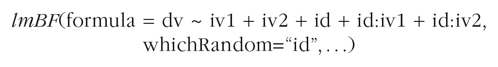
Here, the random effects are included in the formula in the same way as fixed effects, and the argument “whichRandom” is used to specify which predictors are to be treated as the units of random variation. One limitation of “lmBF” is that it does not reliably support random slopes of continuous predictors (i.e., predictors that are numerical variables rather than factors in R). This is why I could not run Simulation 3 with the BayesFactor package. The “anovaBF” function in the BayesFactor package is dedicated to ANOVA models. It includes random intercepts but no random slopes, and there is no option for the user to include the latter. Therefore, using the “anovaBF” function incurs a substantial risk of false positives, especially when the design has many within-subjects cells.
In JASP, users can choose between Bayesian ANOVAs and Bayesian mixed models. The “mixed models” function enables users to choose their random-effects structure. By default, random slopes and their correlations are included for all predictors. The “ANOVA” function, by contrast, includes only random intercepts, without any flexibility. The required data format enforces aggregation of data within each design cell; therefore, the risk of hugely inflated false-positive BFs is small. Nevertheless, running Bayesian within-subjects ANOVAs in JASP entails a nonnegligible risk of false-positive BFs, especially when the design has many cells. To confirm this conjecture, I ran a simple simulation of a 2 × 6 ANOVA design with the same specifications as Simulation 2 and a true effect of zero. Out of 100 simulated data sets, 32 yielded a BF greater than 3 for the effect, and 19 of them yielded a BF greater than 10.
General Discussion
As Bayesian statistics is gaining ground, we need to become aware of the potential pitfalls involved in using it. One potential pitfall is to use mixed-effects models to test hypotheses about effects on the population level without including random slopes in the model. If there are true individual differences in the effect of interest, this can lead to massively inflated evidence in favor of the effect on the population level, even if no such effect exists.
This result mirrors the one that Barr et al. (2013) reported for mixed-model comparisons in frequentist statistics, but the problem is more pervasive for Bayesian than for frequentist hypothesis testing. In frequentist statistics, the main tool for null-hypothesis testing in within-subjects designs is the within-subjects (or repeated measures) ANOVA. The F test for this ANOVA includes the variance generated by random slopes—together with measurement error—in the error term and thereby automatically accounts for their effect. Therefore, significance testing based on the F statistic from within-subjects ANOVA does not lead to inflated false-positive rates. By contrast, hypothesis testing with Bayesian ANOVAs (Rouder et al., 2012), as built into the BayesFactor package and JASP, relies on model comparisons and therefore gives rise to a substantial risk of exaggerated evidence for nonexistent effects.
Readers might think that the results of the present simulations are trivial because they merely show that using misspecified models leads to erroneous conclusions. It is not that simple. Except in the idealized environment of a simulated ground truth, models are always simplified descriptions of reality, and yet they are often useful for inferences (Box, 1979). For instance, the comparison of a linear model with a null model is useful to detect a monotonic trend even if it is nonlinear. We need to find out which simplifications we can afford without undercutting their usefulness. It turns out that we cannot afford to simplify away random slopes. It could have turned out otherwise: A comparison of two models omitting random slopes that are actually warranted by the data is not obviously biased a priori because both models suffer the same misspecification.
What can we do to minimize the risk of exaggerated evidence for nonexistent effects? One obvious solution is to always include random slopes in the models that we compare. This comes with two costs. One is that the chance of obtaining convincing evidence (i.e., large BFs) for a true effect is reduced substantially. The other is that the models run much longer. A compromise could be to include only those random slopes that are warranted by the data. The rationale behind this approach is to first search for the most parsimonious model of the random effects in the data, thereby culling any excess flexibility in the model, before turning to model comparisons testing the fixed effects of interest (Matuschek et al., 2017). This approach reduces the risk of false positives, but not as much as always including random slopes (this became most apparent in Simulations 2 and 4). It also reduces the potential of misses, but again, not as much as never including random slopes. Simulation 5 showed that the BFs and posterior model probabilities obtained with the parsimonious approach are well calibrated for a typical ANOVA design. The advantage of testing the evidence for random slopes in the data is probably underestimated in the present simulations, as the data-generating model always included random slopes, and in Simulations 2 and 4, their size was held constant. Therefore, in real data, we can expect more variability in the true size of individual differences of effects, including many situations in which they are actually negligible. Testing the evidence for random slopes as a first step will enable researchers to identify many of those cases and remove unnecessary random slopes from the models.
Another compromise solution, at least for ANOVA designs, would be to aggregate the data at the design-cell level. This strongly shrinks BFs toward 1 compared with unaggregated data, leading to fewer—and far less extreme—false positives but also to more misses of true effects (for a discussion of why this happens, see Singmann et al., 2021). In addition, aggregation is less helpful in suppressing false positives when the within-subjects design has many cells.
The risk of missing a true effect, or even obtaining evidence against it (i.e., BF < 0.33), is a manageable one: The BFs that the simulations yielded in such cases rarely reflected strong evidence for a wrong conclusion. In most cases, one would conclude that the evidence is ambiguous or moderately in favor of the null hypotheses. The matter would not be regarded as settled. The rational step for researchers in that situation—if resources are available—is to increase the sample size, which reduces the potential for misses and false negatives. By contrast, the risk of false positives revealed in the present simulations is less manageable because many false positives show up as BFs that would usually be regarded as very strong and even decisive (i.e., BF > 100; Kass & Raftery, 1995). This makes an erroneous conclusion in favor of an effect much harder to overturn.
I therefore recommend to err on the side of caution: When analyzing unaggregated data, one should always start with a model including the random slopes corresponding to all fixed effects. Researchers could test whether all random slopes are warranted by the data by comparing the full model with a model that has a reduced random-effects structure. If the BF unambiguously supports the reduced model, it should be fairly safe to continue testing fixed effects in models using the reduced random-effects structure. When one analyzes aggregated data, doing so without random slopes should be reasonably safe with simple designs. For more complex within-subjects designs that have many design cells, I recommend starting with a model that includes the random slopes and excluding them only if the evidence speaks unambiguously against them.
Footnotes
Acknowledgements
I am grateful to Mirko Thalmann, Marcel Niklaus, Gidon Frischkorn, Jeff Rouder, E.-J. Wagenmakers, and Richard Morey for many discussions on the topic of this article.
Transparency
Action Editor: Sachiko Kinoshita
Editor: Patricia J. Bauer
Author Contributions
K. Oberauer is the sole author of this article and is responsible for its content.