
Abstract
The microfluidic technology based on surface acoustic waves (SAW) has been developing rapidly, as it can precisely manipulate fluid flow and particle motion at microscales. We hereby present a numerical study of the transient motion of suspended particles in a microchannel. In conventional studies, only the microchannel’s bottom surface generates SAW and only the final positions of the particles are analyzed. In our study, the microchannel is sandwiched by two identical SAW transducers at both the bottom and top surfaces while the channel’s sidewalls are made of poly-dimethylsiloxane (PDMS). Based on the perturbation theory, the suspended particles are subject to two types of forces, namely the Acoustic Radiation Force (ARF) and the Stokes Drag Force (SDF), which correspond to the first-order acoustic field and the second-order streaming field, respectively. We use the Finite Element Method (FEM) to compute the fluid responses and particle trajectories. Our numerical model is shown to be accurate by verifying against previous experimental and numerical results. We have determined the threshold particle size that divides the SDF-dominated regime and the ARF-dominated regime. By examining the time scale of the particle movement, we provide guidelines on the device design and operation.
Introduction
As a powerful lab-on-a-chip technology, acoustofluidics has attracted widespread interest because of its ability of the label-free manipulation of particles and cells suspended in liquid samples.1,2 Devices based on acoustofluidics are easy to operate, cost-effective, non-contact, and cause little damage to cells.3–5 When Surface Acoustic Waves (SAW) are generated at the substrate surface of a microchannel, part of the acoustic energy will radiate into the liquid inside the channel. 6 The scattering of the acoustics waves on the microparticles suspended in the liquid leads to the momentum transfer from the ultrasound field to particles, giving rise to a second-order time-averaged Acoustic Radiation Force (ARF) on solid particles. 6 Subject to the ARF, randomly dispersed particles at the inlet of the microchannel move laterally to several equilibrium positions at the channel outlet. Owing to the nonlinear terms in the Navier-Stokes equation, the fluid response to the harmonic acoustic perturbation is not exactly sinusoidal, especially in the viscous boundary layers near solid walls. 7 The time-averaged residual flow is referred to as acoustic streaming.7,8 The effect of streaming on the particles’ motion can be evaluated by the time-averaged Stokes Drag Force (SDF). 8 The overall motion of the suspended particles is determined by the combined effect of the ARF due to the acoustic scattering and the SDF due to the acoustic streaming. 8 For large particles, the ARF is much greater than the SDF, so effective particle manipulation can be achieved. 8 However, as the particle radius is reduced to below a threshold value, the influence of the SDF is expected to be the dominant force, which prevents effective manipulation. 8
We neglect the influence of the lift force on particle motion, which may be induced by the velocity nonuniformity (Saffman force and shear-gradient lift force), particle spinning (Magnus effect), or solid boundary (wall-induced lift force). Given that the streaming velocity is small, its first-order and second-order derivatives in the cross-flow direction are expected to be even smaller. Therefore, the drag force is expected to be much larger than the Saffman force and shear-gradient lift force due to the fluid shear and the gradient of shearing, respectively. With regard to the Magnus effect, You et al. 9 found that for a small spherical particle such as one with a diameter of about 100 μm, even if the rotational speed reaches 1 million revolutions per minute, the lift force can still be neglected as compared with the drag force. The wall-boundary-induced lift arises from the bounded flow domain because of the adjacent wall boundary, which is only important when there is significant relative motion between the fluid and particle. Hence, the exclusion of the lift force is justified. It is worth noting, though, that the inclusion of the lift force is crucial for analyzing inertial microfluidics, which entirely relies on the channel geometry and flow-induced hydrodynamic effects to manipulate particles. 10
Due to the difficulty to measure the forces and velocities at microscales, numerical modeling has been extensively used to predict particle movement and interpret experimental findings.8,11–14 The Finite Element Method (FEM) is one of the most widely-used computational methods to study multiple physical processes. 8 Muller et al. 8 built a FEM model based on the Helmholtz equation and wave equation. The model estimates the pressure and velocity distributions inside the acoustofluidic channel. 8 Using the perturbation theory for the acoustic wave propagation, Nama et al. 11 built a model where only the microchannel’s bottom surface generates the SAW. The impedance boundary condition has been specified at all other boundaries to represent the wave absorption by the PDMS material. 11 Similar studies were carried out by Guo et al., 12 Mao et al., 13 and Sun et al. 14 who performed numerical and experimental studies to examine the particle trajectories and their final positions in the PDMS microchannel. They indicated the same finding that particles are focused at three positions within the microfluidic channel, corresponding to the locations of the acoustic nodes of the standing SAW imposed at the boundary. These numerical simulations are in qualitative agreement with experimental observations.
The previous experimental and numerical researches have been limited to the device configuration where the SAW passage into the microchannel is restricted to the bottom surface.11–14 Recently, Cardiff University proposed an idea of generating the SAW at both the bottom and top boundaries of the channel. As such a configuration allows more acoustic energy to be introduced into the liquid and then scattered on the suspended particles, it is expected that the particles’ movement can be better handled this way. In this paper, the Model-P and Model-W denote the device configurations where acoustic actuation is imposed at the bottom surface and at both the bottom and top surfaces, respectively. The performance of these two configurations is compared in this study. Another shortcoming of the past research is that only the equilibrium positions of the microparticles are examined at the channel outlet. To the best knowledge of the authors, no investigation has been conducted on the time scale of the particle motion. This paper gives a detailed investigation of the transient motion of particles. The time scale required for particles to move to their designated positions is an important parameter for determining the length and flowrate of the microchannel.
In our studies, the first-order acoustic pressure and velocity fields, the time-averaged second-order velocity field, ARF, SDF, and particle trajectories are simulated using a FEM package. The simulations reveal the detailed characteristics of the acoustic field and the transient movement of microparticles. Prior the aforementioned model application, the paper first introduces the perturbation model and then verifies it against previous numerical and experimental results.
Mathematical model
Governing equations and perturbation solutions
The mass and momentum conservation laws govern the motion of the viscous compressible fluid, which can be described as 15 :

where

Combining equations (1)–(3) with suitable boundary and initial conditions, the problem is well-posed and ready to be solved.
The acoustic waves propagating through a fluid pose small perturbations to the fluid density, pressure, and velocity. In our analyses, we only deal with small perturbations, so the deviations of the velocity, pressure, and density from their static values are small. In our studies of the SAW-induced flow, all first-order quantities follow the harmonic variation, whose frequency is the same as the imposed ultrasonic excitation. Therefore, these independent functions can be expressed into perturbation series. 15


where
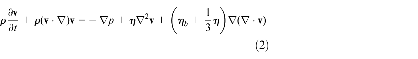
Substituting equations (4a)–(4c) into the governing equations, we can then arrange each term of the equations into the first-order, second-order, and higher-order small components. By retaining only the first-order components on both sides of the equations, we can derive the equations for the first-order pressure and velocity. 15
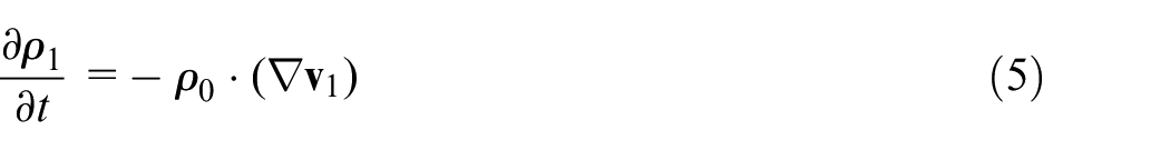
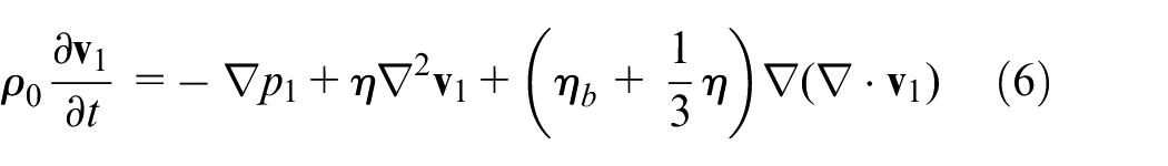
The second-order terms contain higher-frequency oscillations and non-zero mean components. By retaining only the second-order perturbation terms of the Navier-Stokes and continuity equations and then taking the time average, the second-order equations can be derived 15 :

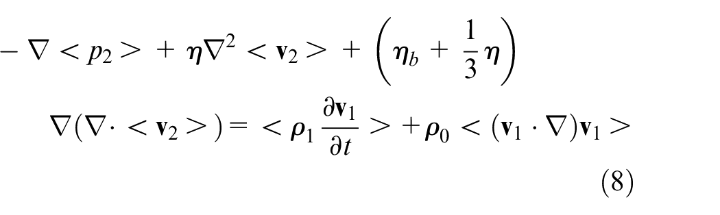
where the point bracket represents the time average.
Time-averaged forces on suspended microparticles
Typical microfluidic experiments use polystyrene particles. We assume these particles are sparse and thus ignore the disturbance made to the flow by the existence of particles. The particle-particle interactions are not considered either. These microparticles are neutrally buoyant, so their movement in the fluid are subject to the ARF and SDF. The ARF (
The ARF on a single suspend particle can be calculated from the first-order solutions to the Navier-Stokes equations. Considering that the particle radius
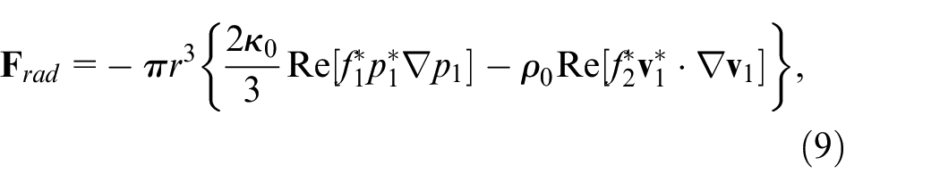
where
where
where
The time-averaged drag force

The SDF increases linearly with the particle size, as seen in equation (15), while the ARF increases with the particle size cubed, as seen in equation (9). Hence, once the particle size exceeds the threshold value, the ARF quickly becomes dominant with a further increase in the particle size. Conversely, for particles smaller than the threshold value, the ARF rapidly tends to zero with a further decrease of the particle size and then the particles’ motion is exclusively governed by the SDF. The motion of the solid particles is governed by Newton’s second law of motion 6 :
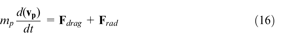
where,
Boundary conditions
The first-order equations (5) and (6) and second-order equations (7) and (8) allow us to numerically solve the pressure field and velocity field in the microfluidic channel to the second order approximation, but the solution has to be accompanied by appropriate boundary conditions. The time-averaged non-zero deformation at the channel boundary is generally in the sub-nanometer scale. Therefore, it is reasonable to ignore the time-averaged deformation of the channel boundaries. In calculating the time-averaged second-order flow field, all the walls correspond to no-slip boundary conditions.
7
The boundary conditions for the first-order acoustic response are more complicated and are the focus of the remaining of this section. The impedance boundary condition (
The impedance boundary condition can be expressed to be 11 :
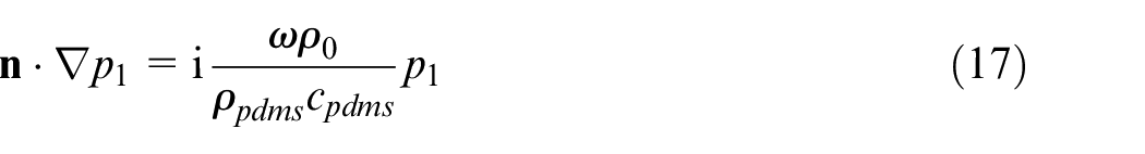
where
Rayleigh waves are the main type of waves produced by the SAW generator. The wave propagates along the y-axis and decays exponentially, which penetrates through the microchannel wall to actuate the fluid inside. Under the acoustic actuation of a single wave, the displacement function at the substrate boundary is 11 :
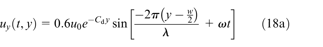
where


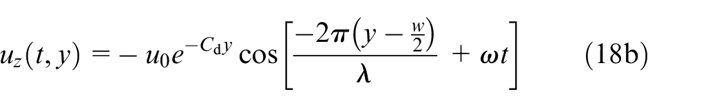
We can then obtain the substrate velocity by taking the partial derivative of the displacement function with respect to time to impose over
Numerical model
Model setup
Acoustophoresis chips are often manufactured by bonding the PDMS channel onto a piezoelectric substrate.
2
The PDMS material is a silicon-based polymer and consists of Sylgard-184-silicone elastomer base and Sylgard-184-silicone elastomer curing agent at a mixing ratio of 10:1 by weight.
16
The material properties of this PDMS (10:1) have been specified in our numerical simulations. The piezoelectric substrate is composed of Lithium Niobate (
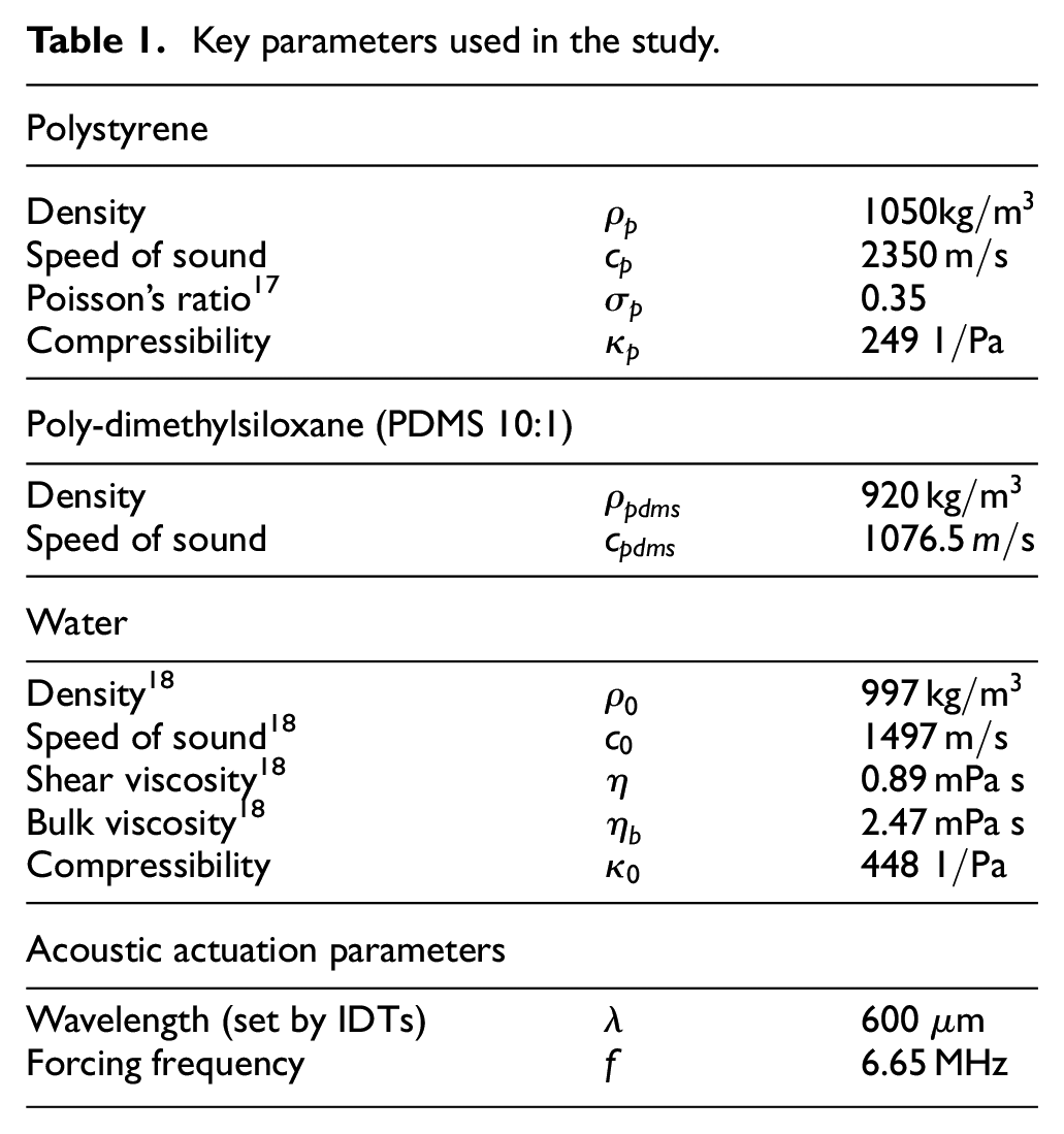
Key parameters used in the study.
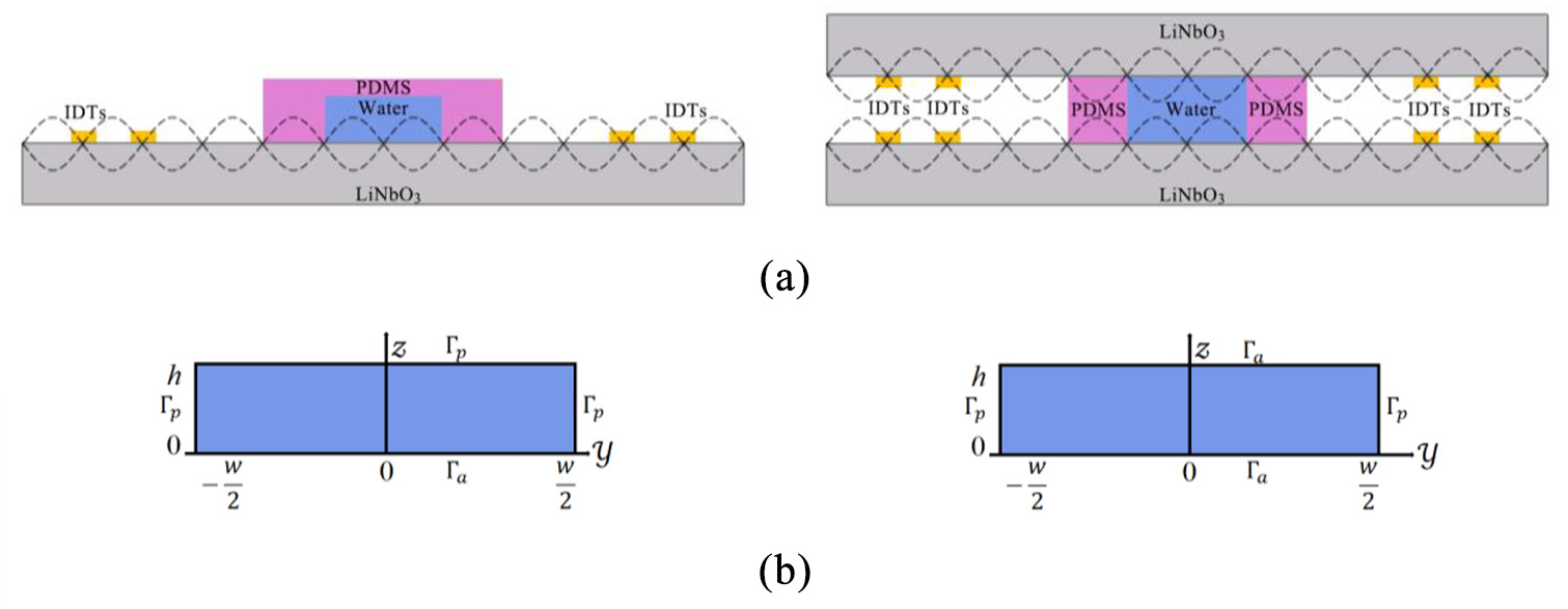
Cross-sectional view of the Model-P (left) and Model-W (right) configurations: (a) positions of the Lithium Niobate substrate and water-filled PDMS channel and (b) locations of the impedance boundary (
Numerical procedure
The governing equations are numerically solved according to the following procedure in COMSOL Multiphysics 5.4. First of all, the first-order acoustic field is obtained by solving equations (5) and (6). Then, the second-order acoustic field is acquired by solving equations (7) and (8). Finally, by combining information from the first-order and second-order fields, we estimate the forces on and trajectories of particles in the microfluid channel.
Mesh convergence analysis
We use triangular mesh for spatial discretization of the computational domain. The mesh convergence analysis is needed to find the suitable mesh resolution. Therefore, we continually reduce element size to decide the threshold at which the result becomes unaffected by further decreasing of the minimum element length
The mesh convergence function
where
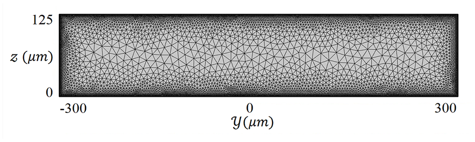
Typical computational mesh with element size
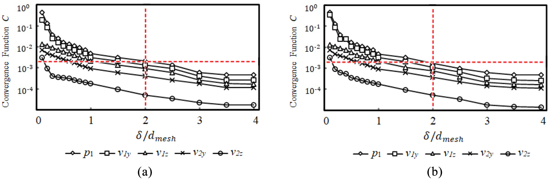
Variations of the mesh convergence functions
Model verification
In the first verification case, we set up the model to be exactly the same as that reported in Nama et al.
11
The polystyrene microparticles are suspended in a water-filled PDMS channel (Model-P). Figure 4(a) demonstrates the comparison of the first-order pressure distribution. An apparent standing wave pattern is formed along the y-axis. The upwards-pointing magenta arrows indicate wave radiation from the bottom wall to the top wall. The first order pressure oscillates with a maximum amplitude of 12.9 kPa according to both studies. Figure 4(b) compares the first-order acoustic velocity distribution (
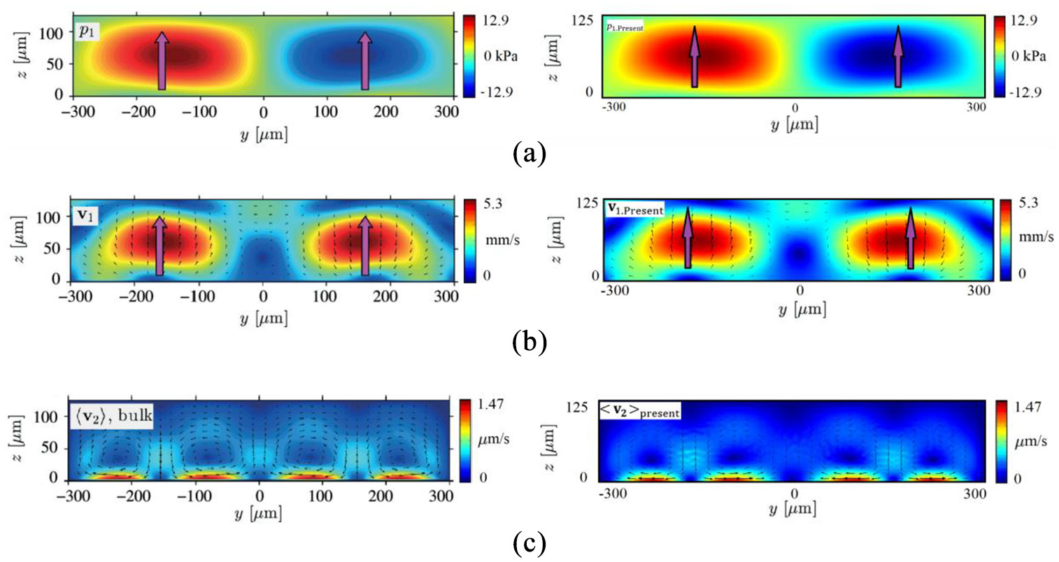
Comparison between the present results (right) and those in Nama et al. 11 (left): (a) first-order pressure field, (b) first-order velocity field, and (c) time-averaged second-order velocity field.
In the second verification case, we set up the model to be exactly the same as that reported in Sun et al.
14
The
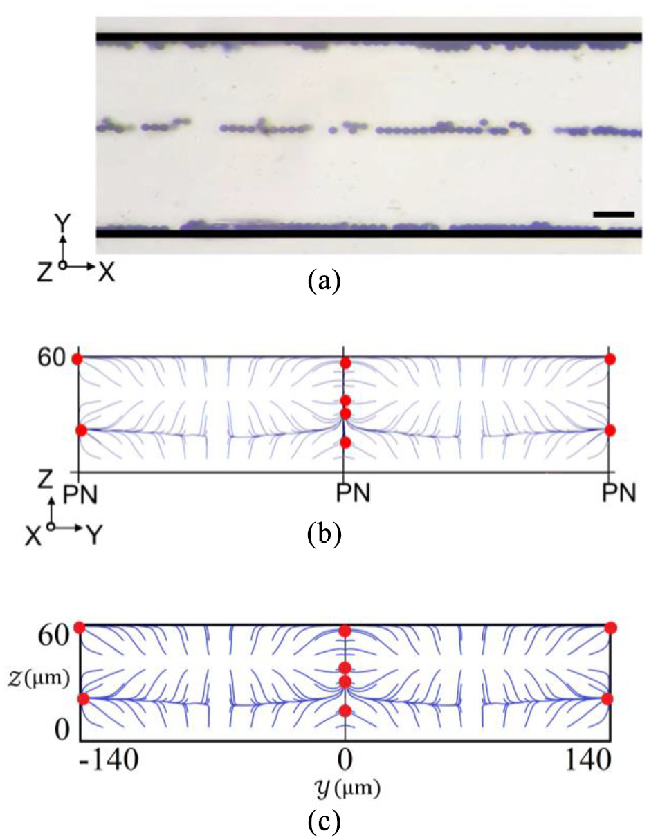
Comparison between the present and Sun et al. 14 : (a) plan view of particles’ trajectories in experiments of Sun et al., 14 (b) cross-sectional view of particles’ trajectories and final positions in simulation of Sun et al., 14 and (c) cross-sectional view of particles’ trajectories and final positions in present simulation.
In our subsequent study, the channel dimensions and acoustic wave properties are taken to be the same as those used in Nama et al. 11 In a separate research by the authors, we varied the channel dimensions and showed that the flow fields over adjacent half wavelength distances in the transverse direction (y-direction) demonstrate an antisymmetric relationship, as can also been seen in Figure 4. In the vertical direction (z-direction), the flow field roughly repeat itself for every wavelength of the acoustic propagation in liquid. Hence, we can easily infer the flow fields and the particle trajectories in microchannels of other dimensions and with acoustic waves of different frequencies. The flow field and particle motion also positively correlate with the amplitude of the acoustic waves specified at the boundary and the correlation is roughly linear.
Comparison between Model-P andModel-W configurations
Flow field
In the conventional Model-P setup, acoustic waves are introduced into the fluid from the bottom wall only. As seen in Figure 4(a), this setup results in the maximum amplitude of the first-order pressure oscillation of 12.9 kPa. The imposed standing wave has three pressure nodes at the bottom surface, located by the sidewalls and in the middle. The acoustic pressure induced by the bottom excitation attains the maximum amplitude some distance above the two antinodes at the bottom surface. In the Model-W setup, the acoustic waves are introduced from both the bottom and top walls to the fluid. As expected, Figure 6(a) shows a significant increase in pressure strength, with the maximum amplitude of the first-order pressure amplitude increased to 228 kPa. In the Model-W setup, the pressure distribution is antisymmetric about the horizontal line through z = 62.5
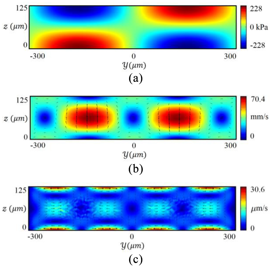
Flow field in a Model-W setup: (a) first-order pressure field, (b) first-order velocity field, and (c) time-averaged second-order velocity field.
Figure 4(c) shows that there are four streaming eddies over the channel width in the Model-P setup. The streaming flow is mirror-symmetric about the vertical line through y = 0, thus two eddies are clockwise and the other two are anti-clockwise. The time-averaged second-order velocity has the maximum magnitude of 1.47
Hydrodynamic forces on particles
The ARF and SDF acting on a solid particle can be calculated once the first-order flow field and the time-averaged second-order flow field have been determined. Their magnitude depends on the particle size. In this section, we consider the situation when the particles are stationary with a radius of
Figure 7(a) shows that the maximum value of the acoustic radiation force is
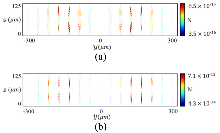
ARF distribution in the y-z plane,
Because we assume that particles’ velocity is zero to demonstrate the forces on them, the direction of the SDF remains the same as that of the time-averaged second-order velocity. As seen in Figure 8, the maximum SDF values for the Model-P and Model-W setups are
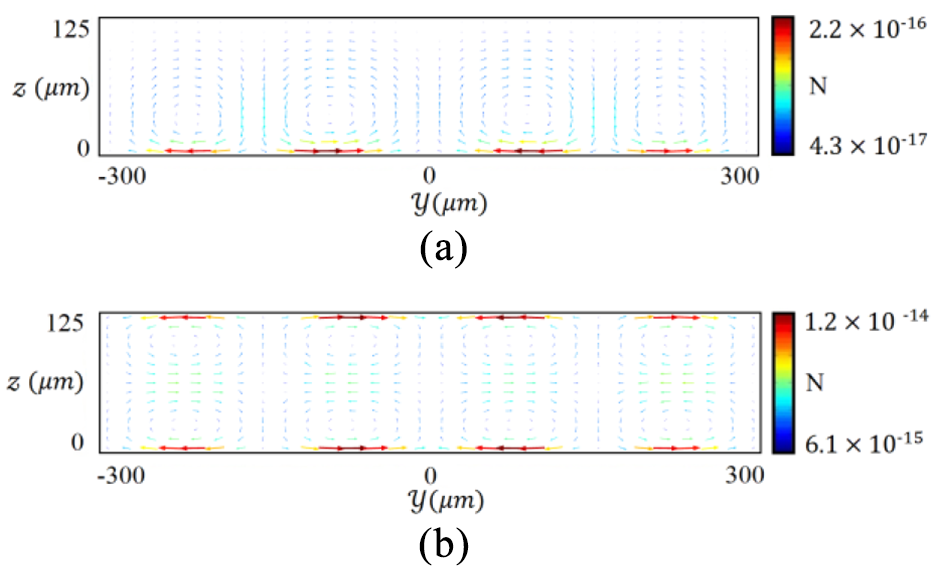
SDF distribution in the y-z plane,
Microparticle trajectories
Knowing the forces acting on the microparticles suspended in the water-filled microchannel, we can plot the particle trajectories using the particle tracing module. For the time-domain simulations, we select the generalized alpha solver in COMSOL, setting the alpha parameter to be 0.5 and specifying a fixed time step Δt = 0.01 s. As can be seen in Figure 9, particles are uniformly distributed over the cross-section in the y-z plane at time zero. In Figure 10, every line represents the trajectory made by a single particle, whereas the color of the line indicates the instantaneous particle velocities. In our study, we assume that the acoustic waves propagate perpendicular to the sidewalls of the microchannel. Hence, the acoustic perturbation is normal to the main flow in x direction, which is the reason for the two-dimensional cross-sectional simulation of the problem in the y-z plane. In the longitudinal direction, that is, x direction, the flow is nearly uniform and the suspended microparticles can be assumed to have the same velocity as the fluid. We neglect the acoustic influence on the movement of the fluid and particles in the longitudinal direction. The three-dimensional motion of a microparticle can be inferred from the particle’s two-dimensional trajectory in the y-z plane. Along the x direction, the particle’s velocity can be estimated to be the liquid flowrate divided by the cross-sectional area of the microchannel, while the particle’s displacement is equal to the product of the velocity and time. Hence, the particle follows a 3-D spiral trajectory to reach its equilibrium position and then maintains a straight trajectory further downstream.
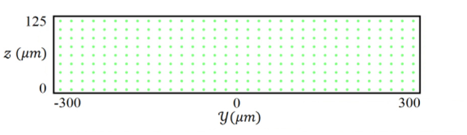
Initial positions of the 297 particles over the cross-section.
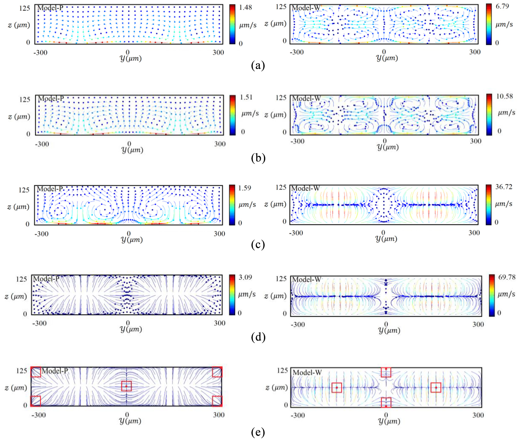
Comparison of the particle in the y-z plane between Model-P and Model-W: (a)
For small particles in the test (r = 0.5 μm and r = 1 μm), as can be seen in Figure 10(a) and (b), both the ARF and SDF acting on the particles are the small, and the SDF arising from the acoustic streaming is the dominant force to determine the particles’ motion. Hence, the particles’ motion is slow and the particles follow the circulation eddies whose characteristics are visualized in Figures 4(c) and 6(c). Corresponding to the stronger streaming flow, the particles’ motion in the Model-W setup is more apparent, as seen in the right graphs in Figure 10(a) and (b). However, the SDF drives particles to loop around streaming vortices rather than concentrate at certain locations. In the Model-P setup, the particles’ displacements is hardly noticeable in 25 s, except in the region very close to the bottom surface.
For the intermediate particle size (r = 2 μm), as seen in Figure 10(c), only the Model-W setup can lead to the gradual concentration of particles in certain regions. In the Model-P setup, the ARF and SDF have similar magnitude and their relative strength varies from region to region. In the upper part of the channel, the ARF is stronger, so particles demonstrate a tendency to slowly move toward the top surface. In the lower part of the channel, the SDF is stronger, so there is no sign of particle concentration. Instead, the large SDF near the bottom is responsible for the circulation of particles inside streaming eddies.
For the larger particles, Figure 10(d) shows a clear trend of particle concentration driven by the dominant ARF in the channel in both setups. In the Model-P setup, particles are pushed toward the middle and four corners of the microchannel. In the Model-W setup, particles are pushed to the middle and the mid-height region in the channel. The final locations where particles will come to rely on the time averaged ARF field. Figure 10(e) highlights the final locations of the particles with red boxes under sufficient duration of the standing SAW exposure. These final locations are the same for all particle sizes larger than the threshold value, but the time required for particles to move to these locations depends on the particle size, which will be discussed in the next section.
Time scale of particle motion
In practical applications, it is extremely important to know the time required for particles to move to their designated positions, as this time determines the minimum length of the channel for successfully microparticle manipulation. Because of the greater magnitude of the ARF acting on large particles, large particles reach their designated positions in shorter time than small particles. To facilitate analyses, we set a target box centered at each of the final positions, as displayed in Figure 10(e). When a particle has moved into a target box, then it is regarded to have arrived at its designated position. The side length of the target box is varied from 30 to 90
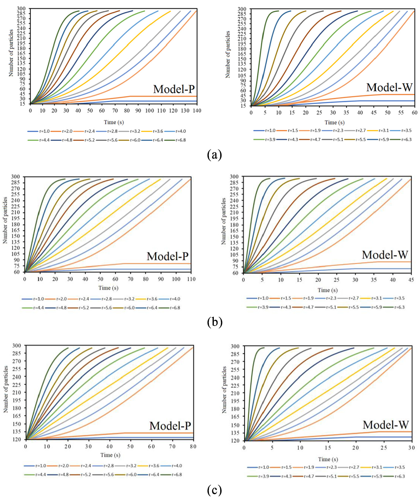
Variation of the number of particles arriving at designated positions with SAW exposure time and its sensitivity to particle radius, SAW excitation method, and target size: (a) side length of target box 30
Our study shows that the critical particle radius is about 2.4 and 1.9
Figure 12 quantitatively shows how the time, required for complete particle concentration, varies with the particle radius, target size, and model setup. The most important finding is that the Model-W setup outperforms the traditional Model-P setup by slightly reducing the threshold particle radius for effective separation and significantly shortening the time scale of the transient process.
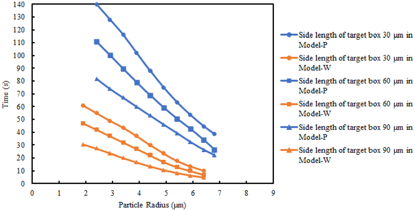
Variations of the minimum required SAW exposure time with particle radius, SAW excitation method, and target size.
Conclusions
In this paper, we examine the detailed flow and hydrodynamic force fields in acoustophoretic channels, including the first-order acoustic pressure (
Footnotes
Declaration of conflicting interests
The author(s) declared no potential conflicts of interest with respect to the research, authorship, and/or publication of this article.
Funding
The author(s) disclosed receipt of the following financial support for the research, authorship, and/or publication of this article: The work has been supported by the National Key Research and Development Program of China under grant no. 2016YFC0402605, the Cambridge Tier-2 system operated by the University of Cambridge Research Computing Service (![]() ) funded by EPSRC Tier-2 capital grant EP/P020259/1 and China Scholarship Council (CSC).
) funded by EPSRC Tier-2 capital grant EP/P020259/1 and China Scholarship Council (CSC).