
Abstract
The reservoir-wave model assumes that the measured arterial pressure is made of two components: reservoir and excess. The effect of the reservoir volume should be excluded to quantify the effects of forward and backward traveling waves on blood pressure. Whilst the validity of the reservoir-wave concept is still debated, there is no consensus on the best fitting method for the calculation of the reservoir pressure waveform. Therefore, the aim of this parametric study is to examine the effects of varying the fitting technique on the calculation of reservoir and excess components of pressure and velocity waveforms. Common carotid pressure and flow velocity were measured using applanation tonometry and doppler ultrasound, respectively, in 1037 healthy humans collected randomly from the Asklepios population, aged 35 to 55 years old. Different fitting techniques to the diastolic decay of the measured arterial pressure were used to determine the asymptotic pressure decay, which in turn was used to determine the reservoir pressure waveform. The corresponding wave speed was determined using the PU-loop method, and wave intensity parameters were calculated and compared. Different fitting methods resulted in significant changes in the shape of the reservoir pressure waveform; however, its peak and time integral remained constant in this study. Although peak and integral of excess pressure, velocity components and wave intensity changed significantly with changing the diastolic decay fitting method, wave speed was not substantially modified. We conclude that wave speed, peak reservoir pressure and its time integral are independent of the diastolic pressure decay fitting techniques examined in this study. Therefore, these parameters are considered more reliable diagnostic indicators than excess pressure and velocity which are more sensitive to fitting techniques.
Keywords
Introduction
Arterial blood pressure waveform, which is affected by many physiological and pathological factors, changes its morphology as it travels along the arterial tree. The mechanical properties of the vessels contribute to these changes; for example, the arterial elasticity reduces the pressure pulsation along the systemic tree. Waves originated by the contracting heart travel forward toward the peripheral arteries, reflect at sites of mismatched impedance (where the arteries, for example, bifurcate or taper) and travel backward toward the heart. The interaction between the forward- and backward traveling waves further induce changes to the magnitude and shape of the pressure waveform. Modeling the pressure waveform is therefore a complex task and different models have been proposed, 1 such as 0D (Windkessel), 1D, and 3D.
In the context of analyzing the pressure waveform, the reservoir-wave approach assumes that the measured arterial pressure can be divided into two components: the reservoir pressure (
The reservoir-wave model was first applied in canine aorta,
2
considering the reasonable assumption that the blood flow is null in diastole. Consequently, it was applied for the calculation of venous reservoir
4
and to any arbitrary arterial location.5,6 However, the calculation of
Specifically, Wang et al.
2
fitted the diastolic decay over the last two thirds of the measured pressure, considering that waves are minimal during this period. The parameters
It is hypothesized that varying the fitting method would significantly change
Materials and methods
Study group
The Asklepios Study is a longitudinal population study focusing on the interaction between ageing, cardiovascular hemodynamics, and inflammation in preclinical cardiovascular disease. 10 A subset comprising 1037 subjects of the total cohort (2524 participants, 1301 women, spanning 4 half-decades: 35–55 years-old) provided data for this study.
Subjects of the Asklepios population were free from manifest cardiovascular disease at study initiation, randomly sampled from the twinned Belgian communities of Erpe–Mere and Nieuwerkerken. All examinations were single-observer, single-device, single-site, and were performed in a single 2-year consecutive timeframe. 10 The procedure included measurements of basic clinical data, blood samples examination, echocardiographic examination, vascular echographic, and tonometric measurements. The study protocol was approved by the ethics committee of Ghent University Hospital and all subjects gave a written informed consent.
Table 1 summarizes the physiological and hemodynamic characteristics of the study group.
Basic characteristics of the study group (n = 1037).
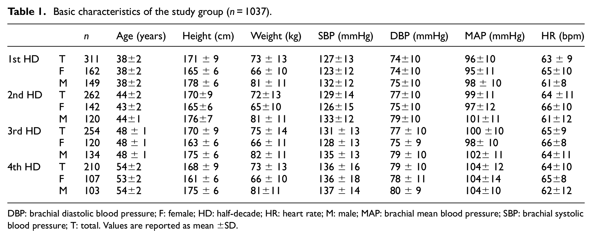
DBP: brachial diastolic blood pressure; F: female; HD: half-decade; HR: heart rate; M: male; MAP: brachial mean blood pressure; SBP: brachial systolic blood pressure; T: total. Values are reported as mean
Hemodynamic measurements
Details of the protocol can be found in Rietzschel et al.
10
Briefly, blood pressure and flow velocity measurements were acquired via applanation tonometry and vascular echography, respectively. The measurements were not simultaneously taken, but acquired during the same vascular examination. The signals were post-processed and subsequently aligned using the algorithm proposed by Swalen and Khir.
11
The tonometric procedure, carried out with a Millar pentype tonometer (SPT 301, Millar Instruments, Houston, Texas, USA), consisted of the following two steps
12
: (1) tracings were collected from the brachial artery for 20 s, at a sampling rate of 200 Hz, then divided into individual beats, using the foot of the wave as fiducial marker, and ensemble-averaged. The averaged tracing was calibrated against oscillometrically measured brachial systolic and diastolic (DBPb) pressure and mean arterial brachial pressure (MAPb) was calculated by numerically averaging the curve; and (2) tonometry was performed on the carotid artery as described in the previous step and tracings were ensemble-averaged and calibrated against the previously calculated tonometric brachial pressure, assuming that diastolic and mean pressure values are fairly constant in large arteries. A scaled carotid pressure waveform (
A commercially available ultrasound system (VIVID 7, GE Vingmed Ultrasound, Horten, Norway), equipped with a linear vascular transducer (12 L, 10 MHz), was used for the scans. Blood flow velocity was measured via Pulsed Wave Doppler with sweep speed equal to 100 mm/s and 5 to 30 ECG-gated cardiac cycles were recorded during normal breathing. The DICOM images were subsequently processed
13
with custom written programs in Matlab (The MathWorks, Natick, Massachusetts, USA). The velocity profile was obtained by averaging the maximum and minimum velocity envelopes and it was finally divided into individual cardiac cycles that were successively ensemble-averaged to obtain a single velocity contour (
Data analysis
Data analysis was performed via custom-made algorithms in Matlab. The algorithm decomposed
where

where
Subsequently, the parameter
The complete reservoir waveform could be obtained via equation (1) and the excess pressure was determined as the difference between the measured pressure
Fitting algorithm settings
The fitting parameters
Properties of the analyses performed.
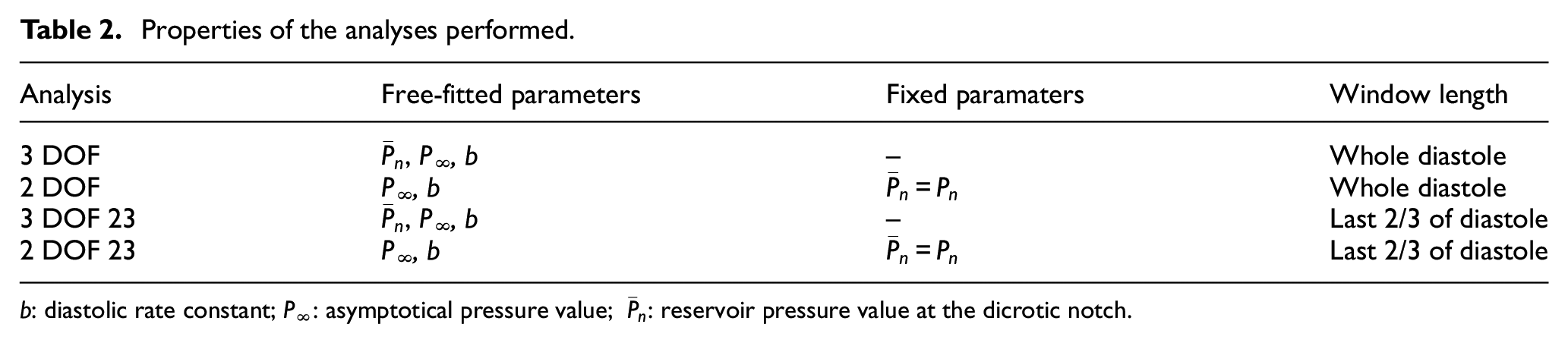
b: diastolic rate constant; P∞: asymptotical pressure value;
The 3 DOF and 3 DOF 23 analyses were characterized by 3 degrees of freedom, because
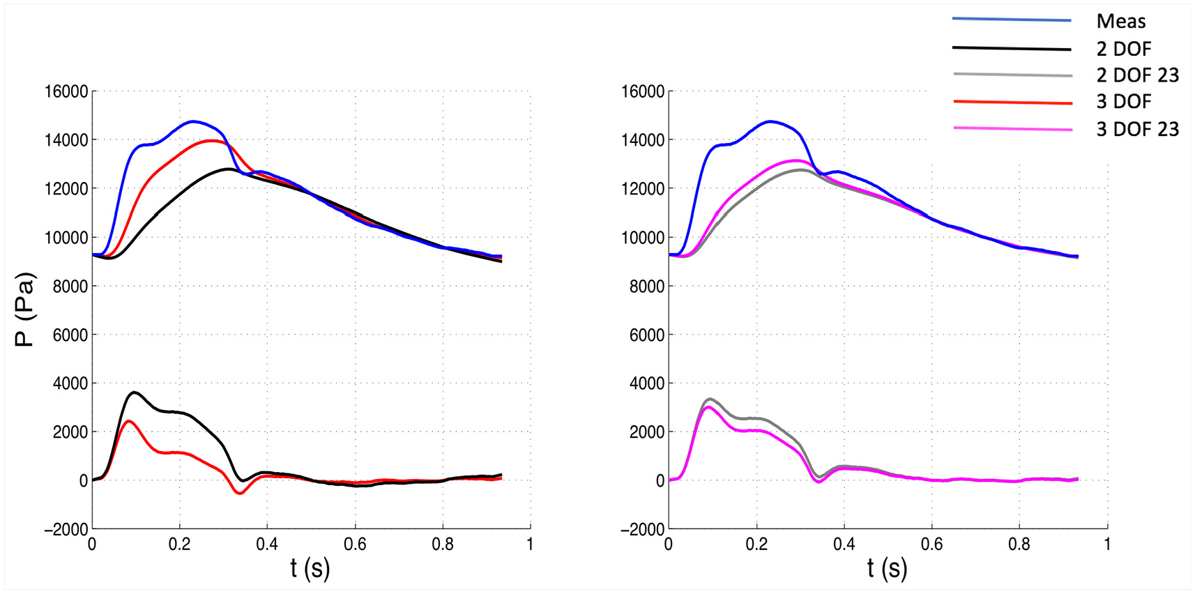
Comparison of pressure waveforms between 3 DOF and 2 DOF settings, whole window (Left) and between 3 DOF and 2 DOF, 23 window (Right) for one patient. The measured pressure is depicted in blue. The top waveforms depicted along with the measured pressure represent the reservoir components, whereas the bottom waveforms the excess components. Meas: measured waveform.
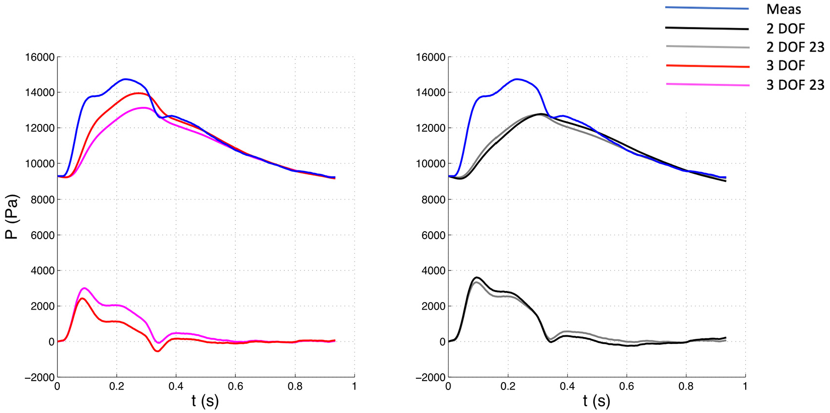
Comparison of pressure waveforms between whole and 23 window with 3 DOF (Left) and 2 DOF (Right) settings for one patient. The measured pressure is depicted in blue. The top waveforms depicted along with the measured pressure represent the reservoir components, whereas the bottom waveforms the excess components. Meas: measured waveform.
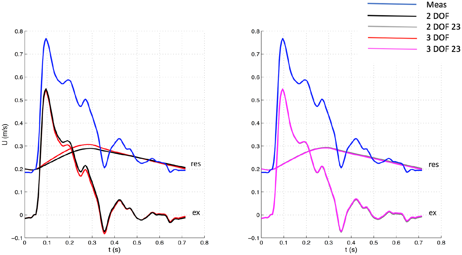
Comparison of velocity waveforms between 3 DOF and 2 DOF settings, whole window (Left) and between 3 DOF and 2 DOF, 23 window (Right) for one patient. The measured velocity is depicted in blue. The top waveforms (“res”) depicted along with the measured velocity represent the reservoir components, whereas the bottom waveforms (“ex”) the excess components. Meas: measured waveform.
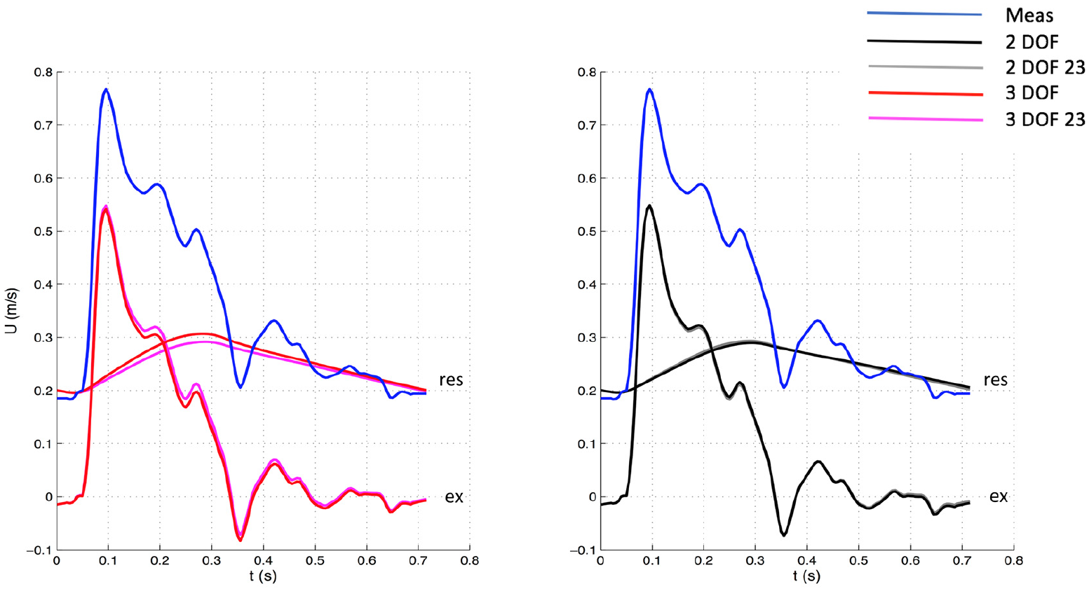
Comparison of velocity waveforms between whole and 23 window with 3 DOF (Left) and 2 DOF (Right) settings for one patient. The measured velocity is depicted in blue. The top waveforms (“res”) depicted along with the measured velocity represent the reservoir components, whereas the bottom waveforms (“ex”) the excess components. Meas: measured waveform.
The fitting algorithms were implemented using the lsqcurvefit function, a Matlab solver optimized for non-linear least squares problems.
The following hemodynamic parameters were calculated: the maxima of
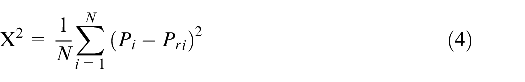
Where N is the number of data points in diastole.
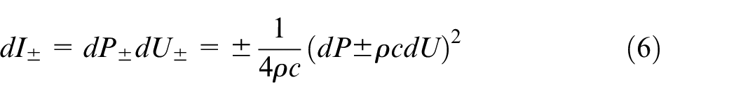
Wave intensity analysis
Wave intensity analysis was performed on both measured waveforms (
Assuming that only forward-traveling waves are present during the early systolic portion of each cardiac cycle, 14 the slopes of the linear part of the PU- and PexUex-loops were used to calculate the corresponding wave speed values [m/s] using the following equation:
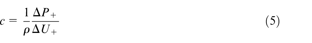
over the early systolic part of the loops (Figure 5). The numerator and denominator in equation (5) refer to the time of the cardiac cycle when waves are running only in the forward direction and the relationship between the measured P and U waveforms is linear for the PU-loop and for the excess waveforms of PexUex-loop. Blood density
After the calculation of wave speed and wave intensity, relevant wave intensity parameters were extracted. The area of the forward compression wave (FCW), which is generated by the contraction of the left ventricle, was derived by integrating the early-systolic peak observed in
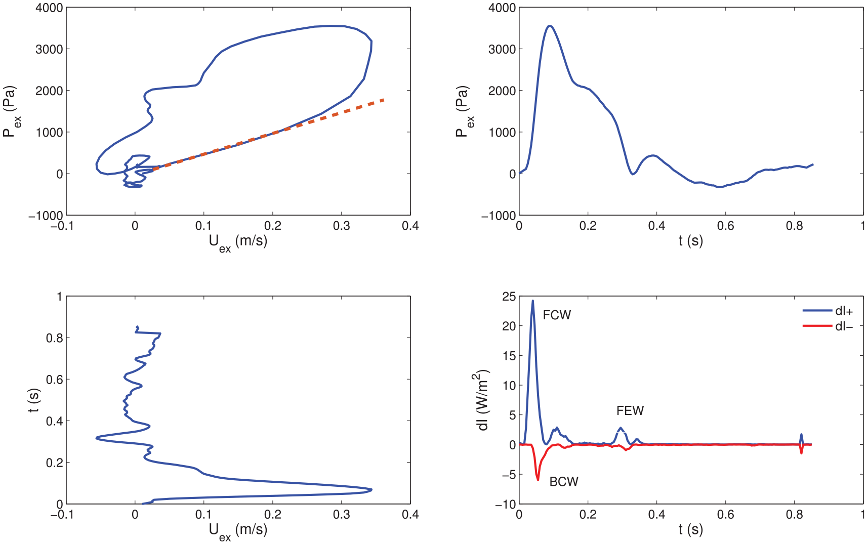
Example of PexUex loop (Top Left), Pex contour (Top Right), Uex contour (Bottom Left) and corresponding wave intensity (Bottom Right; obtained via equation (6)) for one patient. A straight line highlighting the slope of the linear portion is superimposed on the PexUex loop (see equation (5)). Forward compression (FCW), backward compression (BCW) and forward expansion (FEW) waves are labelled in the wave intensity plot. dI+: forward wave intensity component, dI−: backward wave intensity component.
Statistical analysis
All values are reported as mean ± SD, relative to the whole cohort, in the text, tables, and figures. The statistical analysis was performed using SPSS Statistics (version 20, IBM, Armonk, New York, USA). Hemodynamic and wave intensity parameters were statistically compared via one-way analysis of variance (ANOVA) and Tukey’s post-hoc test. A paired two-tailed t-test was also performed for the comparison between PU-derived- and PexUex-derived parameters. Statistical significance was assumed if adjusted p-value<0.05.
Results
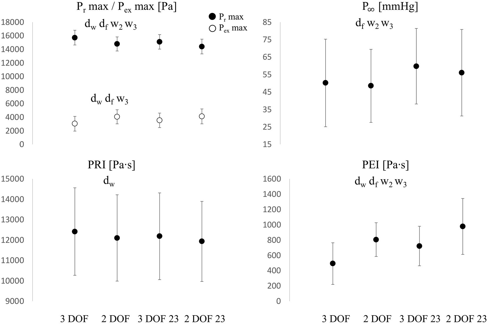
Comparisons of
The diastolic constant
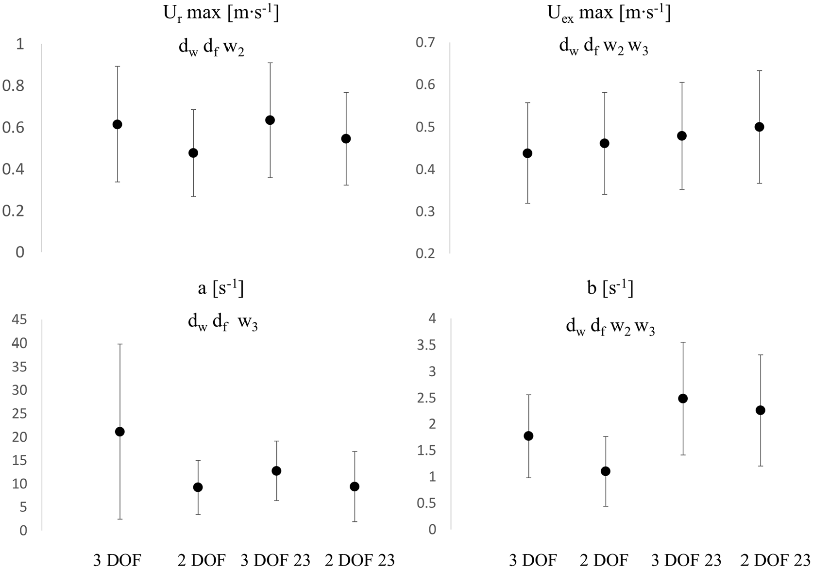
Comparisons of
The error
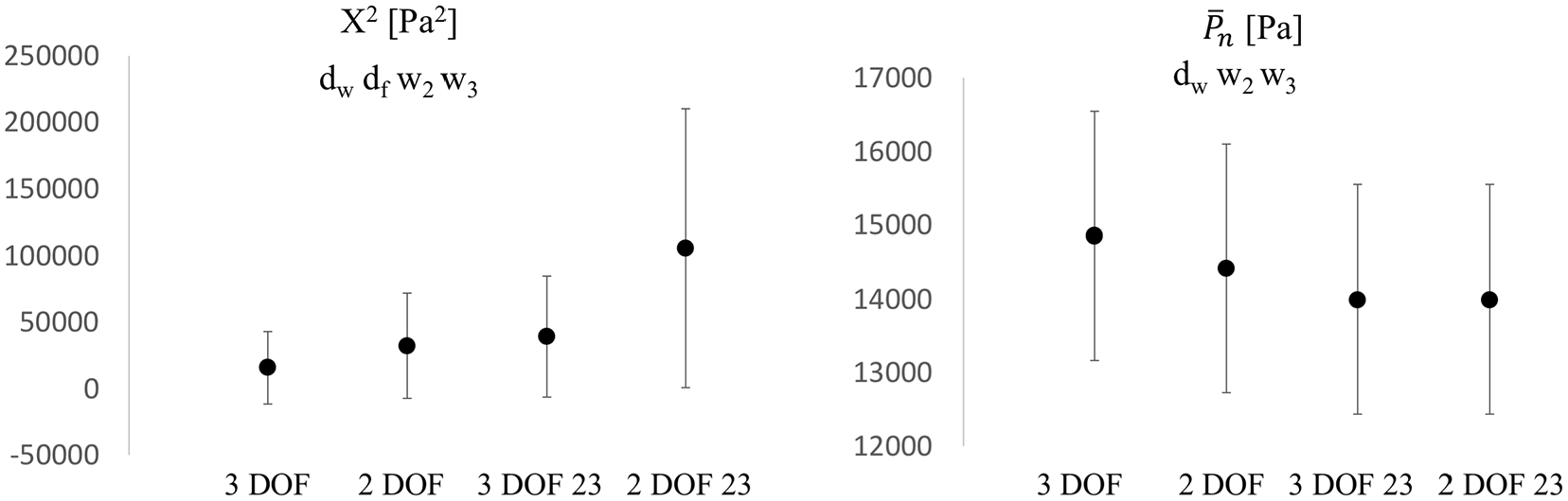
Comparisons of
In the context of wave speed and wave intensity analysis (calculated from Pex and Uex), wave speed (Figure 9) significantly increased (+7%, p < 0.05) from 3 DOF to 2 DOF for the whole window setting and remained fairly unchanged (−1%, p > 0.05) with 23 window. Also, it increased (+8%, p < 0.05) in 3 DOF and remained unchanged (−1%, p > 0.05) in 2 DOF, from whole to 23 window. Overall, wave speed values did not substantially change in-between settings.
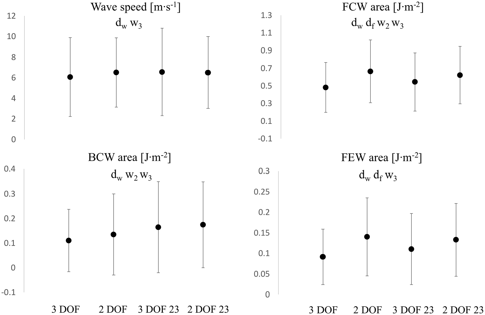
Comparisons of wave speed (Top Left),
FCW area (Figure 9) significantly increased from 3 DOF to 2 DOF, in both window settings: +38% with the whole window and +14% with 23 window. The change exhibited from the whole to 23 window was +13% (p < 0.05) for 3 DOF and −6% (p < 0.05) for 2 DOF. A very similar pattern was recorded for the forward expansion wave. FEW area (Figure 9) significantly increased from 3 DOF to 2 DOF, in both window settings: +53% for the whole window and +20% for 23 window. The change exhibited from whole to 23 window was +21% (p < 0.05) for 3 DOF and −5% (p > 0.05) for 2 DOF. BCW area (Figure 9) increased from 3 DOF to 2 DOF in both window settings: +22% (p < 0.05) and +6% (p > 0.05) for whole and 23 window, respectively. The variation exhibited with change in window (from whole to 23) was significant: +49% (p < 0.05) and +29% (p < 0.05) for 3 DOF and 2 DOF, respectively.
PU-derived parameters were always greater than corresponding PexUex-derived parameters: the biggest difference was recorded with 3 DOF whole window setting (between +19.5% for wave speed and +89.5% for BCW area). Table 3 reports the percentage variations that PU-derived parameters exhibited with respect to corresponding PexUex-derived parameters.
Comparison of PU-derived and PexUex-derived wave intensity parameters.
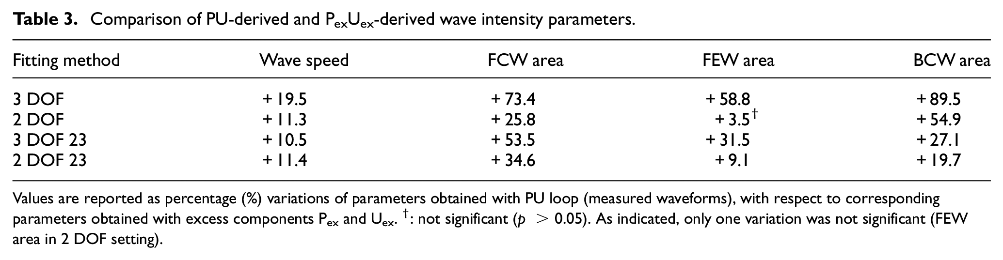
Values are reported as percentage (%) variations of parameters obtained with PU loop (measured waveforms), with respect to corresponding parameters obtained with excess components Pex and Uex. †: not significant (p > 0.05). As indicated, only one variation was not significant (FEW area in 2 DOF setting).
Discussion
This parametric study aimed to compare various common carotid hemodynamic and wave intensity parameters, using different fitting techniques for the calculation of the reservoir pressure and velocity waveforms, assuming the reservoir-wave hypothesis (with a single exponential decay) for the decomposition of the arterial pressure.
Whilst
In general, the variation of fitting methods brought substantial modifications to the calculated waveforms, mainly highlighted by
The 23 window ensures an almost perfect match between measured pressure and reservoir waveform in the last two thirds of diastole, but leaves a bigger “gap” in the first diastolic third (Figure 1), compared to the whole window. The differences in gaps are more visible in Figure 2 (3 DOF 23 vs 3 DOF reservoir contour). The gap is associated with a slightly positive excess pressure waveform in the first diastolic third and may be related to the presence of little wave activity in the beginning of diastole.
The changes in the shape of both reservoir and excess waveforms affected hemodynamic and wave intensity parameters. Fixing the dicrotic notch (2 DOF setting,
Variations did not occur independently, as can be easily seen by re-arranging equation (2):
where
The significant variations in hemodynamic parameters caused by changes in fitting techniques had effects on wave intensity, resulting in substantial differences in all main parameters. However, wave speed values did not substantially change with fitting methods, suggesting that it seems insensitive to those. As can be seen in Figures 1–4, excess pressure and velocity waveforms tended to preserve the slope of the upstroke, being also similar to that of corresponding measured waveforms. Table 3 shows that wave speed, being measured with both PU loop and
The age of patients used for this study spans across two decades and the data show a broad spectrum of basic characteristics (Table 1). Therefore, it is important to higlight the wide variation in each of the parameters under study across the cohort. A couple of selected extreme cases has been reported in Table 4 to demonstrate the range of the results. Further, although another window size is used for the fitting of the reservoir pressure waveform in the literature, namely the last third (1/3) of diastole (as specified in the “Introduction”), it was not considered in this work. It was believed that a further comparison, between 2/3 and 1/3 of diastole, was not necessary at this stage and the difference was not expected to be significant to alter the current data interpretation or conclusions.
Range (variability) demonstration: Two extreme cases of the cohort.
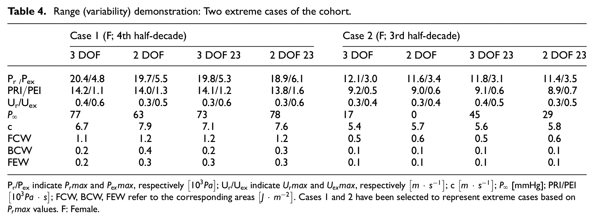
Pr/Pex indicate
In this study,
Finally, whilst we acknowledge that the applicability of the reservoir-wave theory is still a matter of debate,18,19 it is important to consider that the scope of the study, the assessment of sensitivity of the derived parameters to choices made when fitting the reservoir pressure, is parametric in nature. As such this work is a quantitative contribution toward the ongoing discussion pertaining the determination of the asymptotic pressure, which requires fitting the diastolic pressure waveform or part of it.
Limitations
In all of the reservoir-wave earlier work, the diastolic decay was fitted to a single exponential curve and we have recently studied the effect of changing the value of the single asymptotic pressure on the wave intensity parameters. 20 However, fitting an exponential function can be perfomed via a multi-exponential approach, as noted in other areas of physical sciences. In fact, this possibility has been recently demonstrated using physiological data. 18 Notewithstanding, the determination of the parameters pertaining the multi-exponential approach is more complex and cannot be established with a high degree of confidence. 21 Therefore, in the current work we focused on the more common single exponential decay for the reservoir-wave approach.
Pressure and velocity measurements in this study were recorded sequentially and the two waveforms had to be aligned to satisfy conditions of the analysis. However, physiological changes either during or between the recordings were not implicated in this study and given that the time interval between recordings was short, it was safely considered that the hemodynamic parameters did not change significantly between recordings. Therefore, it can be carefully assumed that the sequential recordings of the data did not have negative effects on the analysis, results or conclusions.
Conclusion
This quantitative study of hemodynamic and wave intensity parameters, under different fitting techniques for the reservoir pressure and velocity, demonstrated that the fitting method could bring significant variations in values and trends. Despite the changes in the shape of the
This study showed that reservoir pressure features and wave speed, being less substantially dependent on the fitting technique, could be more reliable diagnostic indicators.
Footnotes
Declaration of conflicting interests
The author(s) declared no potential conflicts of interest with respect to the research, authorship, and/or publication of this article.
Funding
The author(s) received no financial support for the research, authorship, and/or publication of this article.