Study of the influence of multiple factors on the boundary layer of a high-lift LPT with the RBF-GA method

Abstract

In a high-altitude cruising state, boundary layer separation exists in high-lift low-pressure turbines, and inflow conditions corresponding to different blade designs can directly affect the working efficiency of low-pressure turbines. In particular, the reduced frequency of wake and free-stream turbulence intensity in an inlet flow can greatly influence boundary layer separation and transition development. In this paper, the influence of different inflow turbulence intensities and reduced wake frequencies on the development of suction surface boundary layers in high-lift low-pressure turbines under the influence of upstream wakes is studied by numerical simulations and experiments. Due to the combination of inflow free-stream turbulence intensity and reduced wake frequency, many inflow conditions can be chosen in the design process, and the unsteady influence of upstream wakes complicates the boundary layer flow. In this paper, an RBF (radial basis function)-GA (genetic algorithm) machine learning method is used to explore the optimal inlet conditions corresponding to the minimum profile loss of the Pak-B profile. The search region of the free-stream turbulence intensity is 2%–4%, and the reduced frequency of the wake is changed by changing the flow coefficient, whose variation range is 0.7–1.3. It is found that the RBF-GA machine learning method can attain an inflow condition with a lower profile loss while using the same amount of computation and effort.

Overview

Low-pressure turbines are important components that affect the performance and weight of aero-engines. In LEAP and GEnx multistage LPT engines, the weight of high-lift low-pressure turbines accounts for approximately 20%–30% of the engine’s total weight. ¹ Wisler et al. ² noted that when low-pressure turbine efficiency increases by 1%, engine fuel consumption decreases by 0.7∼0.9%. Curtis et al. ³ reported that suction surface boundary layer loss accounts for 60% of profile loss, which is important for reducing the loss. Mayle, ⁴ Halstead, ⁵ and Schobeiri ⁶ showed that the main part of a boundary layer comprises laminar flow and that the local adverse pressure gradient allows the boundary layer to easily separate, resulting in a significant decrease in efficiency, especially at high altitudes and low Reynolds numbers. This problem restricts the wide application of high-lift low-pressure turbines.

Scholars have conducted considerable research on constraining suction surface separation in high-lift low-pressure turbines. For example, active blowing devices, ⁷ vibration devices, ⁸ V-shaped grooves, ball sockets, ⁹ mix lines, ¹⁰ and other structures have been designed to augment blades. In recent years, unsteady wakes inherent in turbomachinery have been used to induce the transition of the separation boundary layer in advance and to constrain separation. Xiaodong Ruan et al. ¹¹ showed the wake-inducing transition process of a suction surface boundary layer with experimental and large eddy simulation (LES) results. Benjamin W et al. ¹² used LES to compare two working conditions with or without wake and showed the presence of wake on the boundary layer separation inhibition region. Howell ¹³ noted the feasibility of making use of nonsteadiness, especially using wake to control loss, on high-lift blades and indicated that the wake has a constraining effect on boundary layer separation. The experiments of Hodson and Dawes ¹⁴ indicated that a wake sweep can constrain separation and reduce profile loss. Haselbach ¹⁵ of Rolls-Royce successfully applied this technology to reduce the weight of low-pressure turbines in civil aero-engines by 38%.

After determining the usefulness of wakes, scholars began to extensively examine the control effect of wakes on the boundary layer. Volino ¹⁶ found that when the reduced frequency increases as the flow coefficient decreases, boundary layer separation between wakes disappears, indicating that increasing the reduced frequency helps to constrain separation. The study also indicated that increasing the free-stream turbulence intensity constrains separation but is not as helpful as increasing the reduced frequency. Schobeiri ⁶ concluded that the reduced frequency does not significantly affect the initiation and reattachment position of the separation bubble but that increasing the reduced frequency reduces the maximum thickness of the separation bubble. Mahallati and Sjolander ¹⁷ studied several working conditions, including different turbulence intensities, flow coefficients, and reduced frequencies of incoming flow. Their results showed that increasing the reduced frequency constrains separation, but the profile loss first decreases and then increases with increasing reduced frequency, and the influence of the free-stream turbulence intensity of incoming flow is obvious only at a low reduced frequency. Coull ¹⁸ noted that the total profile loss under the wake effect is the result of a balance between the separation loss generated by the separation bubble and the loss in the turbulent region under the influence of inlet parameters such as the Reynolds number, free-stream turbulence intensity, and reduced frequency.

In the above studies, the isometric cross-traversal method was used over a range of parameter changes to study multiple working conditions and compare them with each other. This method is more suitable for mechanistic research. CFD optimization design aided by machine learning has been developed in recent years, showing a good application effect. Shinkyu J et al. ¹⁹ combined a Kriging model with a GA to design a lift–drag ratio and showed that it can effectively reduce the design time compared with a simple CFD design. Ney R S et al. ²⁰ used an artificial neural network to optimize aircraft design. Liming Chen et al. ²¹ used a gradient-modified Kriging model to optimize airfoil design. M. Mohammadi et al. ²² used an ANN (artificial neural network)-GA method to optimize rotor parameters.

In the present paper, the RBF method is used as a surrogate model to estimate the profile loss of low-pressure turbines. The RBF surrogate model, as a robust and accurate interpolation method, is suitable for fitting functions with a high nonlinear degree and is widely used in research on fluids and other fields.^23–30 In this study, the RBF and GA are combined to supplement CFD; the reduced frequency and free-stream turbulence intensity are taken as variables, the profile loss coefficient is taken as the objective function for optimization, and the experimental results are used for verification. This approach overcomes the poor engineering applicability caused by optimizing a single inlet parameter in previous studies or the lack of a globally optimal parameter due to partial traversal optimization. Moreover, we verify that the genetic algorithm-like machine learning method can accelerate the design progress and reduce the consumption of CFD and experimental resources in the preliminary design. In this paper, the traditional traversal method is also used to determine an optimal strategy experiment, which is compared with the RBF-GA method and verified by experiments.

Optimization processes and machine learning methods

Optimization process

The RBF-GA machine learning optimization process adopted in this paper is shown in Figure 1. First, a method similar to an orthogonal experiment is used to select the conditions, and the basic database is obtained by experiment and simulation. The RBF is deployed to the database to acquire the surrogate model. The global lowest point is obtained by the genetic algorithm based on the RBF surrogate model. Then, experiments and simulations are used to verify the prediction point and obtain data. If the current cycle number (N) is greater than the set cycle number (N_set) or the difference between the estimated value and the verified value ( $\left|\mathrm{\Delta }{\mathrm{Y}}_{\mathrm{m}}\right|$ ) is less than 0.001, this point constitutes the optimization result; otherwise, the validation data are input into the database and the process continues.

Figure 1.

Optimized process deployment.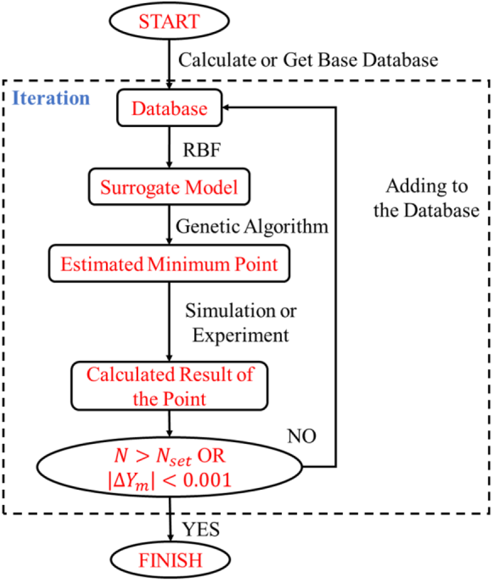

To verify the advantages of this RBF-GA method, the traditional traversal method, which has the same computational consumption, is used for comparison. Both the RBF-GA method and the traditional traversal method have a 13-point basic orthogonal database. In the traditional traversal method, another 12 points are added to the database. The final version contains 25 uniform test points, presented as a 5*5 square for selecting the best one. As shown in Figure 2, the flow coefficient and free-stream turbulence intensity within the selected range are divided by 5 grid points, and all crossing conditions are tested. In the RBF-GA method, the cycle number is set to 12. Therefore, a total of 25 test points are also considered in the RBF-GA method.

Figure 2.

Traversal test points (the abscissa is the FSTI, and the ordinate is the flow coefficient).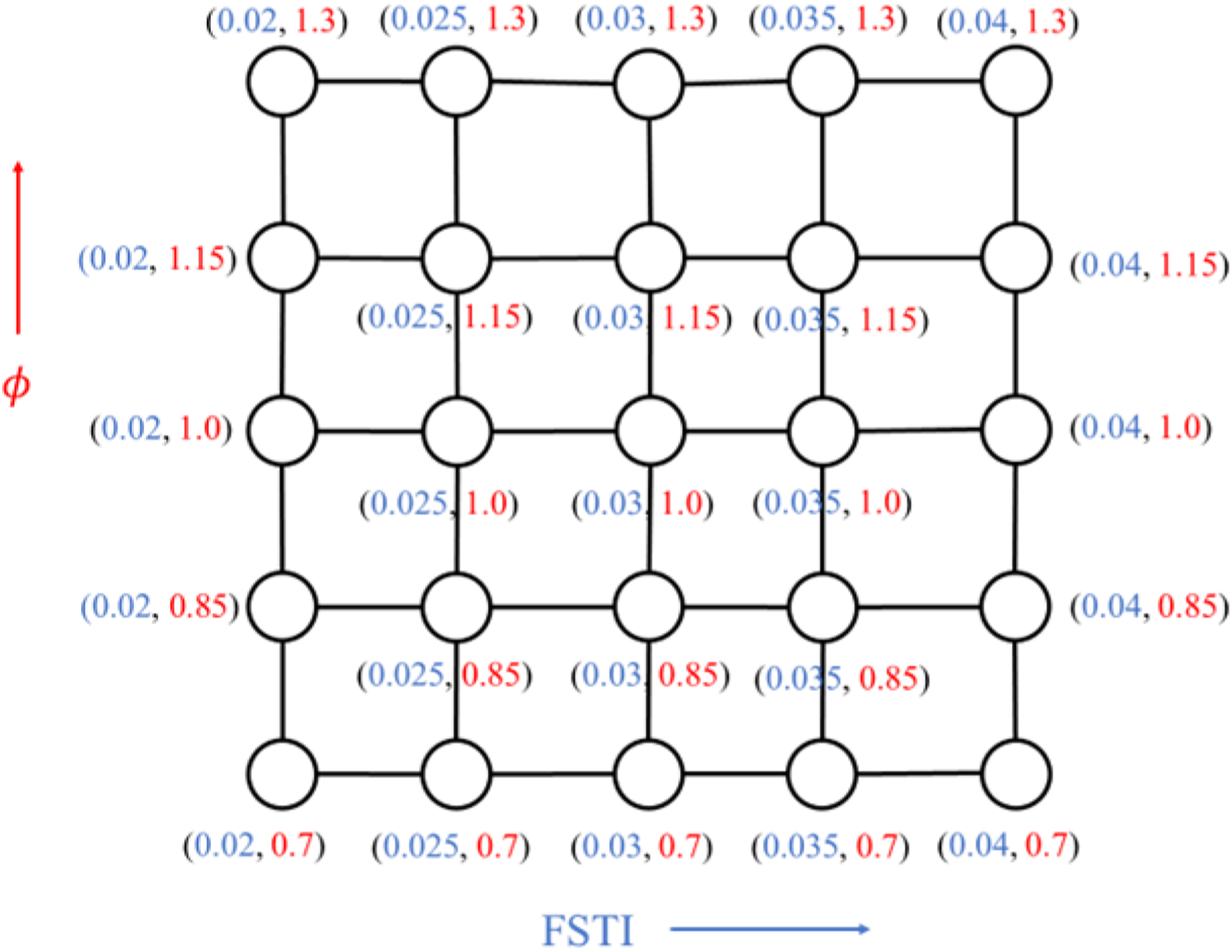

In this study, the cascade parameters are not changed, and the reduced frequency is inversely proportional to the flow coefficient. The input parameters selected for optimization are the flow coefficient and the free-stream turbulence intensity, and the output parameters are the profile loss coefficient. Before the optimization, a large range of turbulence of 0.001–0.2 and flow coefficients of 0.5–2.0 were tested in advance. Finally, the range where the best inflow condition is most likely to occur is selected: a turbulence of 0.02–0.04 and a flow coefficient of 0.7–1.3.

Brief description of the RBF

As mentioned above, the RBF is a widely used alternative model^23–30 with a specific concept similar to minimizing the total surface curvature of a fitted surface passing through sample value points. Combining the RBF with machine learning can be used to predict the extreme value of a reduced-order model.

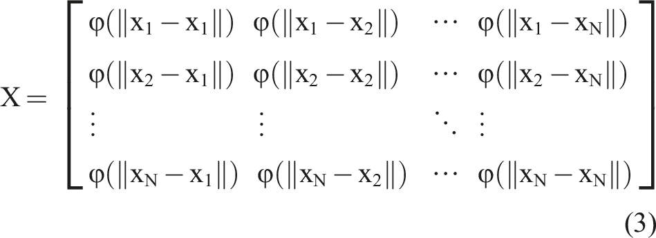
The basic RBF replacement model S(x) is shown in equation (1)

$\mathrm{S}\left(\mathrm{x}\right)=\sum {\mathrm{\beta }}_{\mathrm{i}}\mathrm{\phi }\left(\Vert \mathrm{x}-{\mathrm{x}}_{\mathrm{i}}\Vert \right)$

(1)

where i = 1,2,3..., N; N is the number of data points, ${\mathrm{\beta }}_{\mathrm{i}}$ is the coefficient to be solved, $\mathrm{\phi }\left(\right)$ is the radial basis function, that is, the RBF kernel, and $\Vert \mathrm{x}-{\mathrm{x}}_{\mathrm{i}}\Vert$ is the Euclidean space distance between two points. There are many common RBF kernel functions; the one used in this article is the inverse multiquadric kernel.

By substituting the data points $\left({\mathrm{x}}_{\mathrm{i}},{\mathrm{y}}_{\mathrm{i}}\right)$ into equation (1) and considering $\mathrm{S}\left({\mathrm{x}}_{\mathrm{i}}\right)$ as ${\mathrm{y}}_{\mathrm{i}}$ , an equation of n–n unknown terms can be obtained. The solution of ${\mathrm{\beta }}_{\mathrm{i}}$ can be obtained, which can be expressed by the matrix in equation (2)

$\left[{\mathrm{\beta }}_1{\mathrm{\beta }}_2\cdots {\mathrm{\beta }}_{\mathrm{N}}\right]={\mathrm{X}}^{-1}\left[{\mathrm{y}}_1{\mathrm{y}}_2\cdots {\mathrm{y}}_{\mathrm{N}}\right]$

(2)

where X is defined as in equation (3)

$\mathrm{X}=\left[\begin{array}{ll}\begin{array}{ll}\mathrm{\phi }\left(\Vert {\mathrm{x}}_1-{\mathrm{x}}_1\Vert \right)& \mathrm{\phi }\left(\Vert {\mathrm{x}}_1-{\mathrm{x}}_2\Vert \right)\\ \mathrm{\phi }\left(\Vert {\mathrm{x}}_2-{\mathrm{x}}_1\Vert \right)& \mathrm{\phi }\left(\Vert {\mathrm{x}}_2-{\mathrm{x}}_2\Vert \right)\end{array}& \begin{array}{ll}\cdots & \mathrm{\phi }\left(\Vert {\mathrm{x}}_1-{\mathrm{x}}_{\mathrm{N}}\Vert \right)\\ \cdots & \mathrm{\phi }\left(\Vert {\mathrm{x}}_2-{\mathrm{x}}_{\mathrm{N}}\Vert \right)\end{array}\\ \begin{array}{ll}⋮& ⋮\\ \mathrm{\phi }\left(\Vert {\mathrm{x}}_{\mathrm{N}}-{\mathrm{x}}_1\Vert \right)& \mathrm{\phi }\left(\Vert {\mathrm{x}}_{\mathrm{N}}-{\mathrm{x}}_2\Vert \right)\end{array}& \begin{array}{ll}\ddots & ⋮\\ \cdots & \mathrm{\phi }\left(\Vert {\mathrm{x}}_{\mathrm{N}}-{\mathrm{x}}_{\mathrm{N}}\Vert \right)\end{array}\end{array}\right]$

(3)

Using the RBF method, surrogate models can be built on the database to predict the better position.

Numerical methods and experimental settings

Simulation setting

In this study, the commercial CFD software ANSYS-CFX15.0 is used to balance the computational load and simulation accuracy, and the LES model and Smagorinsky subgrid model are selected for numerical simulation. The van Driest wall function is used to address the dissipation of turbulent kinetic energy in the near-wall region. The dumping factor and Smagorinsky constant are set as 25 and 0.1, respectively. As shown in previous studies,^31,32 these settings can accurately simulate the unsteady flow of an LPT suction side boundary layer at a low Reynolds number. The central difference method and the second-order accurate backward Euler integral method are used to discretize the spatial derivatives.

The numerical simulation mesh in this study is shown in Figure 3. The domains of the wake bar and the blade are colored blue and red, respectively, in Figure 3. The distance from the trailing edge of the cascade to the outlet is 1.5Cx to prevent wall pressure reflection of the outlet. The distance between the upstream wake bar and the leading edge of the cascade is 0.6Cx. The computational geometry is set according to the experimental bench of the Civil Aviation University of China. Based on the studies of Mittal et al. ³³ and Michelassi et al., ³⁴ the spanwise width of the computing domain is set as 0.2Cx. An O-shaped topology is used in the area around the blade and the bar. An H-shaped topology is used to generate the mesh for the other region of the block. The mesh is densified in the near-wall area of the blade so that the suction surface y⁺ reaches 1 and the maximum pressure surface y⁺ is lower than 5. Finally, after mesh independence verification, as shown in the following text, a 20M mesh is used for simulation. The cascade parameters are shown in Table 1.

Figure 3.

Numerical simulation mesh.

Table 1.

Parameters of the cascade in the experiment.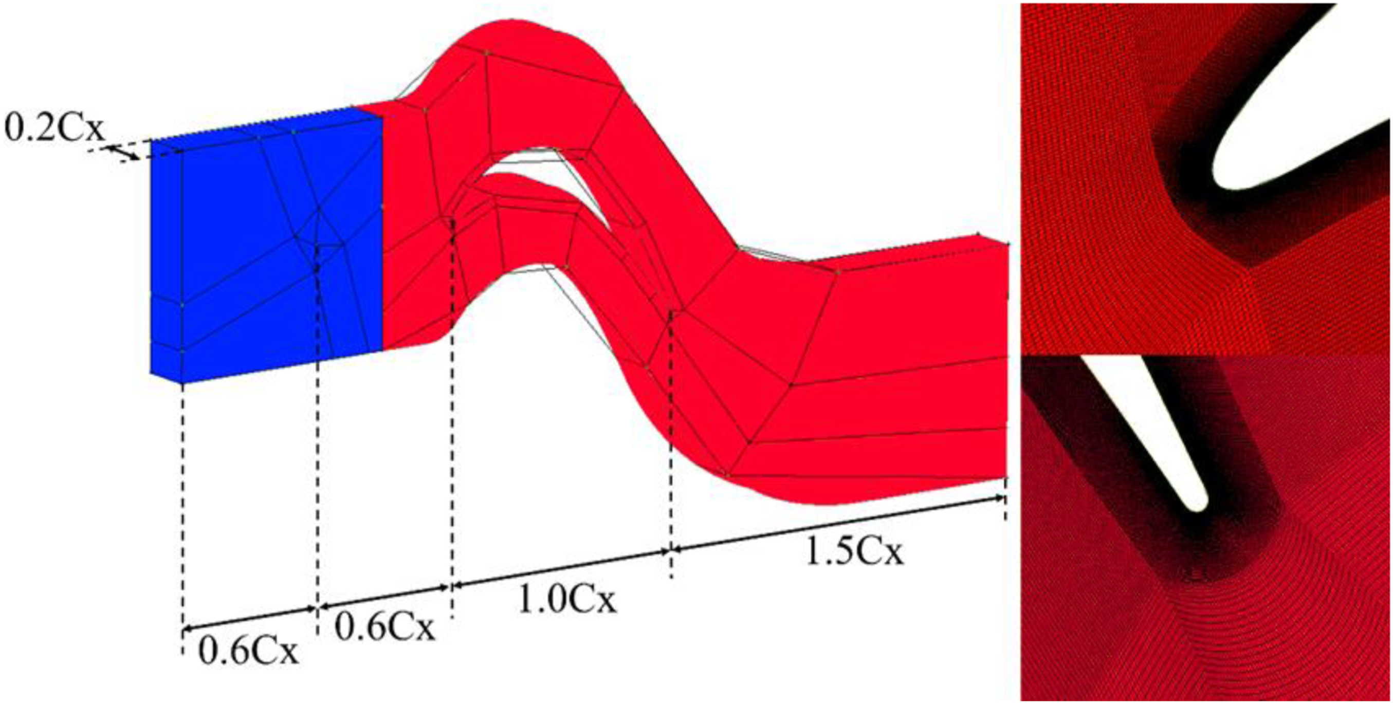

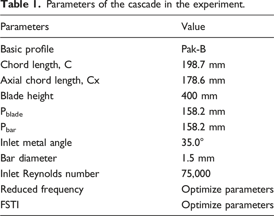
Parameters	Value
Basic profile	Pak-B
Chord length, C	198.7 mm
Axial chord length, Cx	178.6 mm
Blade height	400 mm
Pblade	158.2 mm
Pbar	158.2 mm
Inlet metal angle	35.0°
Bar diameter	1.5 mm
Inlet Reynolds number	75,000
Reduced frequency	Optimize parameters
FSTI	Optimize parameters

The periodic boundary condition is enforced in the pitchwise direction. A no-slip boundary is employed at the blade and wake bar surface. A free-slip boundary is employed in the spanwise direction. The interface between the two blocks is set to a frozen rotor in the steady calculation for the initial value and a transient rotor stator in the unsteady calculation. The inlet condition is set as the velocity inlet, and the outlet condition is set as the pressure outlet. The wake bar movement is simulated by bar block rotation.

In the calculation process, the RANS model is first calculated to obtain the convergence result as the initial value, and then the LES model is used to calculate until the wake of one cycle completely leaves the computational domain. Finally, 2 cycle calculations using the LES model are carried out to obtain data for optimization, and then 9 cycle calculations are finished for flow field analysis. A wake bar passing through a cascade pitch is defined as a cycle. Each cycle contains 2000 steps, making a time step of 2e-5 s. Each step takes 10 iterations, which makes the residual less than 5e-5. The Courant‒Friedrichs‒Lewy (CFL) number is approximately 0.9. The CFL number is large only at the front and back edge of the blade, being approximately 1.8. A workstation is used to perform the RBF-GA process in this study, and each calculation consumes approximately 12.5 days. The traversal method data and initial database are calculated in parallel by using another two workstations. The 9 cycles of data used for flow field analysis consume approximately 52 days.

Experimental facilities

The experiment was carried out on the linear cascade experimental platform of the Civil Aviation University of China, which mainly includes a fan, rectification section, contraction section, diversion section, and cascade installation platform. The measured AVR of the outlet flow from the wind tunnel is 0.97, between 0.97 and 1.02, ³⁵ proving a good two-dimensionality of the cascade. A turbulence grid is installed in front of the cascade to generate turbulence intensity. Figure 4 shows the details of the experiment. The relative motion of a single blade row was simulated by moving cylindrical bars upstream of the stationary cascade. ³⁶ A Scanivalve DSA 3217 pressure sensor is used to test the static pressure distribution on the suction surface (28 test points) and the pressure surface (9 test points). A calibrated seven-hole pressure probe is used to measure the average total pressure and static pressure at the inlet and outlet. The pressure sampling frequency is 100 Hz, and the sampling range is ±2500 Pa. An array of 25 individual surface-mounted hot-film sensors (half of the SenFlex 92,071) is bonded onto the suction surface of the blade. The sensors are equally spaced at an interval of 5.08 mm, covering 48.4%–96% of the airfoil suction surface at mid-span. The hot-film sensors are connected to a Dantec Streamline Pro. An eight-channel PXI-based DAQ A/D is used to collect signals. The uncertainty of the experimental data is estimated according to the measurement uncertainty guidelines. ³⁷ The pressure data from the Scanivalve DSA 3217 have a full-range uncertainty of 0.12%. The uncertainties of velocity and static pressure are estimated to be approximately 1.7% and 3.5%, respectively. The calibration of hot-film sensors is extremely difficult and subject to errors. Uncalibrated sensors have been shown to provide semiquantitative but meaningful information about the states of boundary layers. ³⁵

Figure 4.

(a) Experimental platform of the Civil Aviation University of China. (b) Experimental blade. (c) Hot film.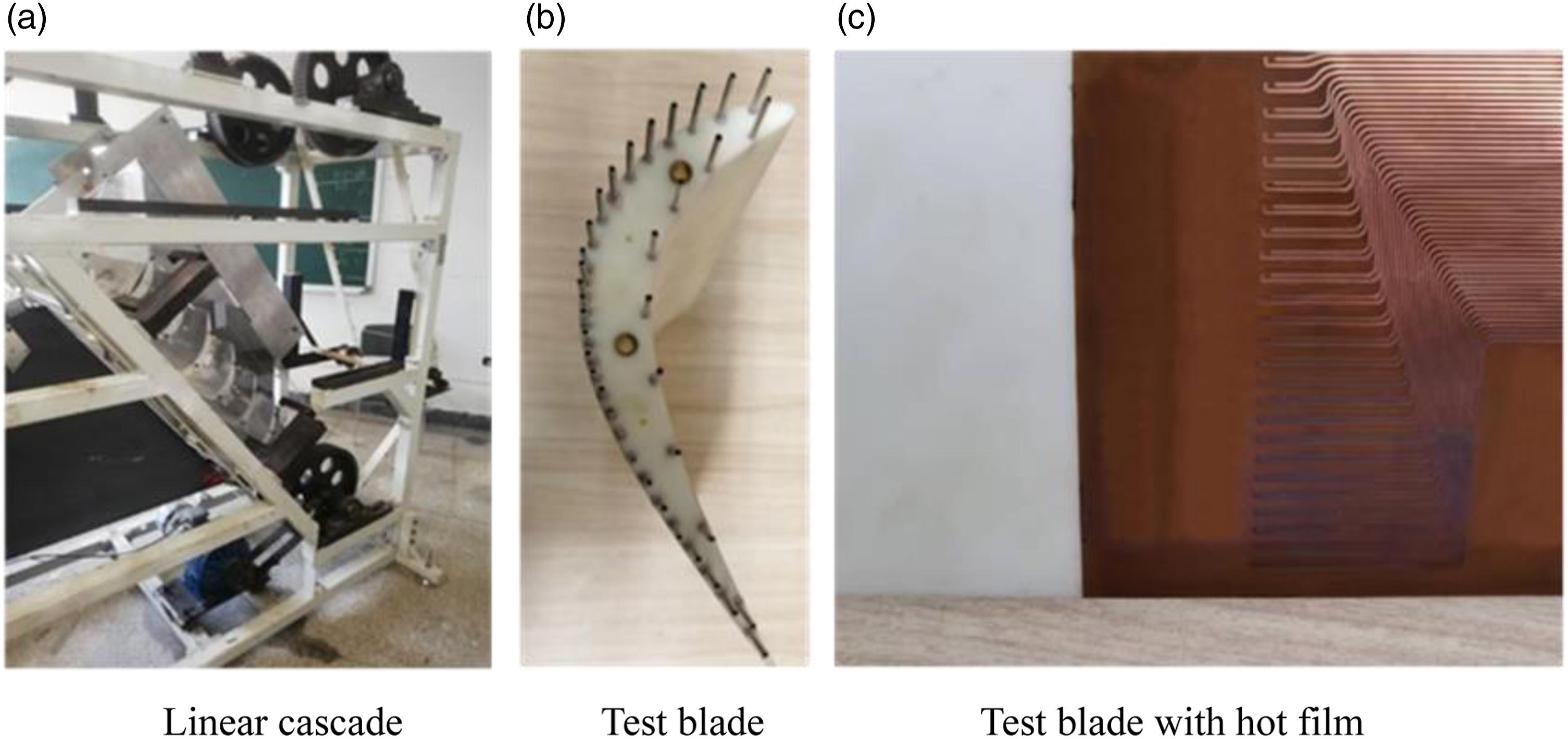

Mesh independence verification

In this study, three kinds of meshes are tested for mesh independence analysis. Figure 5 shows the wall static pressure difference between the 20M mesh, 6M mesh, and 35M mesh under a steady inflow condition. As shown in Figure 5, the difference between the static pressure results of the pressure surface and the suction surface of the 20M mesh and the 35M mesh is small, especially downstream of the axial position s/S₀ = 0.65. Balancing the computation cost and the accuracy, the 20M mesh is selected.

Figure 5.

Mesh independence for Re = 75,000 and FSTI = 2.83%; the ordinate is the absolute value of the pressure difference (unit: Pa). (a) Pressure surface (b) Suction surface.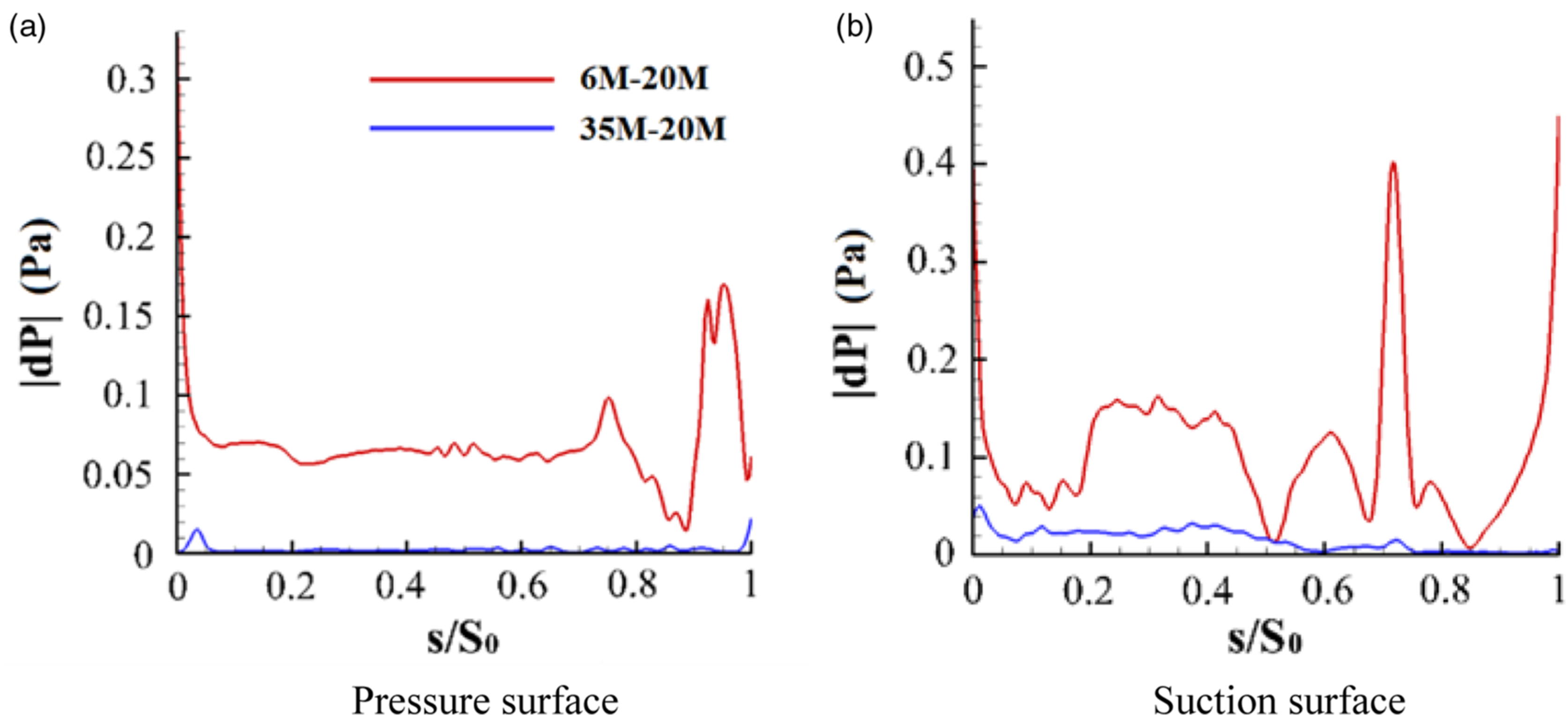

Optimization results and analysis

Optimization results and comparison

Figure 6 shows the normalized data of the profile loss coefficient under all 37 tested conditions. The ordinate is the flow coefficient, and the abscissa is the FSTI. The contour is the normalized total pressure loss coefficient ${\mathrm{Y}}_{\mathrm{p}}^{*}$ , whose calculation method is shown in equation (4), where ${\mathrm{Y}}_{\mathrm{p}}$ is the total pressure loss coefficient and ${\mathrm{Y}}_{\mathrm{p},\max }$ and ${\mathrm{Y}}_{\mathrm{p},\min }$ are the maximum and minimum values of all data, respectively

${\mathrm{Y}}_{\mathrm{p}}^{*}=\frac{{\mathrm{Y}}_{\mathrm{p}}-{\mathrm{Y}}_{\mathrm{p},\min }}{{\mathrm{Y}}_{\mathrm{p},\max }-{\mathrm{Y}}_{\mathrm{p},\min }}$

(4)

Figure 6.

Optimization process.

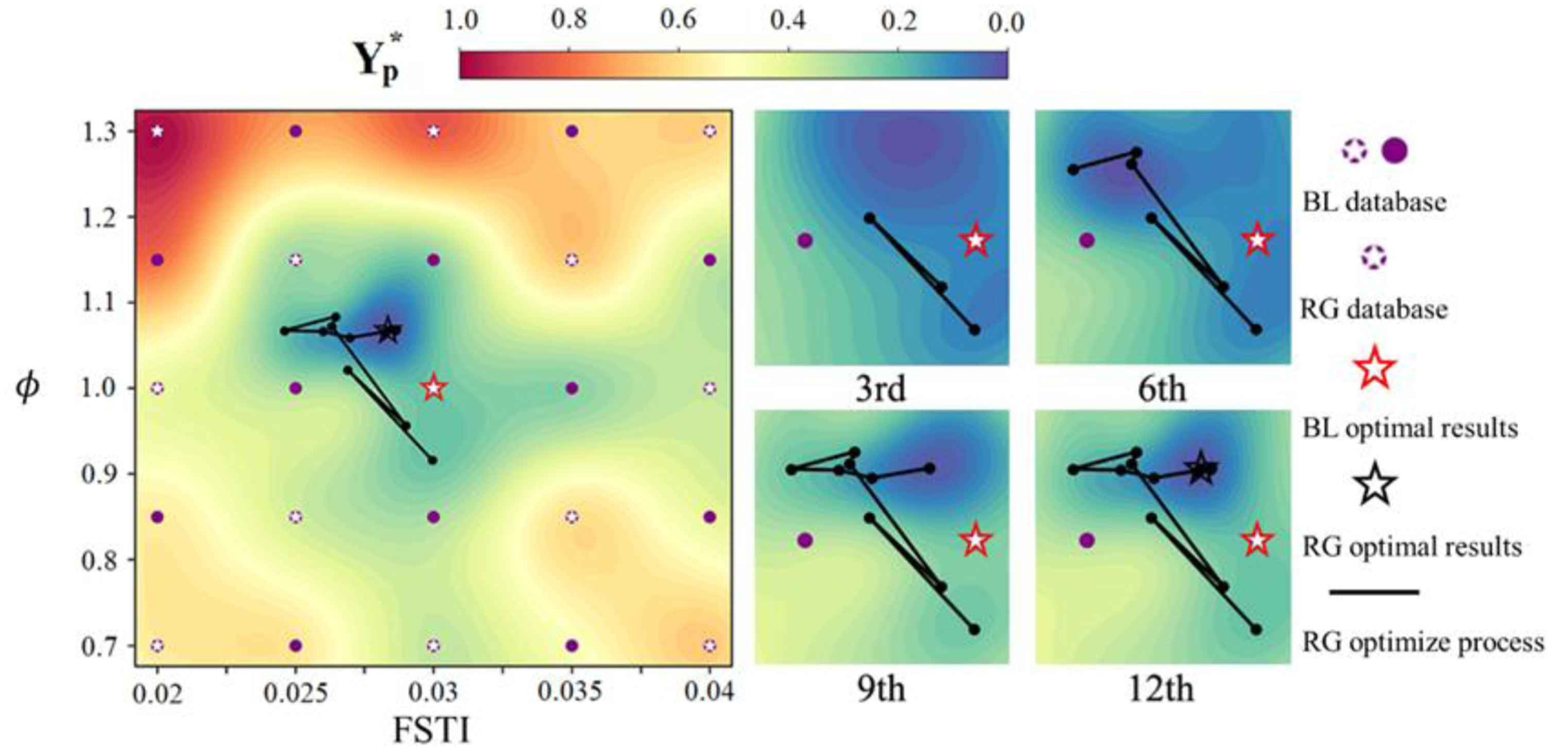
The purple points show the 25 conditions tried in the traversal method. The white star marks the orthogonal design initial database. The lowest ${\mathrm{Y}}_{\mathrm{p}}^{*}$ result of the traversal method, the BL result, with $\text{FSTI}=3\%$ , $\mathrm{\varphi }=1.0$ , $\text{Fr}=1.129$ , and ${\mathrm{Y}}_{\mathrm{p}}^{*}=0.214$ , is selected to be the optimal result of the original basic database, marked by a black star. The variation in the data over the process of the RBF-GA optimization is shown in the right four partial graphs of Figure 6. The black line is linked individually to the estimated minimum condition for each cycle of the optimization. The result of RBF-GA optimization for step 12, the RG result, is marked by a red star with $\text{FSTI}=2.83\%$ , $\mathrm{\varphi }=1.067$ , $\text{Fr}=1.057$ , and ${\mathrm{Y}}_{\mathrm{p}}^{*}=0$ .

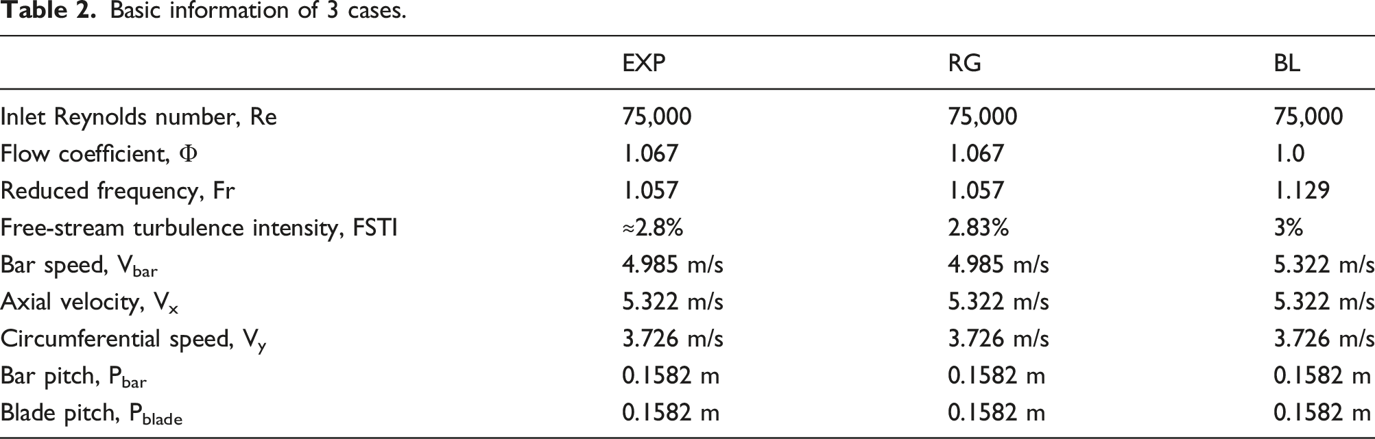
In Figure 6, the inflow conditions of the BL and RG results are similar, with the FSTI having only a 0.17% difference and $\mathrm{\varphi }$ having only a 0.067 difference, which results in a difference of Fr = 0.072. However, the RG method finds a result with ${\mathrm{Y}}_{\mathrm{p}}^{*}$ 0.214 lower, which may be due to some small mechanism or a better fit of the free-stream turbulence intensity and reduced frequency, as analyzed later.

The inflow condition of the BL result (called the BL case) and the inflow condition of the RG result (called the RG case), as well as the experimental condition for RG result verification (called the EXP case), are listed in Table 2. The free-stream turbulence intensity of incoming flow in the RG case is slightly less than that in the BL case, and the flow coefficient is slightly larger than that in the BL case, with reduced frequency showing the opposite trend; the flow coefficient of both is approximately 1.

Table 2.

Basic information of 3 cases.

	EXP	RG	BL
Inlet Reynolds number, Re	75,000	75,000	75,000
Flow coefficient, $\mathrm{\Phi }$	1.067	1.067	1.0
Reduced frequency, Fr	1.057	1.057	1.129
Free-stream turbulence intensity, FSTI	≈2.8%	2.83%	3%
Bar speed, Vbar	4.985 m/s	4.985 m/s	5.322 m/s
Axial velocity, Vx	5.322 m/s	5.322 m/s	5.322 m/s
Circumferential speed, Vy	3.726 m/s	3.726 m/s	3.726 m/s
Bar pitch, Pbar	0.1582 m	0.1582 m	0.1582 m
Blade pitch, Pblade	0.1582 m	0.1582 m	0.1582 m

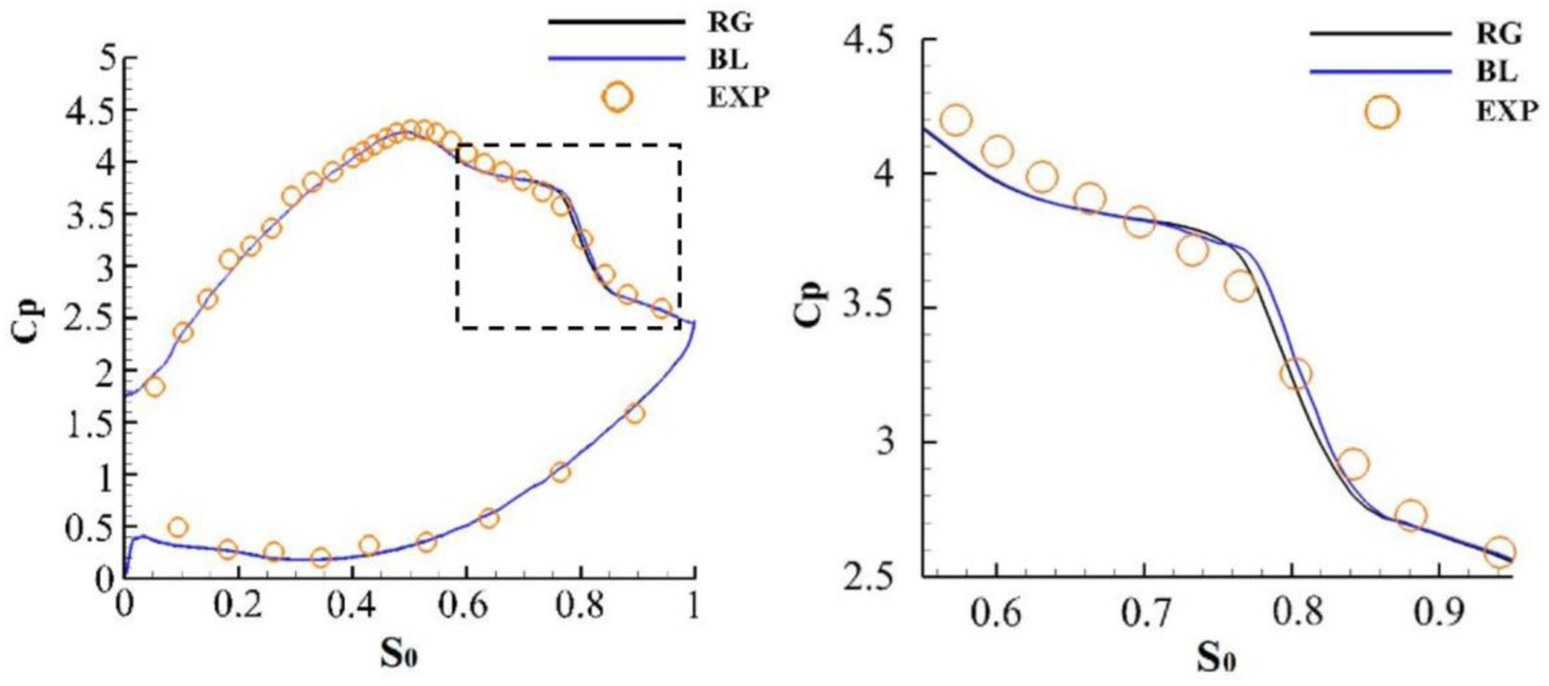
Blade surface static pressure coefficient distribution

Figure 7 shows the static pressure coefficient Cp of the blade surface under the RG, BL, and EXP cases. The abscissa is the normalized arc length on the suction surface; Cp is calculated by equation (5), where ${\mathrm{P}}_{\infty }$ is the inflow total pressure, ${\mathrm{P}}_{\text{local}}$ is the local static pressure of the measuring point, $\mathrm{\rho }$ is the density, and ${\mathrm{U}}_{\text{in}}$ is the inflow velocity

${\mathrm{C}}_{\mathrm{p}}=\frac{{\mathrm{P}}_{\infty }-{\mathrm{P}}_{\text{local}}}{\frac{1}{2}\mathrm{\rho }{\mathrm{U}}_{\text{in}}^2}$

(5)

In Figure 7, the Cp at the aft half of the suction surface shows a platform area, from 0.58S₀ to 0.76S₀ in the RG case, which corresponds well with the experimental results. The BL line and RG line almost coincide at the acceleration zone. The RG line platform area is shorter than the BL line, which indicates that the average separation bubble is slightly smaller under the RG case.

Figure 7.

Static pressure coefficient distribution on the blade surface.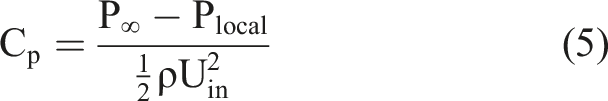

Shape of wake

Figure 8(a) and (b) show the TKE contour and instantaneous perturbation velocity when the wake is about to contact the leading edge of the blade. Figure 8(c) shows the schematic diagram of the wake shape under the RG and BL cases. The wake center (WC) refers to the strong negative jet between the front and rear vortex of the wake. The wake tail (WT) refers to the highly turbulent area where the wake contacts the blade. Under the influence of reduced frequency, the average angle between the wake negative jet strip and blade leading edge (hereafter called the wake angle) in the RG case is smaller than that in the BL case, which causes the wake in the RG case to stretch farther into the passage and brings the RG wake close to the leading edge of the suction surface. Under the influence of turbulence, the BL wake high turbulence region is wider, so the BL wake is close to the blade at the leading edge. The combination of the two effects makes the distance between the wake and the blade surface in the RG and BL cases basically the same, but the wake center in the RG case is closer to the blade and more lordotic over the whole flow.

Figure 8.

Schematic diagram of the wake shape. (a) RG (b) BL (c) Comparison of contours of the wakes.

Instantaneous Q isosurface

Figure 9 shows partial transient flow field diagrams within a period for the RG and BL cases, including a Q diagram of the flow field on the right blade, normal vorticity of the semiboundary layer wall on the left blade, and average TKE contour of the background. The normal vorticity of the wall is also used for staining on the Q surface, and the Q value chosen for the isosurface is 1200,000 s⁻². The Q vortex identification method refers to Ref. [38]. The identification of Klebanoff streaks (KS) is based on the methods used ¹⁸ and Ref. [39]. The head of Klebanoff streak (HKS) is marked as a black line on the left blade and has a speed of 0.88U₀. ¹⁸ The lower left corner of the figure shows the leading edge of the blade, showing the generation process of the KS under the shear sheltering effect. Considering that the inlet mainstream velocity of the two cases is identical, resulting in the same velocity of the wake in the passage, the wake-passing period of the RG case, T_R, is used for normalization in both cases to ensure comparison uniformity. The moment when the wake is about to contact the leading edge of the blade, it is selected as the zero time moment in both cases, which is conducive to the study of KS motion.

Figure 9.

RG and BL CFD results. (a) 0.00T_R-RG, 0.00T_R-BL. (b) 0.10T_R-RG, 0.10T_R-BL. (c) 0.20T_R-RG, 0.20T_R-BL. (d) 0.30T_R-RG, 0.30T_R-BL. (e) 0.40T_R-RG, 0.40T_R-BL. (f) 0.50T_R-RG, 0.50T_R-BL. (g) 0.60T_R-RG, 0.60T_R-BL. (h) 0.64T_R-RG, 0.67T_R-BL.

In Figure 9(a), when t = 0.00T_R, the WT has reached the leading edge of the blade in both cases, the previous WC has left the passage, and the KS is not prominent on the leading edge of the blade. In the downstream region after 0.7S₀, the vortex roll-up from the separation bubble appears distorted and ruptured, showing the characteristics of a natural transition.

In Figure 9(b), at t = 0.10T_R, the WT is cut by the leading edge of the blade in both cases, and KSs are formed due to the “shear sheltering” effect. ⁴⁰ The HKS positions of the two cases are close, reaching 0.06S₀. The wake stretches in the passage, and the wake head reaches the middle part of the passage. Under the RG case, because of the effect of a small wake angle, the wake head moves farther downstream, but the wake does not reach the separation area. The separation area after 0.7S₀ still shows the characteristics of a natural transition.

In Figure 9(c), when t = 0.20T_R, the WT is nearly cut off by the leading edge of the blade in both cases, the KS coverage area magnifies, and the HKS reaches approximately 0.16S₀. At the RG position near 0.25–0.3S₀, the WC amplifies the weak KSs formed by FSTI, which become WCAKSs (wake center amplified Klebanoff streaks) and are delineated with a blue circle. However, the intensity of the WCAKSs is lower than that of the KSs at upstream 0–0.2S₀.

In Figure 9(d), at t = 0.30T_R, the WT in both cases has been cut off by the leading edge of the blade, and strong streaks are no longer generated at the leading edge of the blade. The WCAKS under the RG case is continuously enhanced and moves to 0.54S₀, and its tail has contacted and fused with the KS amplified by the WT. A WCAKS also appears in the BL case, but the intensity is much lower than that in the RG case. Because the WC in the RG case is closer to the suction surface, the WC at 0.74S₀ induces a full-span K-H structure (W1). However, there is no obvious full-span K-H structure in the BL case.

In Figure 9(e), at t = 0.40T_R, the KS amplified by the WT is no longer generated because the WT has left the leading edge. The strength of the WCAKS in the RG case increases and moves to 0.68S₀. The tail of the WCAKS has fused with the KS and becomes a part of the KS. Under the BL case, the WCAKS strength also increases and moves to 0.64S₀. The WC induces a full-span K-H structure (W1) at the 0.74S₀ position. In the RG case, the WC induces W2 after W1.

In Figure 9(f), when t = 0.50T_R, the newly formed W3 K-H structure is impacted and deformed by the WCAKS in the RG case. The W3 K-H structure impacted by streaks cannot be fully formed. The adjacent W2 becomes unstable, and the damaged W2 interacts with W1, accelerating the instability of W1. In the BL case, the WCAKS impacts the W2 K-H structure, and W1 is affected and becomes unstable. Because the WCAKS is weak, the W2 K-H vortex is unstable, and W1 is not affected as much as in RG.

In Figure 9(g), when t = 0.60T_R, W2 in the RG case has been completely disrupted, and W1 has also become completely unstable. In the BL case, the middle part of K-H vortex W2 is impacted by the WCAKS and disconnected. Since W2 blocks most KS impacts, W1 still maintains a full-span structure, which increases the momentum thickness and blade profile loss at the trailing edge. Due to the large number of streaks entering the separation transition zone, the full-span K-H structure does not appear in either case. In the BL case, only small-scale part-span vortex structure W3 appears upstream of W2. In the RG case, only a greatly distorted vortex structure W4 appears.

Figure 9(h) shows the situation when W1 of both cases reaches the trailing edge. In the RG case, W1 and W2 are completely disrupted. The interaction between streaks and the K-H vortex structure promotes the wake-induced transition process. In the BL case, the incompletely disrupted W1 moves away from the suction surface, resulting in a higher profile loss. This is mainly because the WCAKS strength of the BL case is weaker than that of the RG case and is not strong enough to impact the K-H structure formed in the early stage, resulting in its outflow from the trailing edge of the blade.

Wall shear stress S-T diagram on blade suction

In Figure 10(a) and (b), the S-T (space–time) diagrams of the wall shear stress of the RG and BL cases by numerical simulation are shown. The experimental result of the quasi-wall shear stress of the RG case is shown in Figure 10(c). The numerical shear stress ${\mathrm{\tau }}_{\text{CFD}}$ and experimental quasi-wall shear stress ${\mathrm{\tau }}_{\text{EXP}}$ are calculated by equations (6)–(8). In equation (7), $\mathrm{E}$ is the balanced bridge output voltage, ${\mathrm{E}}_0$ is the balanced bridge output voltage at zero flow conditions, and i is the number of hot-film sensors. ${\mathrm{\tau }}_{\mathrm{i},\min }$ and ${\mathrm{\tau }}_{\mathrm{i},\max }$ are the minimum and maximum values of ${\mathrm{\tau }}_{\mathrm{i}}$ obtained from each hot-film sensor. The instantaneous and time-averaged separation onset and reattachment positions are marked by black solid lines and dark orange dashed lines, respectively. The area between the blue and red lines is the trace of the WT and WC passing through. The pink line is the track of the forefront of the streaks, containing WCAKSs. The black dashed line marks the track of the first K-H structure W1 excited by the WC. The orange circle marks the range of the wake-induced transition. The area between the green and blue lines is the calmed region. The lines at the right side of the S-T diagrams of the RG and BL cases show the momentum thickness ${\mathrm{\theta }}^{*}$ , which is normalized by the blade trailing edge thickness

${\mathrm{\tau }}_{\text{CFD}}=\left|{\mathrm{\tau }}_{\mathrm{S}}\right|$

(6)

${\mathrm{\tau }}_{\mathrm{i}}={\left[\frac{{\mathrm{E}}^2-{\mathrm{E}}_0^2}{{\mathrm{E}}_0^2}\right]}^3$

(7)

${\mathrm{\tau }}_{\mathrm{i},\mathrm{EXP}}=\frac{{\mathrm{\tau }}_{\mathrm{i}}-{\mathrm{\tau }}_{\mathrm{i},\min }}{{\mathrm{\tau }}_{\mathrm{i},\max }-{\mathrm{\tau }}_{\mathrm{i},\min }}$

(8)

Figure 10.

Comparison of the wall shear stress.

Under the RG case in Figure 10(a), the separation onset of the boundary layer is 0.58S_0, and the reattachment point is 0.76S₀ on average, which is close to the experimental results in Figure 10(c). Due to the different data processing methods of shear stress between the experiment and numerical simulation, there is a slight difference in the contours of Figure 10(a) and (c). Overall, the simulation results are reliable.

In Figure 10(a) and (b), because the WT forms the strong streak area at the leading edge of the blade, the pink line is generated immediately after the blue line. The yellow circles are used to mark the WC amplification area of the weak streak produced by the FSTI. This region represents the phase-locked time-averaging effect of the WCAKS in the RG case in Figure 9(c) and the BL case in Figure 9(d).

As the inflow conditions of the two cases are similar, the boundary layer flows are also similar. The difference in the averaged ${\mathrm{\theta }}^{*}$ at the trailing edge of the two cases is approximately 3.7*10⁻⁴. Compared with the RG case, the momentum thickness formed by the wake-induced transition in the BL case is slightly larger, as shown in Figure 10. This is caused by the slightly larger wake angle in the BL case and the weak WCAKS failing to promote the transition of the initial K-H vortexes. In Figure 10(a), the black dashed line intersects the orange circle, indicating that the track line of the initially formed large-scale roll-up vortex passes through the streak-promotion transition region. In Figure 10(b), due to the weak streak, the streak-promotion transition region caused by the streak is small. Statistically, the different transition evolution of the initial K-H vortexes causing the ${\mathrm{\theta }}^{*}$ peak of the RG case is approximately 6.7*10⁻⁴ smaller.

Rate of turbulent kinetic energy generation

${\mathrm{P}}_{\text{tke}}$ is used to measure the transformation from average kinetic energy to turbulent kinetic energy. It is derived from the RANS average kinetic energy equation, and its tensor form was given by Moore et al. ⁴¹ In Figure 11, the contour of ${\mathrm{P}}_{\text{tke}}$ is calculated using the velocities u and v in two directions, as shown in equation (9)

${\mathrm{P}}_{\text{tke}}=-\overline{{\mathrm{u}}^2}\frac{\partial \mathrm{U}}{\partial \mathrm{x}}-\overline{{\mathrm{v}}^2}\frac{\partial \mathrm{V}}{\partial \mathrm{y}}-\overline{\text{uv}}\frac{\partial \mathrm{U}}{\partial \mathrm{y}}-\overline{\text{uv}}\frac{\partial \mathrm{V}}{\partial \mathrm{x}}$

(9)

Figure 11.

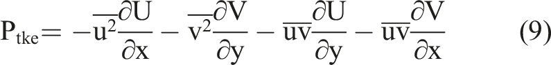
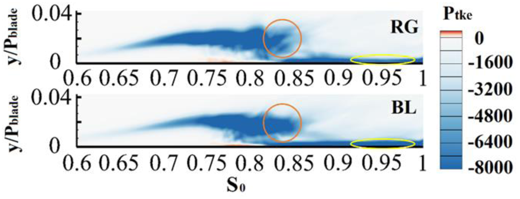
Comparison of ${\mathrm{P}}_{\text{tke}}$ .

As shown in the orange circle, the dark block extends to approximately 0.85S₀ under the BL case, while it is at approximately 0.82S₀ under the RG case. This may correspond to the effective impact of the KS on the K-H structure under the RG case in Figure 9. Moreover, as shown in the yellow circle, within the range of 0.9–1.0S₀, the height of the high ${\mathrm{P}}_{\text{tke}}$ region under the RG case is lower than that under the BL case, which also corresponds to the K-H structure. W1 remains undisrupted until arriving at the trailing edge under the BL case, as shown in Figure 9. ${\mathrm{P}}_{\text{tke}}$ provides good evidence for the foregoing analysis.

Summary

In this paper, the inflow condition of the lowest profile loss of a Pak-B profile is explored, and the traversal method is compared with an RBF-GA machine learning method. It is found that, under the same workload consumption, the effect of the RBF-GA method (RG) is better than that of the traversal method (BL). The RBF-GA method can be used for fine matching of high-lift low-pressure turbine design conditions.

The lowest profile loss found by the RG method is 0.214 lower than ${\mathrm{Y}}_{\mathrm{p}}^{*}$ of the BL method, resulting in a lower FSTI and lower Fr of the RG method. According to transient flow field analysis, the smaller blade profile loss in the RG case is due to the smaller wake angle of the RG case, which stimulates WCAKS closer to the leading edge of the blade. A strong WCAKS impact disrupts the K-H vortex induced by the WC in front of the trailing edge. Although WCAKS are generated under the BL case, WCAKS are generated in the middle on the blade surface, and there is not enough movement distance to strengthen them before interacting with the K-H structure. Therefore, a wake-induced transition of the boundary layer occurs later, resulting in a higher profile loss. At other times during the wake passage period, the momentum thicknesses at the trailing edge of the two cases are similar. The subtle difference in boundary layer flow results in a lower profile loss. Better inflow conditions can be explored by the machine learning method.