BiGlobal stability analysis of the wake behind an isolated roughness element in hypersonic flow

Abstract

Numerical results are presented for the stability analysis of the wake induced by a cuboidal roughness element mounted on a flat plate inside a Mach 6 freestream. Linear BiGlobal stability calculations are carried out for a single frequency on a spanwise plane located behind the roughness, using base flows obtained from laminar Navier–Stokes simulations. The results show that the Mack mode is the most unstable perturbation growing in the boundary layer, followed by varicose and sinuous deformations of the low-velocity streak that characterizes the wake flow structure. The shock wave induced at the leading edge of the flat plate is found to have a significant stabilizing effect on the flow field. The use of a higher wall temperature stabilizes the Mack mode but increases the growth rate of the varicose perturbation.

Introduction

Boundary layer transition is a critical factor in the design of high-speed vehicles. Turbulent boundary layers are characterized not only by increased skin friction, and hence drag, but also by large heat transfer rates that lead to challenging aerothermodynamic loads. The local turbulent heat flux in the surface of a conventional reentry body can be an order of magnitude larger than in the laminar regime. ¹ Although hypersonic boundary layer transition has been an active research topic for decades, the physical mechanisms involved in the process are not well understood yet. As a consequence, the existing transition prediction tools for practical hypersonic applications still rely mainly on empirical correlations. This fact has important implications in the design process, involving large safety factors that lead to oversizing of the thermal protection systems, with the consequent reduction of the payload capacity. In order to improve the transition prediction capabilities for the design of future high-speed applications, new methodologies involving a higher degree of flow physics for each particular case should be developed. According to Reshotko, ² the use of experimental-based correlations should be replaced by methods based on stability theory and transient growth considerations. Nowadays, global linear stability theory has become a viable tool for relatively simple geometries from the computational point of view, which is able to provide accurate results in the first stages of the transition process. ³

The presence of three-dimensional isolated roughness elements on the surface of a body—such as those encountered during an atmospheric entry due to factors like damaged heat shield tiles, gap fillers, or remains of contaminants—are known to have an important impact in the transition process. The perturbations generated by these elements can accelerate the growth of incoming disturbances and introduce additional instability mechanisms in the flow field, eventually leading to a premature occurrence of transition. For instance, global infrared observations of in-flight roughness-induced transition were performed during the last reentry of the Space Shuttle Endeavour by Horvath et al. ⁴ The results showed that boundary layer transition over the windward surface of the Orbiter started to take place in an asymmetric manner after the nose region. After data analysis, it was concluded that transition was most likely caused by some form of isolated roughness near the nose landing gear door.

Even if a physics-based prediction of roughness-induced transition is not available nowadays, recent experimental and numerical investigations^5–8 have considerably increased our knowledge. The flow structure in the wake behind discrete roughness elements is mainly characterized by strong counter-rotating vortices that persist a long distance downstream in the transitional wake. These vortices lift-up low-momentum fluid from the body surface and give rise to low-velocity streaks that are surrounded by regions of high wall-normal and spanwise shear. Given the strong inhomogeneity of the flow field in the wall-normal (y) and spanwise (z) directions, classical linear stability theory (LST) is no longer a valid technique for this problem. In order to obtain meaningful results, the amplitude functions considered in the stability analysis must be dependent on both y and z coordinates, with no restrictions on their shape. This approach, in which the perturbations are inhomogeneous in two spatial directions but homogeneous in the third one and in time, is hereby referred to as BiGlobal stability theory, as introduced by Theofilis. ⁹ A significant amount of high-speed roughness-induced transition investigations by means of global instability theory have been carried out in the recent years, both for supersonic and hypersonic flows and mostly for elements mounted on top of a flat plate. Groskopf et al. ⁵ performed temporal BiGlobal analyses of the stability of the wake behind isolated 3D cuboidal roughness elements in a Mach 4.8 boundary layer, and compared the results against direct numerical simulations (DNS), reporting a very good agreement of the disturbance amplitude shapes. Similar analyses were developed by De Tullio et al. ⁷ at Mach 2.5 and by Paredes ¹⁰ and De Tullio and Sandham^8,11 at Mach 6 for the same configuration, in both cases comparing DNS results against spatial BiGlobal and PSE-3D stability theories. For the two studied cases, the two-dimensional eigenfunctions obtained from the BiGlobal stability computations and the growth rates extracted from the PSE-3D simulations were both found to be in close agreement with the DNS data. On the experimental side, Kegerise et al. ⁶ carried out measurements of the disturbance amplitudes behind a diamond element in a flat plate at Mach 3.5, and compared them against the spatial distribution obtained by the BiGlobal stability analyses of Choudhari et al.^12,13 with satisfactory results, thus reinforcing the validity of the theory for the cases considered. In all the investigations performed, the dominant wake instability modes were found to be varicose (even) and sinuous (odd) deformations of the low-velocity streak that characterizes the wake flow structure. Moving to a more practical configuration, Theiss and Hein ¹⁴ performed BiGlobal computations on the wake behind different roughness elements located on the heat shield of a reentry capsule in a Mach 5.9 freestream. For all their cases considered, the varicose wake modes were the most amplified in terms of maximum N-factors, with the cylindrical roughness element being the most effective shape. Similar findings were also reported by Theiss et al. ¹⁵ on an extended study including PSE-3D calculations on the same configuration.

In the present study we analyze, by means of BiGlobal stability theory, the instability of the wake induced by a sharp-edged cuboidal roughness element mounted on top of a flat plate in hypersonic flow. The freestream values considered are the high-Reynolds number run conditions of the von Karman Institute (VKI) H3 tunnel. ¹⁶ The effect of the flat plate leading edge on the instability characteristics of the flow is investigated by means of three different base flows, respectively corresponding to an infinite flat plate with no leading edge, a finite flat plate with a sharp leading edge and a third one with a circular (blunt) leading edge. Furthermore, the influence of wall temperature on the stability is also examined through two different wall temperature boundary conditions, namely, an isothermal wall at ambient temperature and an adiabatic wall.

Governing equations

The governing equations considered in this study are the Navier–Stokes equations for a Newtonian fluid. They constitute a system of nonlinear partial differential equations that expresses the fundamental laws of conservation of mass, momentum and energy of a fluid. Denoting the primitive variables of the fluid as density ρ, pressure p, temperature T, and velocity components u _i (i = 1, 2, 3), the system can be written in conservation form and in a Cartesian reference frame as

$$\frac{\partial \rho }{\partial t}+\frac{\partial (\rho u_i)}{\partial x_i}=0$$

(1)

$$\frac{\partial (\rho u_i)}{\partial t}+\frac{\partial (\rho u_i{u}_j)}{\partial x_j}+\frac{\partial p}{\partial x_i}-\frac{\partial {\tau }_{\mathit{ij}}}{\partial x_j}=0$$

(2)

$$\frac{\partial (\rho E)}{\partial t}+\frac{\partial (\rho E{u}_i+p{u}_i)}{\partial x_i}+\frac{\partial q_i}{\partial x_i}-\frac{\partial (u_i{\tau }_{\mathit{ij}})}{\partial x_j}=0$$

(3)

where t is the time coordinate, x _i is the ith spatial coordinate and $E=e+u_i{u}_i/2$ , with e being the specific internal energy of the fluid. The viscous stress tensor τ _ij is defined as

$${\tau }_{\mathit{ij}}=\mu (\frac{\partial u_i}{\partial x_j}+\frac{\partial u_j}{\partial x_i}-\frac{2}{3}\frac{\partial u_k}{\partial x_k}{\delta }_{\mathit{ij}})$$

(4)

where μ is the dynamic viscosity of the fluid and δ _ij is the Kronecker delta. The conductive heat flux vector q _i is modeled using Fourier's law of heat conduction, given by

$$q_i=-k\frac{\partial T}{\partial x_i}$$

(5)

with k denoting the thermal conductivity of the fluid. Under the assumption of a calorically perfect gas, the system is closed through the perfect gas equation of state together with two additional thermodynamic relationships, respectively expressed as

$$p=\rho \mathit{RT},e=c_{v}T\text{\hspace{1em}and\hspace{1em}}{c}_v=\frac{R}{\gamma -1}$$

(6)

where R is the specific gas constant, c _v is the specific heat at constant volume, and γ is the ratio of specific heats. Here, air is considered with the values $\gamma =1.4$ and R = 287.18 J/(kg·K). Sutherland's law is used to account for the variation of the dynamic viscosity with temperature, such that

$$\mu ={\mu }_{\mathit{ref}}(\frac{T}{T_{\mathit{ref}}}{)}^{3/2}\frac{T_{\mathit{ref}}+S}{T+S}$$

(7)

with S = 110.4 K and the reference values ${\mu }_{\mathit{ref}}=1.716\times {10}^{-5}$ kg/(m·s) and T _ref  = 273.15 K. Furthermore, the Prandtl number is assumed constant with a value of Pr = 0.72, so that the corresponding thermal conductivity is calculated as $k=\mu c_p/\mathit{Pr}$ , where c _p denotes the specific heat at constant pressure. The similarity parameters that define the problem are γ and the freestream Reynolds, Mach, and Prandtl numbers, respectively denoted by $R{e}_{\infty },M_{\infty }$ , and $P{r}_{\infty }$ .

Formulation of the linear stability problem

Following classical linear stability theory, the primitive flow variables $\mathbf{q}=[u,v,w,T,p]T$ are split into a steady reference state $\overline{\mathbf{q}}$ , also known as base flow, and a small unsteady perturbation field $\stackrel{\sim }{\mathbf{q}}$

$$\mathbf{q}=\overline{\mathbf{q}}+\epsilon \stackrel{\sim }{\mathbf{q}}$$

(8)

with $\epsilon <<1$ . The base flow is assumed to be locally parallel in the streamwise (x) direction, so that $\overline{\mathbf{q}}=\overline{\mathbf{q}}(y,z)$ at a given x coordinate. As stated before, due to the high shear that characterizes the wake base flow in the wall-normal and spanwise directions, the amplitude of the perturbations is considered to be a function of both y and z. The ansatz of the modal perturbations for this case can be written as

$$\stackrel{\sim }{\mathbf{q}}(x,y,z,t)=\hat{\mathbf{q}}(y,z)\text{exp}[i(\alpha x-\omega t)]+c.c.$$

(9)

where $\hat{\mathbf{q}}$ is a vector containing the two-dimensional amplitude functions, α is the wavenumber along the streamwise direction, ω is the angular frequency and $c.c.$ denotes the complex conjugate.

In this work, the spatial approach is considered. In such a framework, ω is real and represents the angular frequency of the perturbations. On the contrary, α is complex, with the real part ${\alpha }_r=F\{\alpha \}$ being the streamwise wavenumber of $\stackrel{\sim }{\mathbf{q}}$ and the imaginary part ${\alpha }_i=F\{\alpha \}$ its spatial growth rate. With this definition, a positive value of α _i means a spatial decay of the amplitude function whereas ${\alpha }_i<0$ implies spatial growth.

The governing equations of the linear stability problem are obtained by substituting the ansatz in equation (9) into the Navier–Stokes system (equations (1) to (3)), then subtracting the base flow components and finally neglecting the nonlinear terms, which are of order $\mathcal{O}({\epsilon }^2)$ . In the end, the resulting linear system of partial differential equations can be written in the following compact form

$$\mathbf{A}\hat{\mathbf{q}}=\alpha \mathbf{B}\hat{\mathbf{q}}+{\alpha }^2\mathbf{C}\hat{\mathbf{q}}$$

(10)

where A, B, and C are complex and nonsymmetric differential matrix operators. After discretization of equation (10), an algebraic generalized eigenvalue problem (GEVP) is obtained, which is nonlinear in the eigenvalue α. The problem is linearized by means of the companion matrix method, ¹⁷ defining the following auxiliary vector: ${\hat{\mathbf{q}}}^{+}=[\hat{u},\hat{v},\hat{w},\hat{T},\hat{p},\alpha \hat{u},\alpha \hat{v},\alpha \hat{w},\alpha \hat{T}]T$ , so that the two-dimensional GEVP becomes

$${\mathcal{A}}^{+}{\hat{\mathbf{q}}}^{+}=\alpha {\mathcal{B}}^{+}{\hat{\mathbf{q}}}^{+}$$

(11)

with

$${\mathcal{A}}^{+}=[\begin{array}{cc}\mathcal{A}& \hfill -{\mathcal{B}}_{\hat{u}:\hat{T}}\hfill \\ 0& \hfill \mathbf{I}\hfill \end{array}]\text{\hspace{1em}and\hspace{1em}}{\mathcal{B}}^{+}=[\begin{array}{cc}{\mathcal{B}}_{\hat{p}}& \hfill {\mathcal{C}}_{\hat{u}:\hat{T}}\hfill \\ \mathbf{I}& \hfill 0\hfill \end{array}]$$

(12)

in which $\mathcal{A}$ denotes the discrete matrix operator associated to matrix A. ${\mathcal{B}}_{\hat{u}:\hat{T}}$ and ${\mathcal{C}}_{\hat{u}:\hat{T}}$ are nonsquare matrices that contain the columns from the respective discrete operators $\mathcal{B}$ and $\mathcal{C}$ , which correspond to the variables $\hat{u},\hat{v},\hat{w}$ , and $\hat{T}$ . Similarly, ${\mathcal{B}}_{\hat{p}}$ is a square matrix that contains only the columns from $\mathcal{B}$ that correspond to the variable $\hat{p}$ and I is the identity matrix. It is important to note that this procedure significantly increases the size of the system to be solved (from 5 to 9 variables).

Numerical methodology

Calculation of the laminar base flow

The geometrical configuration analyzed here consists of a sharp-edged cuboidal roughness element mounted on top of a flat plate. The freestream values considered correspond to the high-Reynolds test conditions of the VKI H3 hypersonic wind tunnel, ¹⁶ which are summarized in Table 1. Because of the low freestream temperature (total temperature $T_0=500$ K) no high-enthalpy effects are expected in the flow, so the assumption of a calorically perfect gas is justified. Depending on the case, the flat plate wall is either considered to be isothermal, with a wall temperature of T _w  = 300 K, or adiabatic. The first option is a reasonable approximation of the situation encountered in the wind tunnel, characterized by short operating times, whereas the second one is more representative of flight conditions. The numerical solution of the base flow is fully laminar, and is carried out using the computational fluid dynamics package CFD++® ¹⁸ on a block-structured grid consisting of hexahedral cells, respectively obtained with OpenFOAM's blockMesh ¹⁹ utility. The spatial discretization is based on a second-order upwind finite volume scheme, featuring a limited total variation diminishing (TVD) flux interpolation to minimize numerical oscillations in the vicinity of discontinuities. Regarding time integration, an implicit (backward Euler) scheme with multigrid acceleration is employed.

Table 1.

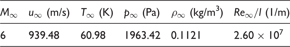
Summary of the freestream conditions used in the computations.

$M_{\infty }$	$u_{\infty }$ (m/s)	$T_{\infty }$ (K)	$p_{\infty }$ (Pa)	${\rho }_{\infty }$ (kg/m3)	$R{e}_{\infty }/l$ (1/m)
6	939.48	60.98	1963.42	0.1121	$2.60\times {10}^7$

A representation of the computational domain used to obtain the base flow is shown in Figure 1. As it can be observed, the domain is located below the shock wave induced at the flat plate leading edge, and can be considered to be a subset of a bigger domain, which includes the complete flat plate. This approach has already been used in similar analyses with successful results.^7,11,14 It helps to reduce the computational effort needed to obtain a converged base flow while adding flexibility to test different inflow conditions. Nevertheless, it requires the imposition of adequate inflow profiles at the inflow and top boundaries, which usually come from another numerical solution of the Navier–Stokes equations or from a self-similar boundary layer ²⁰ computation. The top boundary has a slope in order to avoid roughness-induced shock waves to impinge on it, at an angle given by the corresponding Mach wave for the freestream conditions: $\theta =\mathit{arcsin}(1/M_{\infty })\approx 9.{59}^{\circ }$ . Furthermore, due to the spanwise symmetry of the geometry under study, only half of the element is considered. The size and location of the roughness element are determined following the approach of De Tullio et al., ⁷ in which the roughness has a height (h) equal to the displacement thickness of the boundary layer ( ${\delta }^{*}$ ) at a location defined by the Reynolds number $R{e}_{{\delta }^{*}}=u_{\infty }{\delta }^{*}/{\nu }_{\infty }$ and the freestream conditions. The value for $R{e}_{{\delta }^{*}}$ employed here is the same as the one used in that study, namely $R{e}_{{\delta }^{*}}=8200$ , which, with the freestream parameters considered, gives a roughness height of $h={\delta }^{*}=0.32$ mm. The planform shape of the roughness element is a square with edge length $d=6h$ . The leading edge of the roughness is placed at a streamwise distance of 34h from the inlet of the computational domain, which is in turn located at a streamwise distance of 16h measured from the streamwise position where the displacement thickness of the self-similar boundary layer matches ${\delta }^{*}$ . Using a self-similar boundary layer profile based on the conditions given in Table 1 with an isothermal wall at T _w  = 300 K, the inlet of the domain is determined to be located at x _in  = 2.03 cm with respect to the flat plate leading edge. As for the size of the computational domain, the streamwise and spanwise lengths are respectively $L_x=150h$ and $L_z=20h$ , and the domain height at the location of the roughness leading edge is $L_y=10h$ .

Figure 1.

Schematic representation of the problem geometry and the computational domain used to calculate the base flow for the stability analysis (not to scale).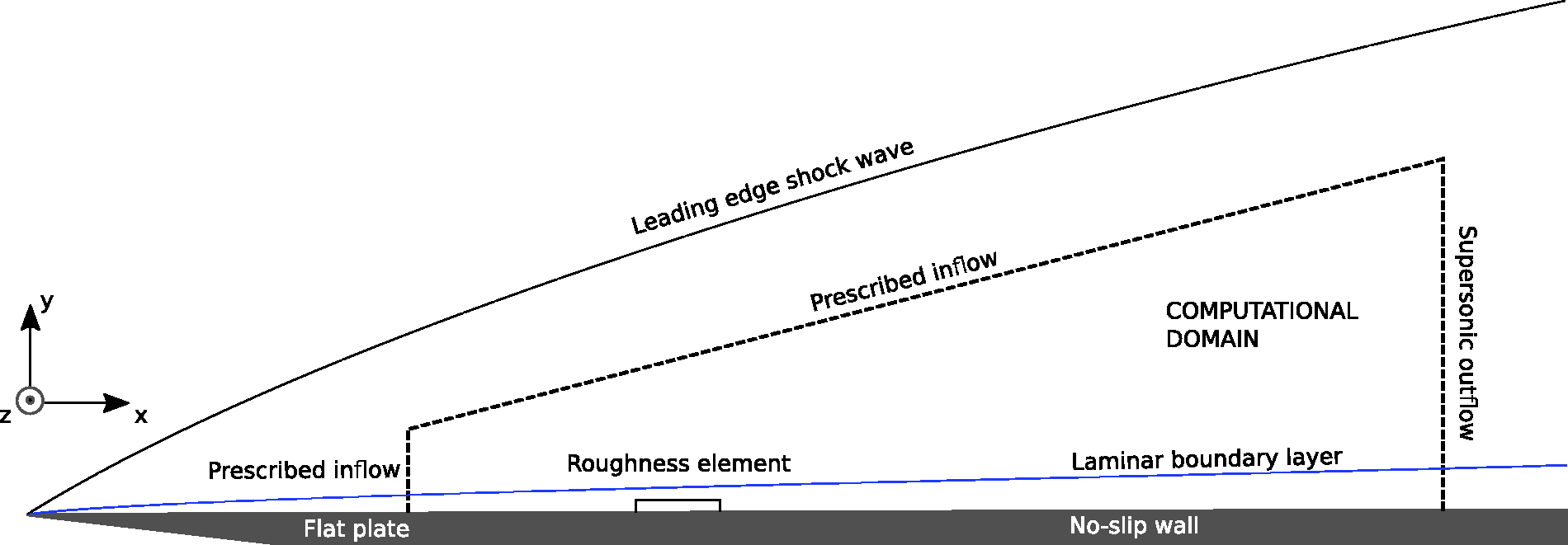

Regarding the boundary conditions, the primitive flow variables are prescribed at the inlet and the top boundaries of the domain with values that are either obtained from a converged numerical solution in a bigger domain without the roughness element or from a self-similar boundary layer computation. Note that when no roughness is present, the flow field is constant along the spanwise direction and the problem becomes two-dimensional, so that the values to prescribe can be computed through a 2D simulation. This is an additional advantage of using a subdomain with prescribed inflow data. At the center and side planes, symmetry conditions are specified, such that the actual problem would correspond to a spanwise array of discrete elements. At the wall, a no-slip condition is enforced. Finally, at the outlet boundary a supersonic outflow condition is specified, in which all the primitive flow variables are extrapolated from the interior of the domain. With respect to the initial conditions, the flow field is initialized with the freestream values and the system is integrated in time until a decrease of eight orders of magnitude in the averaged residual is achieved.

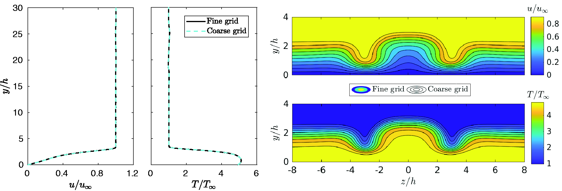
An overview of the numerical grid employed to calculate the base flow is represented in Figure 2, in the region surrounding the roughness element. In order to maintain a reasonable computational effort, the mesh is clustered towards the element in all directions. The cell spacing is uniform up to the roughness height in the wall-normal direction and up to the roughness width in the spanwise coordinate. From then on, a constant expansion ratio is applied until the domain boundary, always keeping a continuity in the cell sizes between the uniform and the expansion regions. In the streamwise direction, the grid is respectively clustered towards the leading and trailing edges of the roughness, also employing a constant expansion ratio. The ratios are uniquely defined by the number of cells desired on a given edge and the length of that edge. Under these considerations, the number of respective cells in the streamwise, wall-normal, and spanwise directions is 560, 340, and 240, resulting in a total count of about 43 million cells. In order to check the convergence of the base flow, an additional computation has been carried out on a finer mesh by increasing the number of points in the streamwise and wall-normal directions by 25%, reaching a total of 70 million cells. For a case prescribing the self-similar boundary layer solution at the inflow and top boundaries, Figure 3 shows a comparison of the boundary layer profiles at the roughness centerline and the streamwise velocity and temperature contours on a spanwise plane, all of them evaluated at the domain outlet for the two different meshes. It can be seen that both grids give the same base flow results, so the coarser mesh has been employed in all the computations reported in this work.

Figure 2.

Detail of the computational grid used to obtain the base flow in the region near the roughness element. Only every four grid points in the streamwise and spanwise directions and every six in the wall-normal direction are shown.

Figure 3.

Comparison of the base flow obtained with the designed grid and a finer grid with a 25% increase in the number of cells in the streamwise and wall-normal directions, for a case prescribing the self-similar boundary layer at the inlet and top boundaries. (Left) Boundary layer velocity and temperature profiles at the roughness centerline (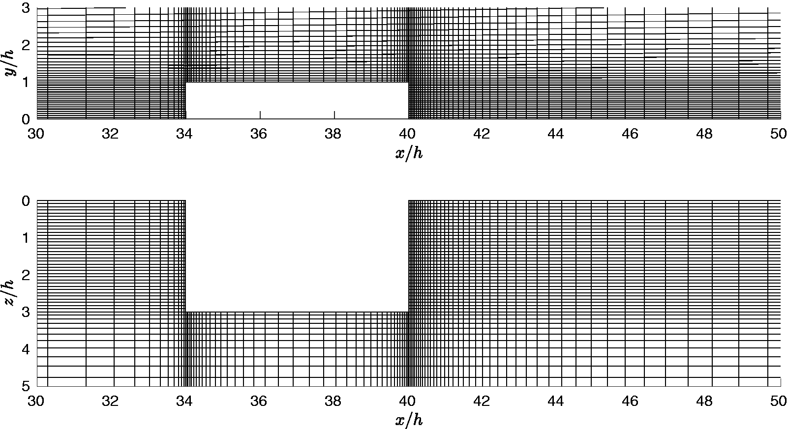 $z/h=0$ ) at the domain outlet ( $x/h=150$ ). (Right) Contours of streamwise velocity and temperature at the outlet spanwise plane.

Solution of the generalized eigenvalue problem

The numerical solution of the stability problem given by equation (10) is performed using VKI's Extensible Stability & Transition Analysis (VESTA) toolkit, originally developed by Pinna.^21,22 The particular structure of the matrices A, B, and C is automatically derived and implemented in MATLAB®²³ by means of a tool based on the Maxima ²⁴ computer algebra system. The 2D partial differential eigenvalue problem resulting from the BiGlobal approach is discretized by means of the Chebyshev collocation method. ²⁵ This technique is based on a Lagrange polynomial interpolation in a structured grid with a non-uniform point distribution given by the Chebyshev–Gauss–Lobatto collocation points, defined on a transformed domain with spanwise and wall-normal coordinates respectively denoted by ξ and η, with $\xi ,\eta \in [-1,1]$ . It has to be noted that the computational domain for the stability analysis of interest consists of a spanwise plane orthogonal to the flat plate wall, so the use of a rectangular grid is suitable for the solution. In the majority of practical problems, the transformed grid does not coincide with the physical domain under study, and therefore adequate geometrical mappings have to be considered. In the computations presented in this work, the mapping originally introduced by Malik ²⁶ is applied, which allows placing half of the grid points below a given location. For the wall-normal direction, the transformation is given by

$$y=\frac{y_i{y}_{\text{max}}(1+\eta )}{y_{\text{max}}-\eta (y_{\text{max}}-2y_i)}$$

(13)

where y _max is the coordinate at which the stability domain is truncated and y _i denotes the location where the number of discrete points is split into two halves. The same mapping is also applied along the spanwise coordinate. In this way, the grid used for solving the stability problem is clustered towards the boundary layer and the roughness centerline, which are the regions where the strongest base flow gradients are encountered. Even though equation (13) transforms the stability grid into the physical domain, the mapped grid defined by the Chebyshev–Gauss–Lobatto collocation points does not coincide with the mesh employed to obtain the base flow solution in this work. Therefore, before proceeding to build the eigenvalue problem, the base flow data is interpolated on the collocation grid by means of a cubic spline interpolation in each spatial direction.

Before solving the discrete GEVP, appropriate boundary conditions must be set for the perturbations. At the wall, the no-slip condition is enforced by setting the velocity perturbations to zero by means of a homogeneous Dirichlet condition. The same is also applied for the wall temperature disturbance, whereas the pressure fluctuation is determined by means of a compatibility condition satisfying the wall-normal momentum equation at $y/h=0$ . In the wall-normal far-field boundary, the perturbations are forced to decay by also imposing a Dirichlet boundary condition. Regarding the spanwise boundaries, the symmetry of the problem is again exploited in order to reduce the computational effort. In both the centerline and the spanwise far-field boundaries, symmetry or antisymmetry boundary conditions are specified. In the antisymmetric case, all the disturbances are set to zero except the spanwise velocity perturbation ( $\stackrel{\sim }{w}$ ), whose derivative normal to the boundary must be null. The latter is achieved through a homogeneous Neumann boundary condition. On the other hand, for the symmetric case the previous considerations are inverted, so that Neumann conditions are specified for $\stackrel{\sim }{u},\stackrel{\sim }{v},\stackrel{\sim }{T}$ , and $\stackrel{\sim }{p}$ , and Dirichlet for $\stackrel{\sim }{w}$ .

The classical algorithm for solving generalized eigenvalue problems is the QZ method, ²⁷ which is able to compute the complete eigenvalue spectrum. Nevertheless, its computational cost makes it feasible only for the solution of small problems. For the cases investigated in this work, the discrete matrices ${\mathcal{A}}^{+}$ and ${\mathcal{B}}^{+}$ reach a dimension of order $\mathcal{O}({10}^5)$ , and as a result other options have to be considered. For such large-scale problems, the most common alternative is the implicitly restarted Arnoldi method, ²⁸ which is an iterative method that only provides a given number of eigenvalues in the vicinity of a specific region. The solver built in VESTA toolkit makes use of the parallel implementation of the algorithm given by the PARPACK library, ²⁹ which is written in Fortran, and employs the message passing interface (MPI) standard. The Arnoldi iteration works optimally for extracting eigenvalues near the boundaries of the spectrum. However, in the majority of situations the interest is focused on interior values that are closer to the origin. In order to modify the search region, the so-called shift-invert transformation is applied, which transforms the problem into the following one

$$({\mathcal{A}}^{+}-\sigma {\mathcal{B}}^{+})-1{\mathcal{B}}^{+}{\hat{\mathbf{q}}}^{+}=\nu {\hat{\mathbf{q}}}^{+},\text{ with }\nu =\frac{1}{\alpha -\sigma }$$

(14)

where σ is the shift-invert parameter, around which the eigenvalues are sought. The large matrix inversion involved in the solution process is based on a LU decomposition that is also performed in parallel by means of the Scalable Linear Algebra PACKage (ScaLAPACK) library. ³⁰ The current solver has been previously tested against experimental data in the case of wake instabilities behind a micro-ramp mounted on top of a flat plate in incompressible regime by Groot et al., ³¹ delivering satisfactory results.

Results

A summary of the different cases investigated in this work is provided in Table 2. The parameter Re _h denotes the roughness Reynolds number, defined as $R{e}_h=u_{h}h/{\nu }_h$ , where u _h and ν _h are the streamwise velocity and the kinematic viscosity of the fluid evaluated at the streamwise location of the roughness leading edge and at a height of $y/h=1$ . Typical values reported in the literature above which transition starts to take place range around $R{e}_h\approx 300-500$ . ¹⁴ The value of $h/{\delta }_{99}$ describes the ratio between the roughness height (h) and the local boundary layer thickness at the streamwise position of the leading edge of the roughness element, denoted by δ₉₉. The value of δ₉₉ is determined by means of the total enthalpy criterion $h_0/h_{0,\infty }=0.995$ , ³² using the inflow data boundary layer profiles associated to each particular case. On the one hand, cases 1 to 3 are used to study the effect of the flat plate leading edge on the instability of the wake. The only difference between them is the inflow data that is prescribed at the inlet and the top boundaries of the domain, namely, the self-similar boundary layer profile, the solution from a 2D CFD simulation considering a flat plate with a sharp leading edge, and the flow resulting from another 2D computation assuming a flat plate with a circular leading edge of radius r = 0.5 mm. On the other hand, in case 4 the wall is assumed to be adiabatic while keeping the rest of the parameters identical to the first set-up. This last case is used to assess the influence of the wall temperature on the instability characteristics of the flow. The adiabatic wall temperature of the self-similar boundary layer can be estimated through the approximate relation ²⁰ $T_{\mathit{ad}}/T_{\infty }=1+P{r}^{1/2}[(\gamma -1)/2]M_{\infty }^2$ , which, with the parameters used in this work, gives a value of $T_{\mathit{ad}}\approx 434$ K. Therefore, the use of the ambient temperature (T _w  = 300 K) corresponds to a cold wall boundary condition.

Table 2.

Summary of the different cases analyzed.

Case	Wall temperature BC	Re h	$h/{\delta }_{99}$	Inflow data
1	Isothermal (T w  = 300 K)	324	0.54	Self-similar boundary layer
2	Isothermal (T w  = 300 K)	362	0.54	Smooth flat plate with sharp leading edge
3	Isothermal (T w  = 300 K)	297	0.47	Smooth flat plate with circular leading edge (r = 0.5 mm)
4	Adiabatic	138	0.44	Self-similar boundary layer

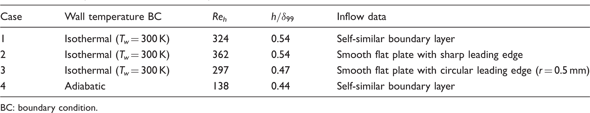
BC: boundary condition.

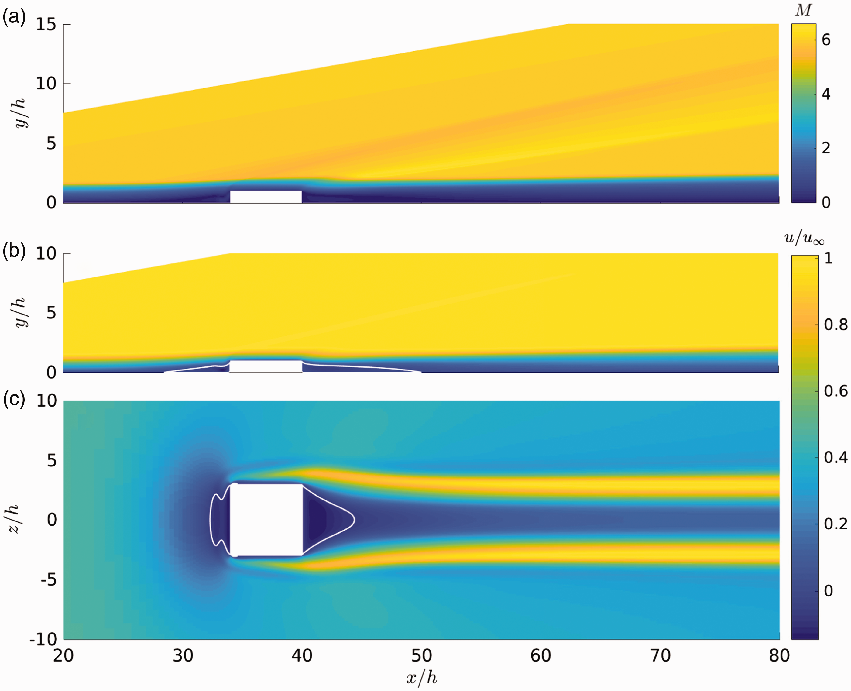
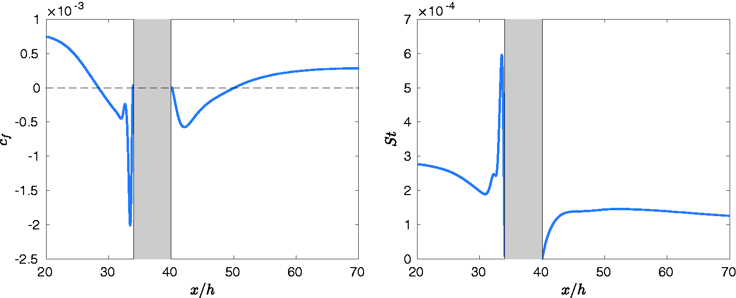
The main features of the base flow are depicted in Figure 4, which shows results for case 1. The roughness creates two regions of separated flow, located immediately upstream and downstream of it. As it can be observed, this low-velocity fluid causes a significant displacement of the boundary layer and induces a compression wave in the upstream region of the roughness leading edge, which eventually develops into an oblique shock further downstream. As the flow turns over the top of the roughness, an expansion wave is generated, immediately followed by a fan of compression waves that merges into an additional oblique shock as the flow reattaches downstream of the element. A more detailed representation of the separated flow regions can be obtained by looking at the skin friction coefficient and the Stanton number distributions along the flat plate wall. Here, the following definitions are employed

$$c_f=\frac{{\tau }_w}{\frac{1}{2}{\rho }_{\infty }{u}_{\infty }^2}$$

(15)

$$\mathit{St}=\frac{q_w}{u_{\infty }{\rho }_{\infty }{c}_p(T_w-T_{\infty })}$$

(16)

where τ _w and q _w are respectively the viscous shear stress and the magnitude of the heat flux at the flat plate wall. Figure 5 represents the skin friction coefficient and Stanton number distributions along the flat plate wall and at the roughness centerline for case 1. Negative values of the skin friction coefficient delimit the extent of the upstream and downstream detached flow regions. Both curves feature a strong peak in the upstream recirculation bubble generated in front of the roughness, which is a consequence of the significant blockage produced by the element and denotes a region of strong viscous dissipation. The downstream recirculation bubble, on the other hand, presents much lower values of skin friction as well as the lowest Stanton number.

Figure 4.

Base flow results for case 1. (a) Mach number contours on the streamwise (xy) plane at the roughness centerline ( $z/h=0$ ), showing the roughness-induced shock and expansion waves. (b) Streamwise velocity contours at the roughness center plane. (c) Streamwise velocity contours on a xz plane at $y/h=0.5$ . The white lines represent isolines of $u/u_{\infty }=0$ , delimiting regions of separated flow.

Figure 5.

Skin friction coefficient (left) and Stanton number (right) distributions along the flat plate wall at the roughness centerline ( $z/h=0$ ) for case 1. The shaded rectangular regions represent the location of the roughness element.

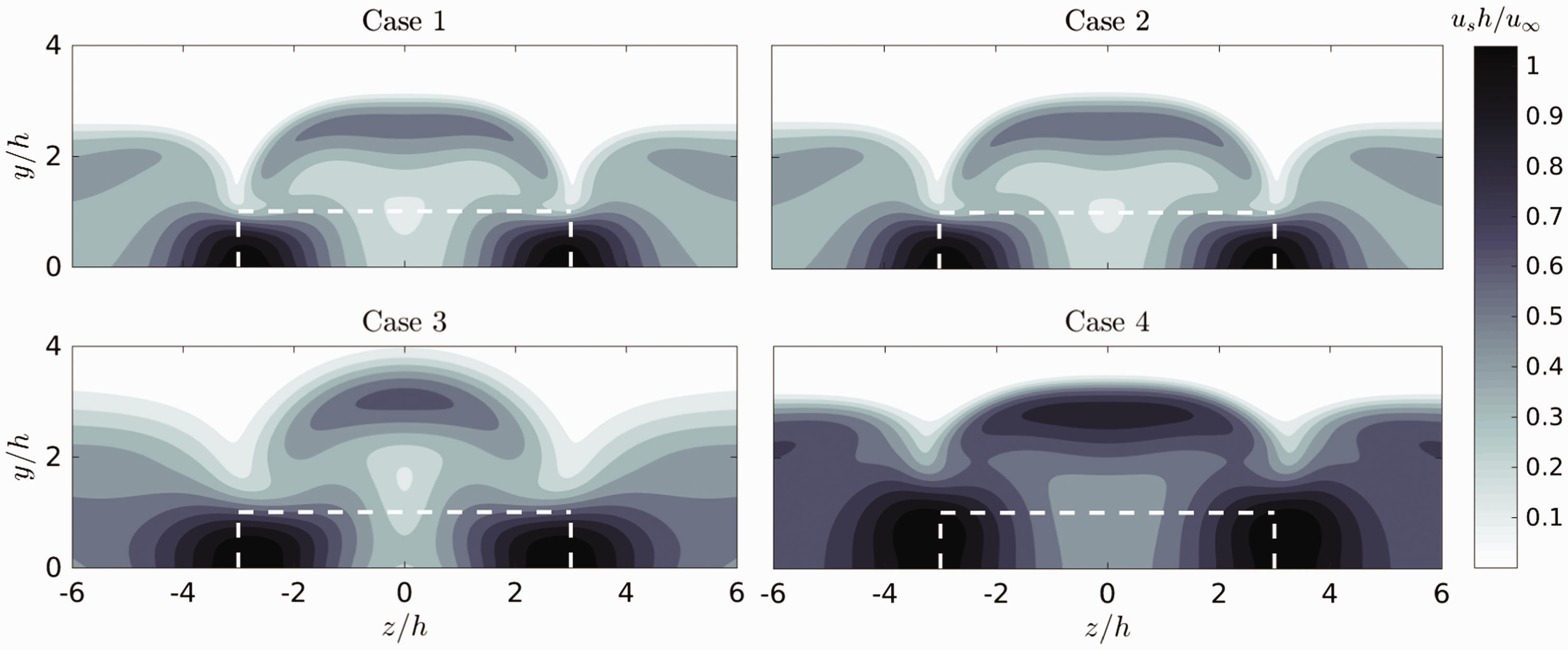
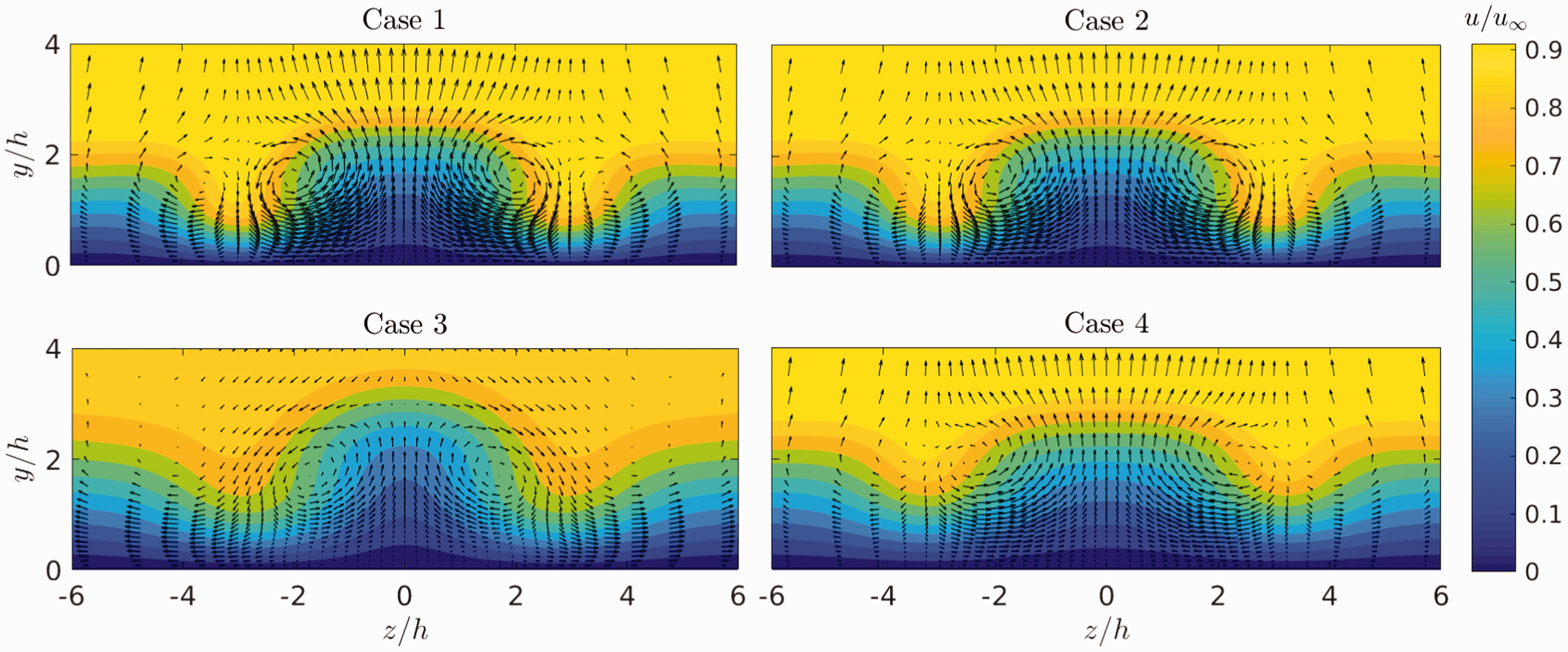
The spanwise structure of the flow field is presented in Figures 6 and 7. Figure 6 shows contour plots of the streamwise shear magnitude, defined as

$$u_s=\sqrt{(\frac{\partial u}{\partial y})2+(\frac{\partial u}{\partial z})2}$$

(17)

on a spanwise plane located at a distance of $\text{x}/\text{h}=140$ with respect to the inlet of the domain. Similarly, Figure 7 displays the corresponding two-dimensional velocity vectors (given by the v and w velocity components) on the same plane for each case, superimposed on contours of streamwise velocity. A pair of strong counter-rotating vortices can be identified, clearly visible in Figure 7 and also in the streamwise plane of Figure 4(c), which form at the edges of the roughness due to a pressure difference between the side and the top surfaces of the element. These streamwise structures lift-up low-momentum fluid from the surface of the flat plate and give rise to a mushroom-shaped low-velocity streak, ¹³ which is surrounded by regions of high-shear and large shear gradients in the wall-normal and spanwise directions, as displayed in the contour plots of Figure 6. It is also interesting to note in Figure 5 that due to this lift-up effect along the wake centerline, the skin friction coefficient and Stanton number asymptotic values in the far wake region are lower than far upstream of the roughness element (domain inlet).

Figure 6.

Contours of streamwise shear magnitude in a spanwise plane located at $x/h=140$ . The white dashed lines represent a projection of the roughness element.

Figure 7.

Two-dimensional velocity vectors superimposed on contours of streamwise velocity in a spanwise plane located at $x/h=140$ .

Regarding the spatial stability analysis, all the calculations are performed at a nondimensional frequency of F = 0.14, expressed as $F=\mathit{fh}/u_{\infty }$ , where f is the dimensional frequency, and at $x/h=140$ . The corresponding dimensionless angular frequency has a value of $\omega =2\pi F=0.88$ . These values have been chosen following the DNS results of De Tullio and Sandham ⁸ on a similar problem, where this frequency is the one with the highest disturbance growth rate and the plane is located at a streamwise distance where a significant linear development of the dominant instability modes has been attained. The mapping parameters considered for all the cases are as follows: $y_{\text{max}}/h=16,z_{\text{max}}/h=10,y_i/h=2.5$ and $z_i/h=2$ . All the spectra shown in this work contain the results of two different eigenvalue problems for each case, namely, the eigenvalues obtained with symmetry boundary conditions at the spanwise boundaries and the eigenvalues obtained with the antisymmetric counterpart.

Effect of the flat plate leading edge

Results of the stability calculation for case 1 are presented in Figures 8, 9, and 10. Figure 8 shows the spatial BiGlobal spectrum and the two-dimensional streamwise velocity amplitude functions—also known as eigenfunctions—of the most unstable discrete modes obtained at the specified streamwise location and frequency. In this case, the number of eigenvalues requested to the Arnoldi algorithm was 200 for each spanwise boundary condition specification (symmetry/antisymmetry), with a shift of $\sigma =0.95$ . Different grids have been tested in order to check the convergence of the spectrum with respect to the number of grid points in both the spanwise (N _z ) and the wall-normal (N _y ) directions, providing at the same time a direct visualization of the location of continuous, discrete and spurious numerical modes. A discretized vertical continuous branch located at ${\alpha }_r=\omega$ can be observed, which according to Balakumar and Malik, ³³ is composed of modes that represent entropy and vorticity waves. Although not shown in the picture, two additional horizontal continuous branches located in the real axis respectively at the right and left of the vertical branch can also be found in the spectrum. These branches are associated to the supersonic nature of the flow, and in this case represent acoustic waves. It has been checked that such branches can actually be retrieved when changing the shift of the transformed GEVP and/or solving for a larger number of eigenvalues. Several spurious modes appear scattered along the imaginary axis at a nearly constant wavenumber of about ${\alpha }_r=0.91$ , which do not show any grid convergence. Their unphysical nature has been further confirmed by looking at the associated amplitude functions. The discrete, and physically interesting, eigenvalues are located at the right of the continuous branch, spanning different wavenumbers in the range approximately between ${\alpha }_r=0.92$ and ${\alpha }_r=1$ . These modes are completely converged with respect to N _z , while convergence is close with respect to N _y , specially for the unstable eigenvalues. In the remaining stability calculations performed in this study, a grid resolution of 100 × 110 is employed.

Figure 8.

Spatial BiGlobal spectrum and contours of the normalized magnitude of the streamwise velocity eigenfunctions, $\left|\hat{u}\right|/\text{max}(|\hat{u}|)$ , for case 1 (F = 0.14, $x/h=140$ ). The letters in parenthesis associate the location of a given mode in the spectrum with its amplitude function. The eigenfunctions represented correspond to the case with 100 × 110 grid points.

Figure 9.

Contours of the normalized streamwise velocity perturbation on streamwise (xy) and wall-normal (xz) planes for the instabilities associated to the Mack mode in case 1, labeled (a), (b), (e), and (f) in Figure 8, at t = 0 s. The xz plots correspond to $y/h=2.44$ .

Figure 10.

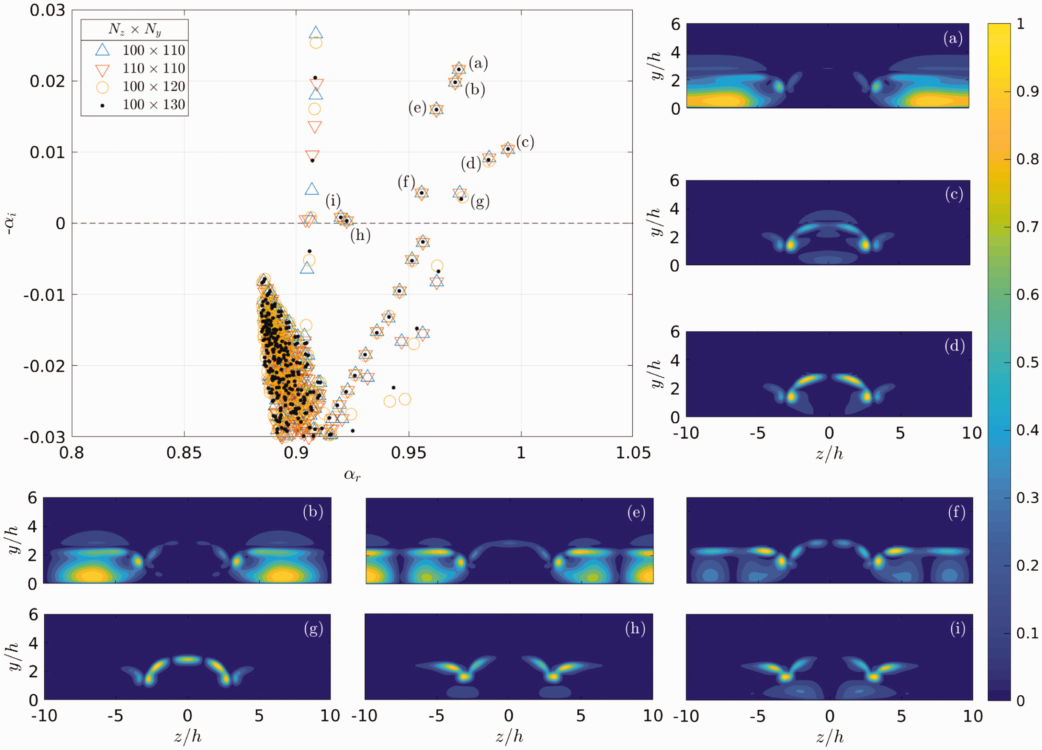
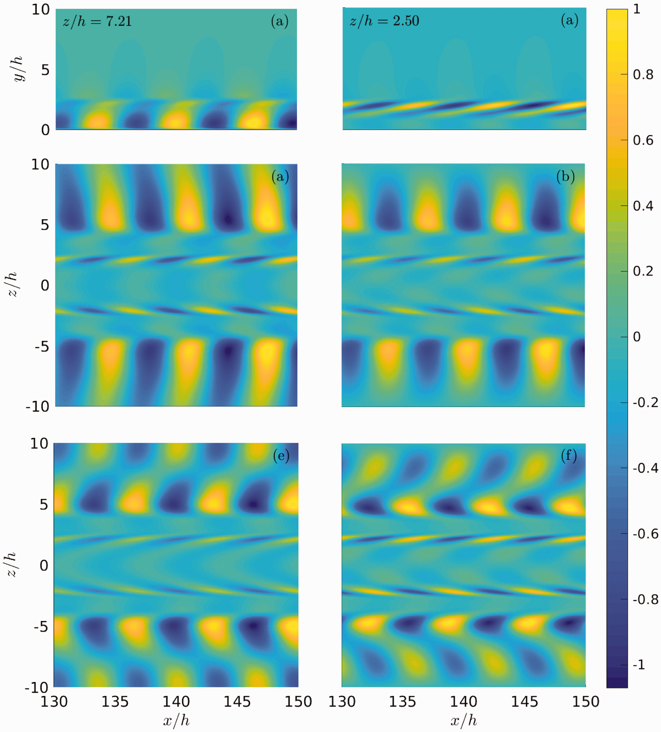
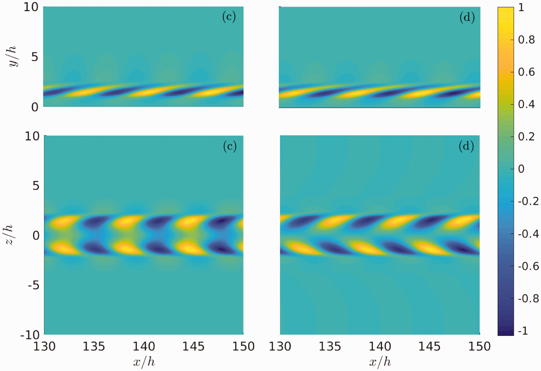
Contours of the normalized streamwise velocity perturbation on streamwise (xy) and wall-normal (xz) planes for the varicose and sinuous wake instabilities, labeled (c) and (d) in Figure 8, at t = 0 s. The xy plots correspond to $z/h=2.50$ and the xz plots to $y/h=2.69$ .

Nine unstable discrete modes are identified, labeled with letters from (a) to (i), respectively associated to the contour plots of the streamwise velocity amplitude functions. Figures 9 and 10 provide a more complete view of the three dimensional shape of the most relevant instabilities by displaying contour plots of the streamwise velocity perturbation ( $\stackrel{\sim }{u}$ ) on xy and xz planes along a streamwise region between $x/h=130$ and $x/h=150$ . The three-dimensional function $\stackrel{\sim }{u}=\stackrel{\sim }{u}(x,y,z,t)$ for each instability is obtained following the perturbation ansatz defined by equation (9), using the respective values of α and $\hat{u}$ computed by means of the BiGlobal solution at the selected location and frequency and at t = 0 s.

For the particular conditions considered, the leading instability mode (a) is the Mack mode, which mainly develops in the lateral boundary layer starting at the sides of the roughness element and spanning the complete computational domain in the spanwise direction. The nature of this mode is not associated to the presence of the roughness and therefore it can also be retrieved both with a BiGlobal analysis considering a clean flat plate or by means of classical linear stability theory. Nevertheless, in this case the wake induced by the element also contributes to the Mack mode perturbation, as can be observed in the xz plots and in the cut plane at $z/h=2.50$ in Figure 9, but with a lower amplitude. The second dominant instability mode (b) also peaks at the sides of the element, with an antisymmetric shape function showing a similar amplitude distribution to that of the Mack mode. The same is true for modes (e) and (f). It is argued that modes (b), (e), and (f) are oblique perturbations of the same family as the Mack mode, with an increasing spanwise wavenumber β ( ${\beta }_b<{\beta }_e<{\beta }_f$ ). Their diagonal-like distribution along the spectrum and the perturbation functions shown in Figure 9 support this argument. On the other side, modes (c) and (d) respectively correspond to the most unstable varicose and sinuous deformations of the low-velocity streak, whose amplitude functions are maximum in the high-shear layer surrounding the mushroom-shaped structure. These are the most unstable perturbations developing in the wake behind the roughness element, with the varicose mode showing a slightly higher growth rate in this case. Figure 10 shows the even and odd perturbation functions respectively associated with the varicose and sinuous instabilities as well as how their region of development is concentrated in the roughness wake and in the shear layer around the streak. The wake of the element also sustains the growth of two additional modes, denoted by (h) and (i), which have very small growth rates and their amplitude peaks are located at the interface between the streamwise vortices, the rising streak, and the lateral boundary layer. It is worth noting that, as could be expected, the regions where the amplitude functions of the wake modes are higher mainly correspond to the areas with larger shear magnitude gradients. Finally, mode (g) is associated to the leading wake fluctuations (c) and (d). Similarly to perturbations (b), (e), and (f) in the case of the Mack mode, this mode corresponds to an oblique ( $\beta >0$ ) instability of the same family as the varicose and sinuous modes, as can be observed by its wave-like amplitude function that surrounds the low-velocity streak. In fact, all the modes located in the diagonal line at the right of the vertical continuous branch are oblique variations of the varicose and sinuous deformations, with increasing β when moving towards lower growth rates. Mode (g) is the first oblique perturbation located in such diagonal branch.

The results obtained agree qualitatively well with the BiGlobal analysis of Paredes, ¹⁰ performed at the same frequency and streamwise position on a DNS base flow with the same roughness geometry and size but at different freestream conditions. In that study, the Mack mode is also the dominant instability mechanism, followed by the antisymmetric perturbation found in Figure 8(b) and the varicose mode, although no sinuous instability is reported. On the same problem, Van den Eynde and Sandham ³⁴ report that the varicose mode is linked to the development of the Mack mode and has a very similar nature, i.e. an acoustic mode that is trapped within the wake behind the roughness element and reflects back and forth between the wall and the sonic line of the low-velocity streak.

Focusing on the case with a sharp leading edge (case 2), it can be seen in Figure 6 that the base flow is very similar to that of case 1. Nevertheless, some small differences are noticeable, and the local thickness of the boundary layer is slightly higher than when the self-similar profile is considered. These discrepancies are more pronounced in the stability results, illustrated in the left plot of Figure 11, which shows a comparison of the spectrum obtained for cases 1 and 2. It can be seen that the shock induced at the flat plate leading edge is slightly stabilizing the boundary layer. Although the topology of the spectrum remains the same in both cases, all the discrete modes in case 2 have a lower growth rate than in case 1. Even if the leading edge shock is weak, it creates a small entropy gradient that produces a vorticity interaction of sufficient strength to modify the stability of the flow field. The stabilizing effect of the entropy layer is much stronger when a blunt leading edge is considered. The right plot in Figure 11 presents the resulting spectrum for the stability analysis of case 3. As it can be observed, no unstable modes have been retrieved for this case. It can be noticed in Figure 6 that the shear gradients that surround the low-velocity streak in case 3 are smaller than in the other configurations, already suggesting that the wake instability mechanisms might be considerably weaker. In order to confirm this result, on one side, a larger area of the BiGlobal spectrum has been scanned by performing BiGlobal stability computations with different shifts at a smaller resolution. On the other side, a LST analysis has been carried out at the lateral, low-disturbed boundary layer. None of the calculations have revealed unstable modes, so it is argued that the flow field is stable for this case at the particular frequency and streamwise position considered. The effect of the entropy layer on the linear stability of supersonic boundary layers over smooth blunt flat plates and cones was investigated by Balakumar. ³⁵ The reported findings show that the entropy layer that is formed in the bow shock induced by the blunt leading edge persists for a long distance downstream, leading to a strong stabilization of the boundary layer.

Figure 11.

(Left) Comparison of the spatial BiGlobal spectrum for cases 1 and 2. (Right) Spectrum for case 3. For clarity, spurious numerical modes are not shown.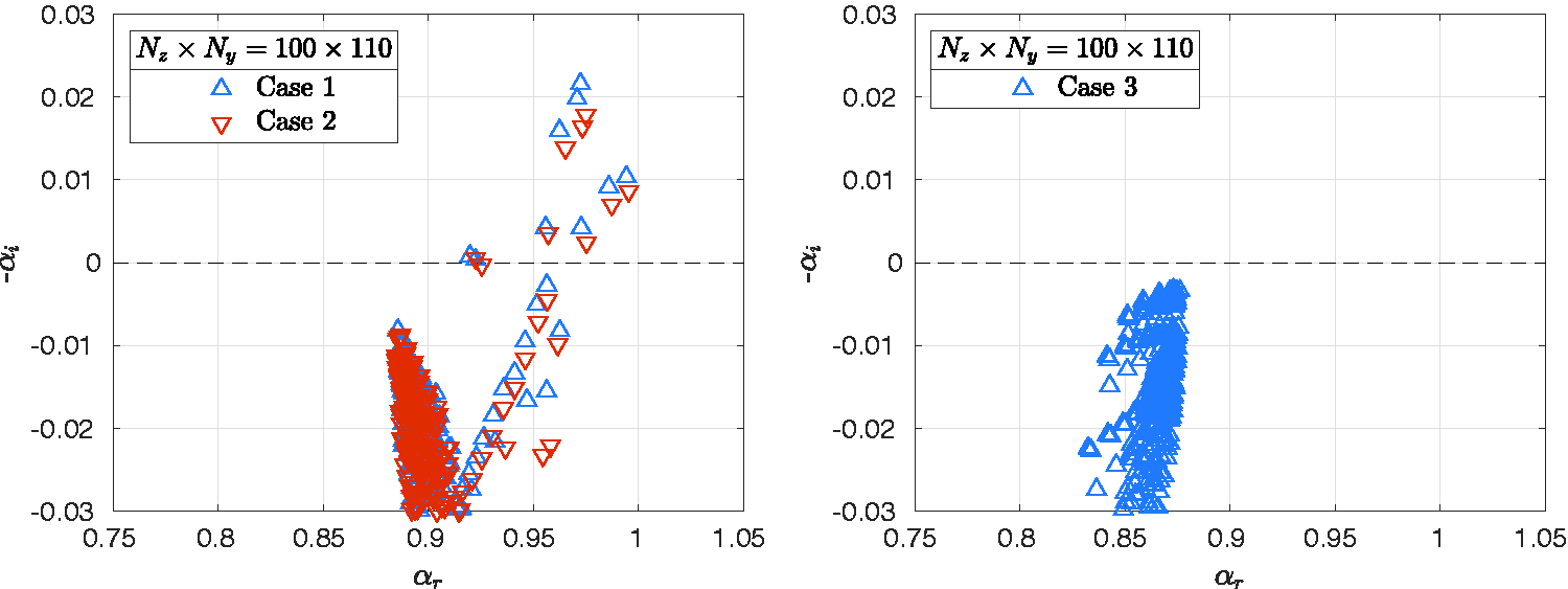

Effect of the wall temperature

The base flow obtained when considering an insulated flat plate (case 4) presents substantial differences with respect to the isothermal solution (case 1). As it can be seen in Figure 6, both the boundary layer and the roughness-induced vortices are considerably thicker when the wall is assumed to be adiabatic. This is expected owing to the higher wall temperature achieved in this case, since a larger volume of fluid is needed to accommodate the same mass flow due to the lower density. The shape of the streak is also modified, in this case having a region of increased streamwise shear in the upper part that is of similar magnitude as the shear produced by the counter-rotating vortices.

The results of the stability analysis performed to examine the effect of the wall temperature on the stability of the flow field are displayed in Figure 12. The eigenvalues obtained in case 1 are also shown in the spectrum to allow for a direct comparison. As before, the letters in parenthesis identify the unstable discrete modes. The topology of the spectrum and the eigenfunctions is very similar to the isothermal case, but the relative importance between the dominant instability modes presents some differences. In general terms, the boundary layer is more stable in this case. Focusing on the particular instability modes, the Mack mode (a) is once again the dominant perturbation, although with a lower growth rate than before. It is known from classical linear stability theory, see for instance Mack, ³⁶ that higher wall temperatures have a stabilizing effect on the Mack mode, thought to be due to the local decrease in the Mach number. The varicose (c) mode is, however, more unstable than in the previous case, and this time it has a very similar growth rate to the Mack mode, making it the second most unstable disturbance for this particular flow field. The amplitude function of the varicose mode presents a strong peak region in the upper part of the streak, associated to the increased shear appearing in the base flow in the same area. It is argued that this change in the low-velocity streak makes the wake more unstable, with the leading wake instability manifesting as a varicose deformation. On the contrary, the sinuous mode (d) is shifted down, becoming less unstable than when considering an isothermal wall. Modes (b), (e), and (f) once again correspond to oblique disturbances of increasing spanwise number that are associated with the Mack mode. The last mode (g) is of the same kind as modes (h) and (i) in case 1, namely, a disturbance peaking at the interface between the streak, the roughness-induced vortices and the lateral boundary layer.

Figure 12.

Spatial BiGlobal spectrum and contours of the normalized magnitude of the streamwise velocity eigenfunctions, 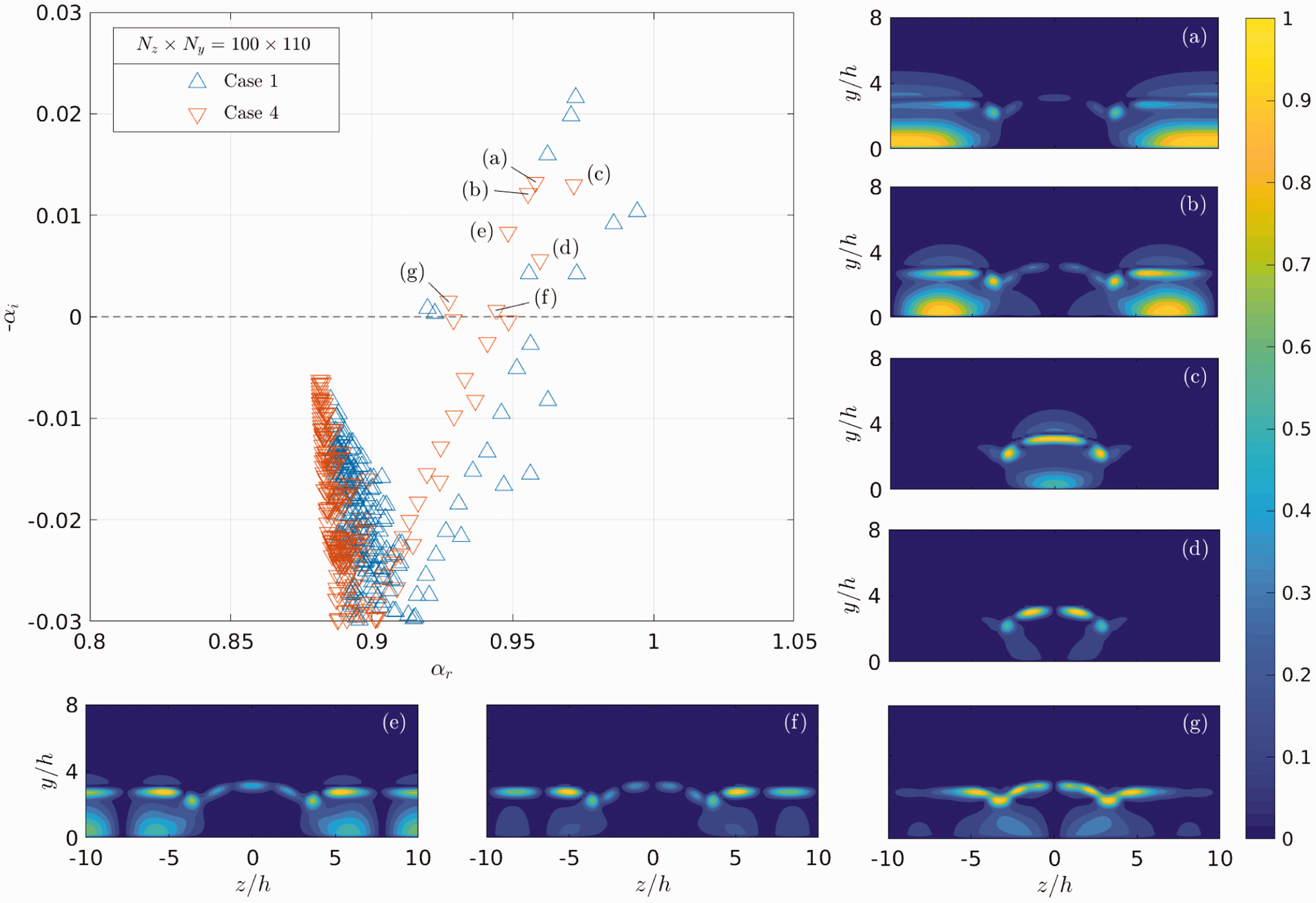$\left|\hat{u}\right|/\text{max}(|\hat{u}|)$ , for case 4 (F = 0.14, $x/h=140$ ). The letters in parenthesis associate the location of a given mode in the spectrum with its amplitude function. The resulting spectrum for case 1 is also displayed for comparison. For clarity, spurious numerical modes are not shown.

Conclusions

The instability of the wake behind a cuboidal roughness element mounted on a flat plate inside a Mach 6 freestream has been investigated using linear BiGlobal stability theory. The base flows employed have been obtained by means of perfect gas laminar Navier–Stokes simulations using a second-order accurate finite volume scheme. The roughness induces a strong counter-rotating vortex pair that gives rise to a mushroom shaped streak through the lift-up of low-velocity fluid from the flat plate surface. This structure is surrounded by regions of high shear stress and large shear gradients in the wall-normal and spanwise directions. The spatial growth rate and the two-dimensional amplitude functions of the instability mechanisms present in the flow have been computed at a particular nondimensional frequency of $\omega =0.88$ and at a streamwise position of $x/h=140$ from the domain inlet. At these conditions, the Mack mode is the most unstable perturbation growing in the boundary layer, followed by varicose and sinuous fluctuations that develop in the region surrounding the low-velocity streak that characterizes the wake. The amplitude functions of the wake instabilities are found to be maximum in the regions where the base flow has the strongest shear gradients. Different oblique instabilities associated to both the Mack and wake modes also present a significant growth, suggesting that they might as well play an important role in the transition process.

The effect of the flat plate leading edge on the stability characteristics of the flow field has been analyzed by considering sharp and blunt flat plates. The weak shock wave induced at the sharp leading edge turns out to have a noticeable stabilizing effect on the flow behind the element, attributed to the interaction between the entropy gradient generated by the small curvature of the shock and the boundary layer. The stabilization is much stronger when a blunt leading edge is assumed, up to the point that when a circular leading edge of radius r = 0.5 mm was used, the BiGlobal solution did not deliver any unstable discrete modes in the roughness-induced wake. The influence of the wall temperature has also been examined by comparing the stability results obtained with isothermal (T _w  = 300 K) and adiabatic ( $T_{\mathit{ad}}\approx 434$ K) wall boundary conditions. When the adiabatic wall is considered, the Mack mode is considerably stabilized, whereas the varicose perturbation becomes more unstable, approximately achieving the same growth rate as the Mack mode for the specific conditions under study.