Numerical investigation of aero-optical effects around the turret based on delayed detached eddy simulation and unsteady Reynolds averaged Navier-Stokes

Abstract

Delayed Detached Eddy Simulation (DDES) and Unsteady Reynolds Averaged Navier-Stokes (URANS), based on the two-equation Shear Stress Transport (SST) model, are implemented to investigate the flow features and the aero-optical distortions around the turret. The Mach number is Ma = 0.4 and the Reynolds number is Re = 1.43 × 10⁶. Instantaneous and time-averaged flow fields are presented to compare the ability of DDES and URANS in predicting the flow features. The instantaneous results show that DDES can resolve the abundant flow structures and more disordered density distributions than URANS. The time-averaged pressure coefficient and the density distribution of both methods are generally similar, but the time-averaged turbulent kinetic energy of URANS is far higher than that of DDES. The time-averaged pressure coefficient of DDES is closer to experimental data. In the windward view, typical surface flow features of DDES and URANS are similar. In the leeward view, there are remarkable differences of typical flow features between DDES and URANS. At the six angles of elevation, 60°, 76°, 90°, 103°, 120°, and 132°, the spatial-temporal wavefront distortions are calculated and discussed with the geometric ray-tracing method and the Zernike polynomial fitting, respectively. In spatial distribution, the wavefront distortions of DDES and URANS are slightly different from the experimental data. At the angles of 60°, 76°, 90°, and 103°, the tendencies of wavefront distortion of DDES at different tracing distances are the same with that of URANS, which is due to the same ability of two methods to resolve the density distributions in the attached flow region. However, the results of DDES agree well with the experimental results at the angles of 120° and 132°, which is bigger than the results of URANS. For temporal characteristics, the frequencies of wavefront distortions of DDES are obviously higher than that of URANS. The amplitudes of wavefront distortions by DDES are about 3 to 5 times higher than that by URANS. At the cases of two different FLHs at Ma = 0.4, the flow structures are totally similar, and the tendencies of wavefront distortion with θ are also similar. At the cases of three Mach number, the compression has a big influence on the wavefront distortion.

Introduction

Aero-optical effect is widely concerned with the adverse effects on laser beam transmission. When the laser beam passes through the inhomogeneous density field around the optical window, the offset, jittering, blurring, and energy attenuation of the laser beam could appear. ¹ When the laser beam passes through the fluctuant and inhomogeneous flow field, different parts of the laser beam propagate at different refractive index of the medium, causing the optical path difference (OPD). As shown in Figure 1, optical wavefront distortions are caused by two main aspects: one is the fluctuating turbulent flow near the optical window, and the other is the long-distance atmospheric propagation to the target.

Figure 1.

Schematics of laser beam passing through turbulence.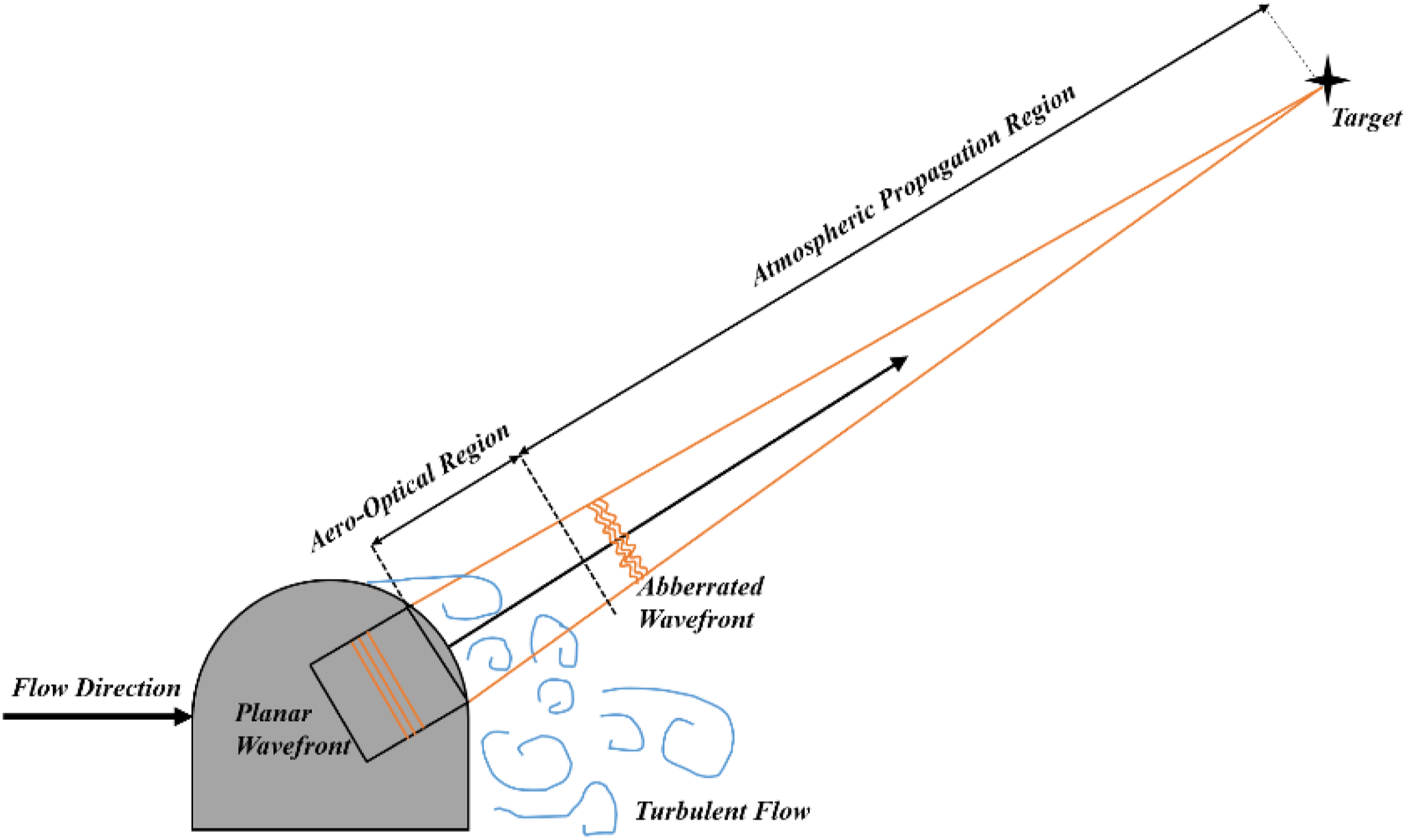

Due to the demand for laser weapon development, a mass of aero-optical experiments and numerical simulations were performed. So far, several typical flows, such as turbulent boundary layer,^2,3 free shear layer,^4,5 separated shear layer, and turbulent wake,^6,7 had been extensively studied. Many aero-optical systems had been designed. In particular, the hemisphere cylindrical turret attracted the most attention.^8,9,10 Many wind-tunnel tests and numerical simulations on the hemisphere cylindrical turrets had been conducted.

Gordeyev et al. ¹¹ experimentally investigated the aero-optical effect around a conformal-window turret and three sets of optical instruments were applied to measure the aberrations. The results showed that the use of the suite of sensors were able to distinguish between stationary disturbances and convective disturbances at the frequency of turret’s separated wake and the high frequencies associated with the structures in the separated shear layers, respectively. Cress et al. ¹² experimentally analyzed the aero-optical effects for back angles over flat windows on the three-dimensional hemispherical and two-dimensional cylindrical turrets. The results showed that the most aberrating aero-optical environments were caused by the separated flows. Lucca et al. ¹³ accomplished the local and global jitter measurements by two-dimensional wavefronts and accelerometer around the flat-window turret. The results showed that the aero-optical jitter was caused by the stationary and traveling aero-optical components. Detailed analysis of the global and the local jitter spectrum were also discussed. The comparison of pressure field over flat-window turret and conformal-window turret were discussed by Gordeyev et al. ¹⁴ Proper orthogonal decomposition (POD) was also used to extract dominant pressure modes. Several in-flight tests on the Airborne Aero-Optics Laboratory (AAOL) were conducted to obtain aero-optical data in the realistic flight with a three-dimensional hemisphere cylindrical turret.^15,16,17

Morgan and Visbal^18,19 used hybrid Reynolds Averaged Navier-Stokes (RANS)/implicit Large Eddy Simulation (ILES) and RANS simulations to resolve the flow over the three-dimensional turret. The hybrid RANS/ILES solution displayed complex flow phenomena in the wake of turret that RANS model is unable to resolve. The numerical results showed that it is the turbulent separation rather than the experimentally observed laminar separation that occurred from the top of the turret. However, the effects of hybrid method and RANS on the optical distortion were not discussed. Morgan et al. ²⁰ also accomplished resolving the flow around the turret by the high-order Navier-Stokes flow solver, and the results indicated that the flat window introduced moderate flow separation over most of the aperture. Jelic et al. ²¹ numerically simulated two typical turret geometries and the performance of the turrets for directed energy applications is inferred through the flow features, density and pressure fluctuations, and forces on the turrets. Mathew et al. ²² investigated the aero-optical effects over a hemisphere cylindrical turret by using large eddy simulation (LES). Comparisons were made between calculated aberration and previous experimental results, which showed reasonable agreement in trend and magnitude. Tang et al. ²³ and Malkus et al. ²⁴ investigated the flow around the turret using proper orthogonal decomposition (POD) and dynamic mode decomposition (DMD) and obtained the Strouhal number at different modes, but both articles did not study the fluctuation of aero-optical effects. Ren et al.^25,26 experimentally and numerically investigated the effects of an annular rough wall on the passive control of fluid and the aero-optics. The experimental results show that the steady wavefront distortions at the zenith with the rough wall at roughness k_s=1mm are 21%–50% smaller than those with smooth walls. However, the conclusions by Ren et al. are obtained from time-averaged wavefront distortion. General reviews of computational and experimental investigations can be found in the articles by Wang et al., ²⁷ Ding et al.,^28,29 and Jumper et al. ³⁰

Although many experimental and numerical investigations over the three-dimensional turrets have been accomplished, the investigations in this paper have some innovations. Most of articles pay attention to time-averaged wavefront distortion, but some temporal frequency characteristics are discussed in this article. Almost all articles investigated the spatial distribution of the aero-optical effects over the hemisphere cylindrical turret only at different angles, but this article study the change of aero-optical effects under different raytracing distances, which shows the change of wavefront distortion when the beam pass through the flow field. In addition, Zernike polynomial fitting is used to analyze the wavefront distortion. High-order components of wavefront distortion can be obtained by Zernike polynomial, so that we can compare the simulation results with the experimental results and ensure the accuracy of our simulation results. Surely, the comparation of URANS and DDES in calculating the aero-optical effects are valuable for engineering applications. Furthermore, the flow structures and aero-optical effects influenced by Mach number and first-layer height (FLH) are also briefly discussed.

Consequently, in this article, detailed analysis of the temporal frequency characteristics of the aero-optical effect is performed by Zernike polynomial fitting.^31,32 The spatial distribution characteristics of the aero-optical effect are also discussed at different ray-tracing distances. All of the flow field simulations are performed with the software ANSYS CFX, which is based on solving Navier-Stokes equations by the element-based finite volume method. In order to accurately predict the separated flow structures in the wake of the turret, the Delayed Detached Eddy Simulation (DDES) and the Unsteady Reynolds Averaged Navier-Stokes (URANS) method with the two-equation Shear Stress Transport (SST) turbulence model are implemented to resolve the flow around the turret. Compared with the wind-tunnel data obtained by Gordeyev et al., ¹¹ the detailed flow structures are also presented in this article.

Numerical methodologies

Numerical method

In the present study, both the URANS and DDES methods use the two-equation k-ω shear stress transport (SST) model as the turbulent model, which is developed by Menter. ³³ The model proposes a modification of the eddy viscosity to account for the transport of the turbulent shear stress. This model can not only provide a much more robust and accurate formula for the viscous sublayer, but also improve the calculation accuracy of boundary layers in adverse pressure gradients.

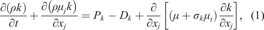
An improved version of DDES ³⁴ is applied in the present simulation. Since the DES method can be constructed through modification of the destruction term of the turbulent kinetic energy transport equation, ³⁵ the k-equation of DDES can be expressed as

$\frac{\partial \left(\rho k\right)}{\partial t}+\frac{\partial \left(\rho {\mu }_{j}k\right)}{\partial x_j}=P_k-D_k+\frac{\partial }{\partial x_j}\left[\left(\mu +{\sigma }_k{\mu }_t\right)\frac{\partial k}{\partial x_j}\right],$

(1)

where μ _t denotes the turbulent viscosity. The production term and the destruction term are given, respectively, by

$P_k={\tau }_{ij}\overline{S_{ij}},$

(2)

$D_k=\rho k^{3/2}/l_{DDES}.$

(3)

The hybrid length scale l _DDES can be expressed as

$l_{DDES}=\min \left(l_{RANS},\frac{l_{LES}}{1-F_{SST}}\right).$

(4)

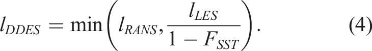
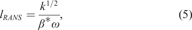
The hybrid length scale can switch between the turbulence length scale l _RANS and the filter length scale l _LES , which are expressed as

$l_{RANS}=\frac{k^{1/2}}{{\beta }^{*}\omega },$

(5)

$l_{LES}=C_{DES}{\mathrm{\Delta }}_{DDES},$

(6)

${\mathrm{\Delta }}_{DDES}=\max \left(\delta x,\delta y,\delta z\right),$

(7)

where ∆_DDES is related to the maximum local grid spacing as the filter width and β∗ denote a constant of the SST model developed by Wilcox. ³⁶ F _SST is a damping parameter of the SST model developed by Strelets. ³⁵ In the near-wall region with big adverse pressure gradients, F _SST is equal to one and forces the simulation to the RANS mode. Outside the boundary layer, F _SST turns to zero and switches the mode to the LES form. Notably, a special blending function proposed by Strelets ³⁵ allows the use of the High Resolution Scheme (HRS) in the RANS region and a second-order Central Difference Scheme (CDS) in unsteady and LES regions.

Simulation setup

The geometry implemented in this article was proposed as a benchmark test case for investigation of the laser beam weapon. The size of the turret geometry is obtained from Gordeyev’s test ¹¹ in the subsonic wind tunnel at the U.S. Air Force Academy (AFA). In this experiment, the aero-optical effects of the turret were measured from elevation angles θ between 60° and 132°. In the present work, the elevation angles of 60°, 76°, 90°, 103°, 120°, and 132°, are investigated.

The computational domain applied in this simulation takes the same form as the test section in the wind tunnel at AFA, depicted in Figure 2

Figure 2.

Schematics of the computational setup for the turret.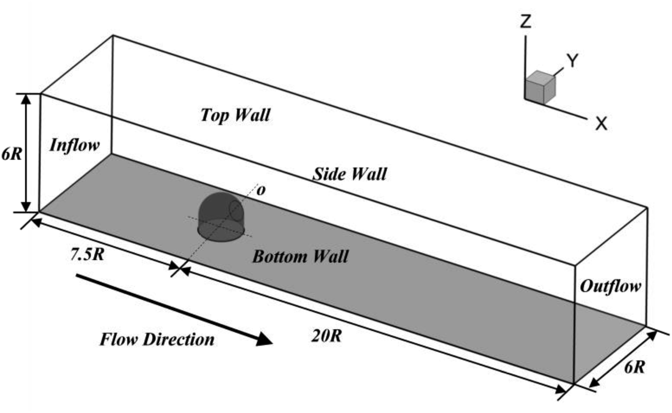

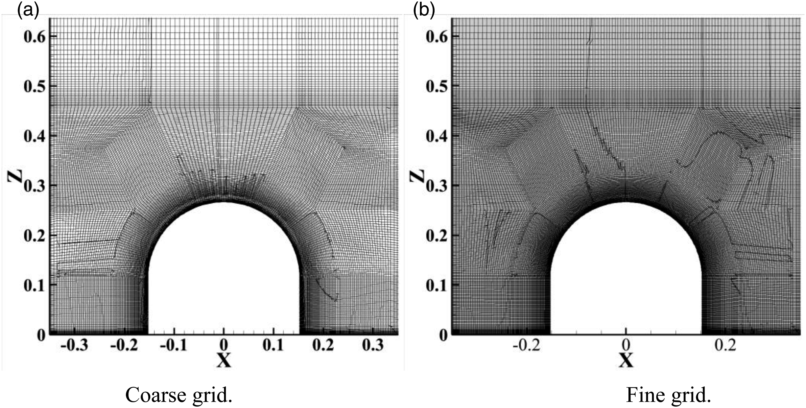
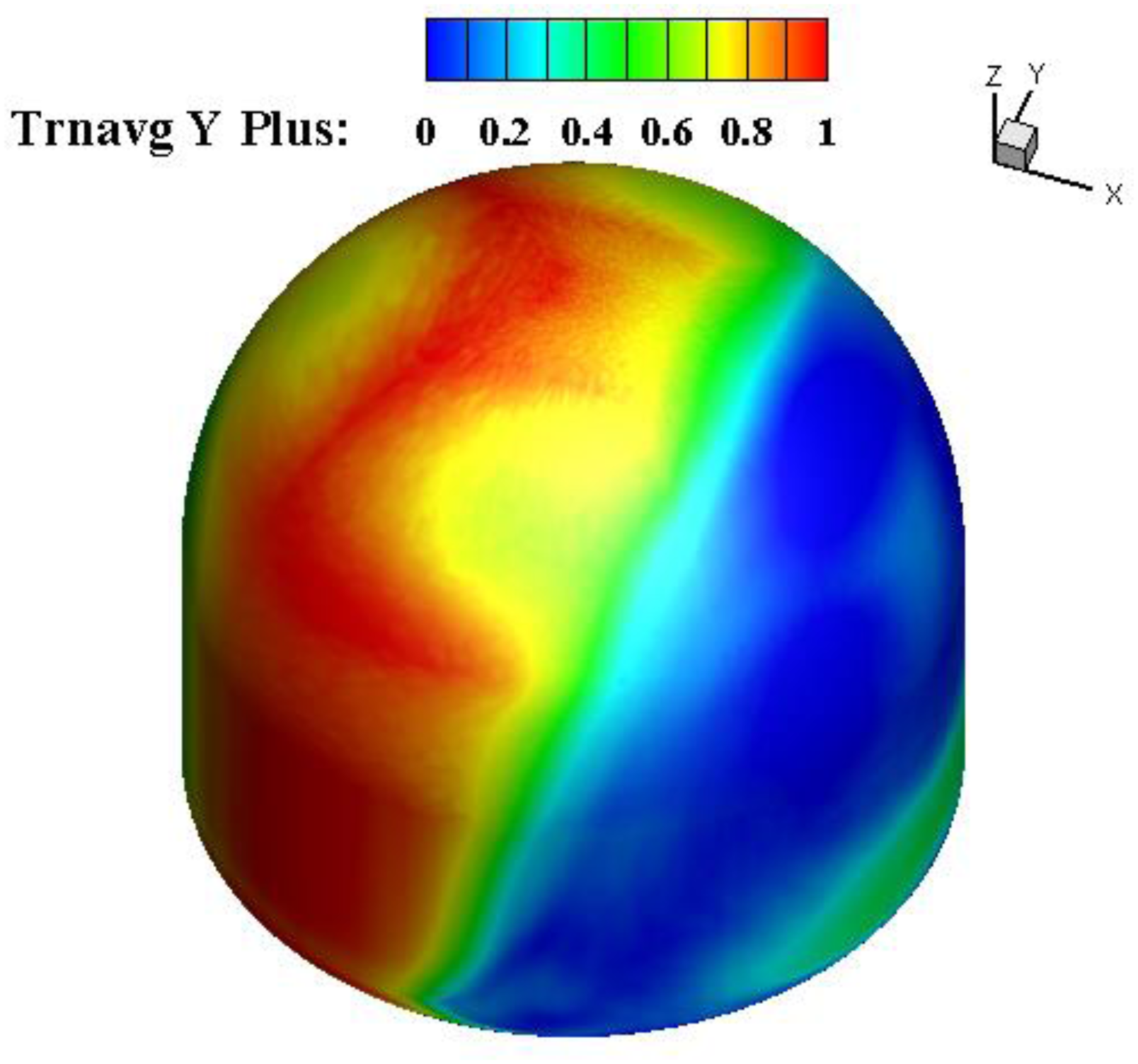
. The spanwise and the height of the computational domain are both 6R. The upstream boundary and downstream boundary are extended to 7.5R and 20R, respectively, to ensure a fully developed turbulent freestream before the turret and fully resolved flow structures in the wake of the turret. The freestream Mach number is Ma = 0.4, which corresponds to a freestream of U_∞ = 138m/s. The temperature and pressure are those under the standard sea-level conditions. The radius of hemisphere is R = 0.1524m and the height of the bottom cylinder is H = 0.1143m. The Reynolds number is Re = 1.43×10⁶, calculated by U_∞ and R. In order to accurately resolve the fluctuant turbulent structures in the wake of turret, the compressible effects and the idea gas model are also taken into account. The inflow is confined by the uniform total pressure boundary condition targeting the U_∞ = 138m/s. The outflow is specified by the static pressure condition which is equal to 1 atm. The no-slip wall condition is set for the surface of the turret and the bottom wall. Notably, it would be better to treat the two-side and top walls as the inviscid wall boundary condition, which means the boundary layers are not resolved on these three walls. In addition, the defaulted adiabatic condition is set for all wall boundaries (the top, side, and bottom walls).

Two sets of structured grids, the coarse and the fine, are generated for the simulation and the grid sensitivity verification. The number of the fine grid is 14 million and the number of the coarse grid is 5 million, shown in Figures 3 and 4. Both grids have the same first-layer height (FLH), which is about 3×10⁻⁶, to ensure y⁺≤1, as shown in Figure 5.

Figure 3.

Grids on the surface of the turret.

Figure 4.

Grids in the X-Z plane with Y = 0.

Figure 5.

y⁺ iso-contour on the turret.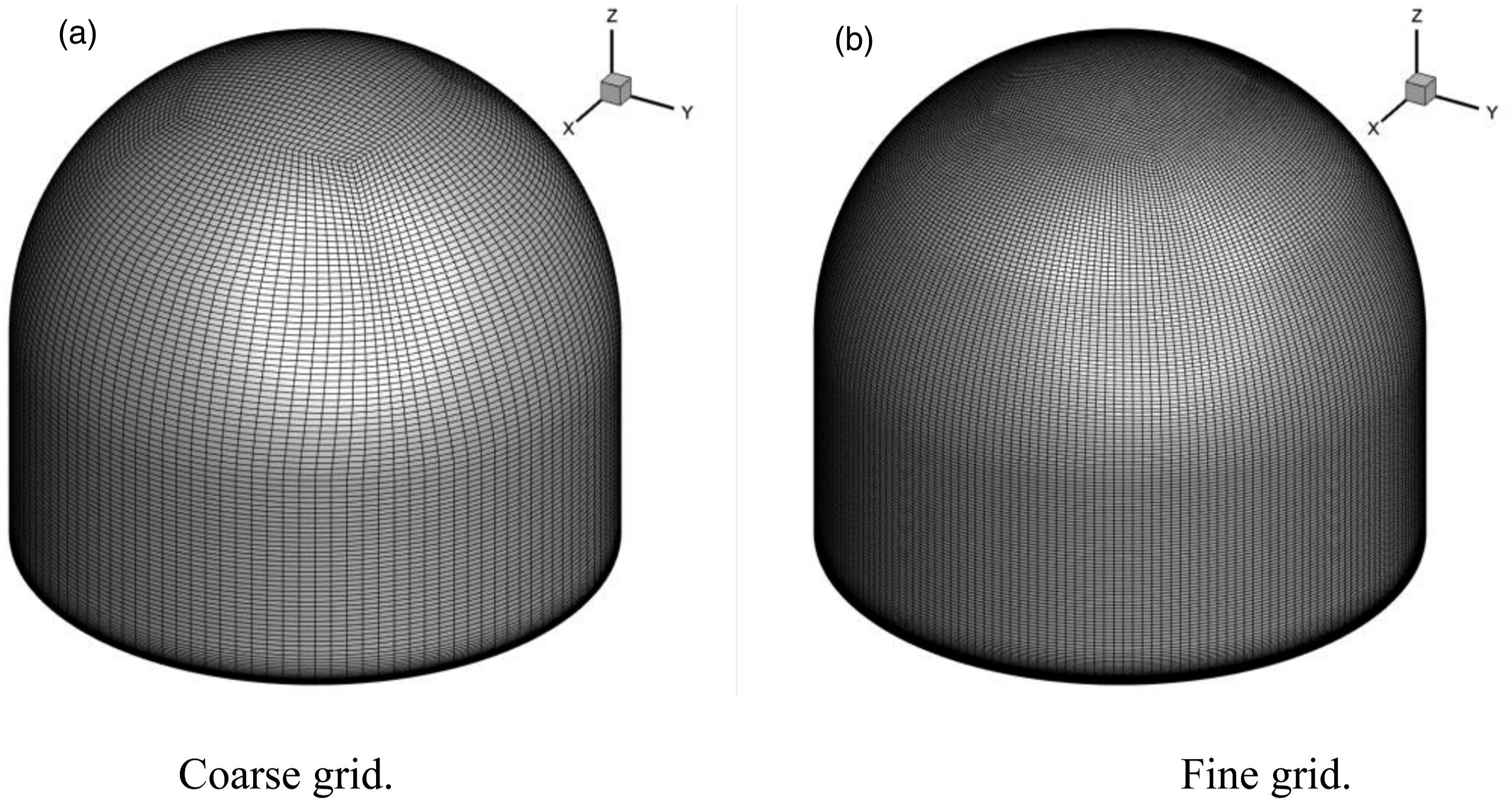

Ray-tracing method

The index of refraction is related to density field based on the Gladstone–Dale relation ¹

$n=1+K_{GD}·\rho ,$

(8)

where n and ρ are the index of refraction and density, respectively; K _GD is the Gladstone–Dale constant, which is usually equal to 2.27×10⁻⁴m³/kg. The integral of the refractive index along the beam path is defined as the optical path length (OPL)

$OPL\left(x^{\prime },y^{\prime },z^{\prime }\right)={\int }_0^{L}n\left(x^{\prime },y^{\prime },z^{\prime }\right)d{z}^{\prime },$

(9)

where x′ and y′ are optical coordinates in the optical window and z′ is along the light propagating direction. Then, the wavefront distortion quantified by the relative difference in the OPL is the optical path difference (OPD), defined as follow:

$OPD\left(x^{\prime },y^{\prime }\right)=OPL\left(x^{\prime },y^{\prime }\right)-〈OPL\left(x^{\prime },y^{\prime }\right)〉,$

(10)

where the angle brackets denote the planar average. Besides, the RMS of the OPD (OPD_rms) is also employed to quantify the wavefront distortion.

Considering the deflection of rays in the flow field, the real path of ray is not a straight line. It is necessary to use ray equation to solve the real path of ray. Based on the ray approximation of the wave equation, beam propagation in a variable density medium follows the following rule:

$\frac{d}{ds}\left[n\left(r\right)\frac{dr}{ds}\right]=\nabla n\left(r\right).$

(11)

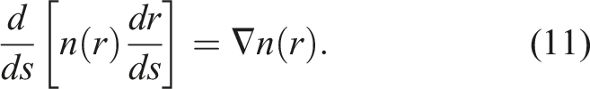
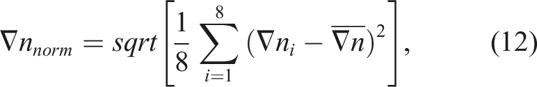
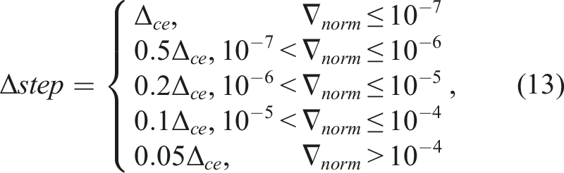
The fourth-order Runge–Kutta method ³⁷ is implemented to trace the rays. The ray-tracing results are determined by the gradient of the index of refraction. In order to improve the accuracy of results and reduce the computational time, the adaptive tracing step is used to solve equation (11), which can make the steps smaller in large gradient regions and make the steps larger in small gradient regions. The normalized gradient of refraction index is shown as follow:

$\nabla n_{norm}=sqrt\left[\frac{1}{8}{\displaystyle \sum }_{i=1}^8{\left(\nabla n_i-\overline{\nabla n}\right)}^2\right],$

(12)

where $\overline{\nabla n}$ is the average gradient of eight vertices of a cell. The tracing step can be constructed as

$\mathrm{\Delta }step=\{\begin{array}{l}{\mathrm{\Delta }}_{ce},{\nabla }_{norm}\le {10}^{-7}\\ 0.5{\mathrm{\Delta }}_{ce},{10}^{-7}<{\nabla }_{norm}\le {10}^{-6}\\ 0.2{\mathrm{\Delta }}_{ce},{10}^{-6}<{\nabla }_{norm}\le {10}^{-5}\\ 0.1{\mathrm{\Delta }}_{ce},{10}^{-5}<{\nabla }_{norm}\le {10}^{-4}\\ 0.05{\mathrm{\Delta }}_{ce},{\nabla }_{norm}>{10}^{-4}\end{array},$

(13)

where ∆ _ce is the mean length scale in the i, j, k directions.

${\mathrm{\Delta }}_{ce}=\left({\mathrm{\Delta }}_i\times {\mathrm{\Delta }}_j\times {\mathrm{\Delta }}_k\right),$

(14)

where ∆ _i , ∆ _j , ∆ _k are the length scale in the i, j, k directions, respectively.

In order to verify the accuracy of the ray-tracing method, a special medium is implemented to ensure the ability of ray tracing for heavily deflected laser beam transmission. The index of refraction can be expressed as follows:

$n^2\left(x,y\right)={n_0}^2\left[1-k^2\left(x^2+y^2\right)\right],$

(15)

where n ₀ and k are the focusing coefficient. The laser beam transmission in the above medium has an analytical solution, which can be expressed as

$\{\begin{array}{l}x=x_0\cos \left(\frac{n_{0}kz}{{\alpha }_0}\right)+\frac{{\beta }_0}{n_{0}k}\sin \left(\frac{n_{0}kz}{{\alpha }_0}\right)\\ y=y_0\cos \left(\frac{n_{0}kz}{{\alpha }_0}\right)+\frac{{\gamma }_0}{n_{0}k}\sin \left(\frac{n_{0}kz}{{\alpha }_0}\right)\end{array},$

(16)

where x₀, y₀, z₀ are the initial position of the laser beam, and x, y, z are the coordinates of the laser beam; α₀, β₀, γ₀ are the products of the refractive index of the initial position and the cosine of the angle between the laser beam direction and x, y, z axis, respectively. Presetting $x_0={\gamma }_0/n_0$ , ${\beta }_0=0$ , the laser beam path satisfies the spiral distribution, which can be described as

$\{\begin{array}{l}x=x_0\cos \left(\frac{n_{0}kz}{{\alpha }_0}\right)\\ y=\frac{{\gamma }_0}{n_{0}k}\sin \left(\frac{n_{0}kz}{{\alpha }_0}\right)\end{array}.$

(17)

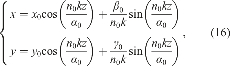
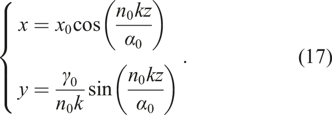
Given the initial condition n₀ = 1.5, k = 0.01, the numerical ray-tracing result and the analytical solution are both shown in Figure 6. The comparison of results indicates that the ray-tracing path perfectly matches with the analytical path. The ray-tracing method meets the precision requirement of aero-optical investigation.

Figure 6.

The index of refraction n on the X-Y plane and the comparison between actual path and ray-tracing path.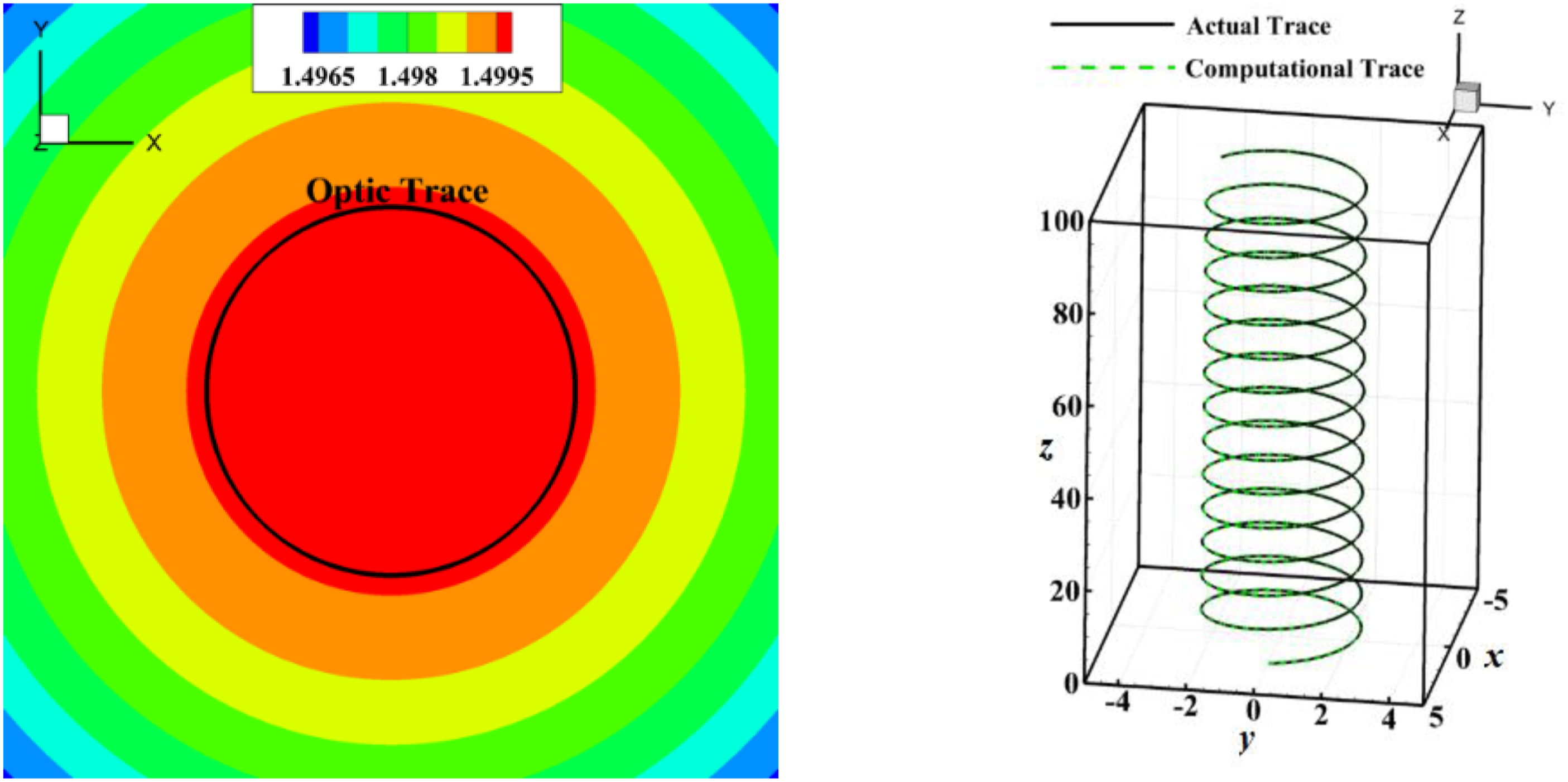

Zernike fitting

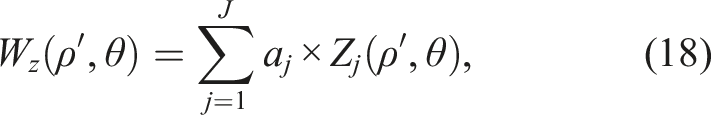
Wavefront distortion refers to the difference between the actual and ideal wavefronts, which can be described by a series of linear combinations of polynomials, namely, Zernike polynomials.^31,32 Each term of the Zernike polynomial has a clear physical meaning and is orthogonal to each other in the unit circle. Thus, the descriptions of Zernike polynomials are performed in polar coordinates. Applying the J-th order polynomial to describe the wavefront distortion ( $W_z\left({\rho }^{\prime },\theta \right)$ ), it can be expressed as follows:

$W_z\left({\rho }^{\prime },\theta \right)={\displaystyle \sum }_{j=1}^J{a}_j\times Z_j\left({\rho }^{\prime },\theta \right),$

(18)

where ρ’ and θ are the polar radius and the polar angle, respectively; a_j is the coefficient of the J-th order Zernike polynomial. The first six items of Zernike polynomial are piston, X/Y tilts, defocus, and X/Y primary astigmatisms. Detailed instruction about the Zernike polynomial can be found in the books written by Zhang et al. ³¹ and Tyson et al. ³² A Zernike polynomial with 36 terms is currently applied to fit wavefront distortion OPD. Therefore, the OPD can be expressed as

$OPD={\displaystyle \sum }_{j=1}^{36}{a}_j\times Z_j\left({\rho }^{\prime },\theta \right).$

(19)

Besides, OPD′, OPD″, and OPD‴ are also used in the present work, which are defined as follows:

$OPD={\displaystyle \sum }_{j=4}^{36}{a}_j\times Z_j\left({\rho }^{\prime },\theta \right),$

(20)

$OPD={\displaystyle \sum }_{j=5}^{36}{a}_j\times Z_j\left({\rho }^{\prime },\theta \right),$

(21)

$OPD={\displaystyle \sum }_{j=7}^{36}{a}_j\times Z_j\left({\rho }^{\prime },\theta \right),$

(22)

Figure 7 shows a given OPD and its counterpart after Zernike polynomial fitting. The result indicates that the difference between the root-mean-square (RMS) of the two OPDs descends to the order of 10⁻¹⁰.

Figure 7.

Contour of the original OPD(left) and the OPD with the Zernike polynomial fitting(right).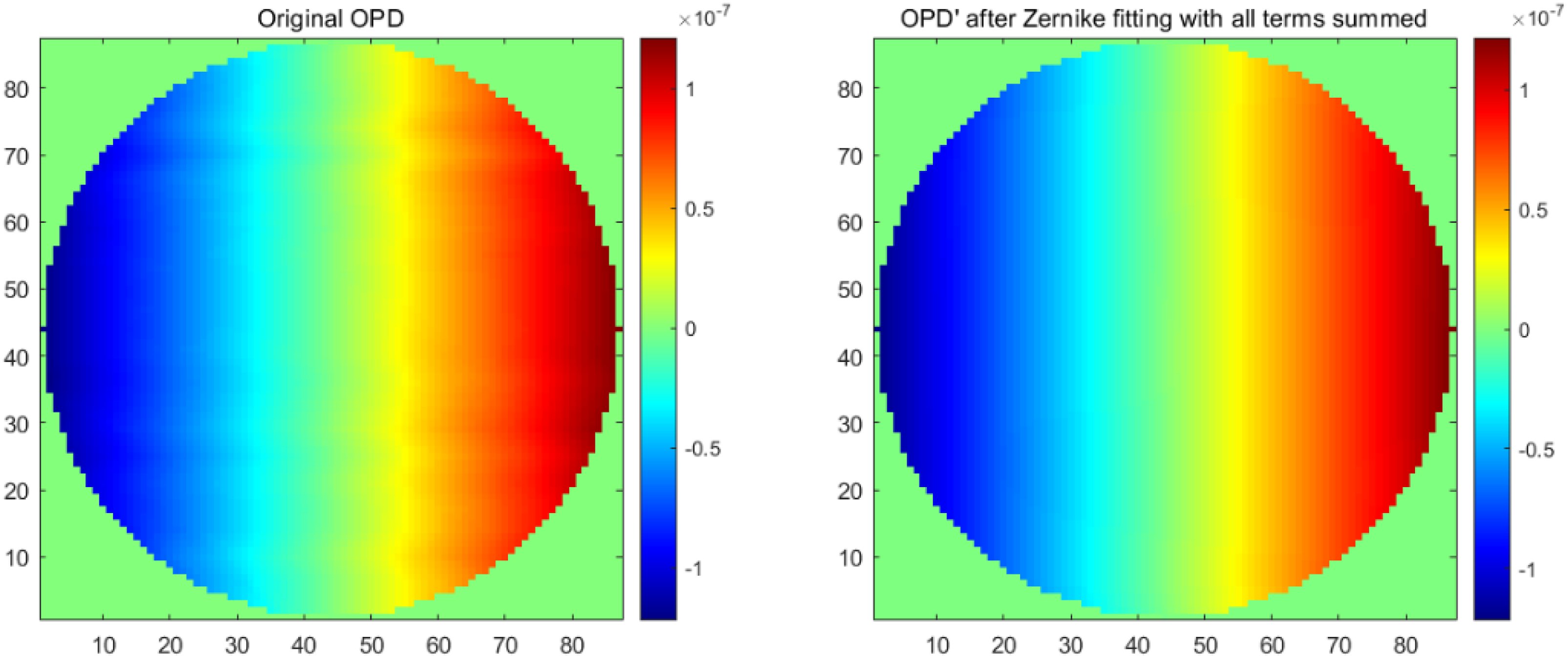

In order to clearly describe the wavefront distortion, the root-mean-square of OPD, OPD′, OPD″, and OPD‴ ( ${OPD}_{rms}$ , ${OPD}_{rms}^{\prime }$ , ${OPD}_{rms}^{″}$ , and ${OPD}_{rms}^{‴}$ ) are also analyzed in this paper.

Results and discussion

Effect of grid resolution

The validation of grid sensitivity investigation for DDES is shown in Figures 8 and 9. Figure 8 presents the comparison of the time-averaged pressure coefficient on the top of the turret between the coarse and the fine grid results. The experimental data in Figure 8 is obtained from the wind tunnel test. ¹¹ The fine grid performs better than the coarse grid in the separation region. The time-averaged pressure coefficient resolved by fine grid is in remarkable agreement with the experimental value. The URANS result with fine grid is similar to the DDES result with coarse grid. This indicates that the DDES can remarkably reduce the grid number under the condition of maintaining the same solution precision.

Figure 8.

Time-averaged pressure coefficient on the top of the turret at the Y = 0 plane.

Figure 9.

Comparison of the distribution of the Y vorticity and the Z vorticity resolved by the fine grid and the coarse grid.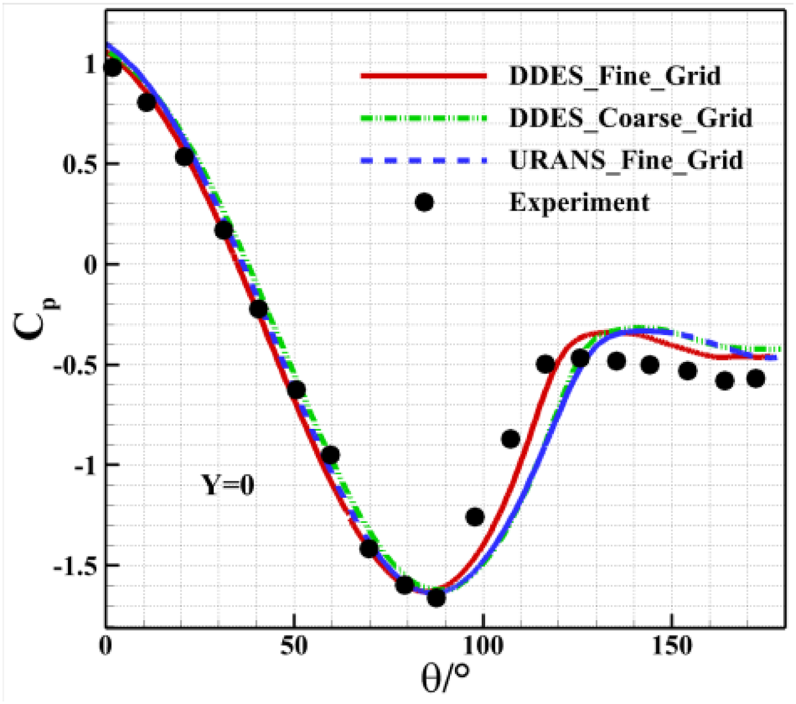

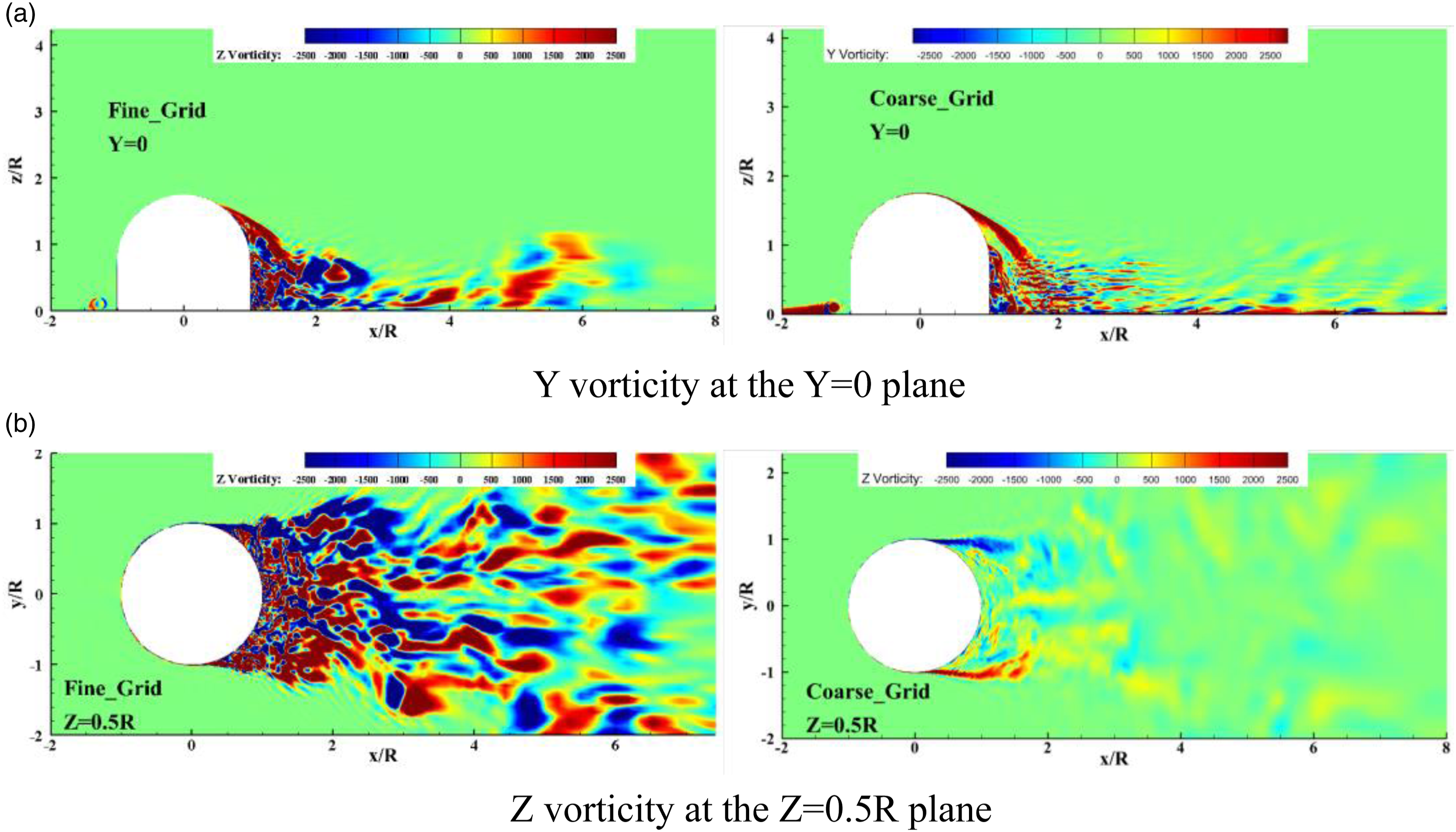
As plotted in Figure 9, the results resolved by the fine grid displays abundant vorticity structures in the wake of the turret. The vorticity distribution is blurry in the results of the coarse grid. The results indicate that the refined grid has a great influence on the separated flow field, but a negligible impact on the attached flow region. Hence, the fine grid is used in the subsequent investigation.

The parallel computation runs in a computer with 14 cores (Intel(R) Xeon(R) CPU E5-2680 v2 @ 2.80GHz), the total time is shown in Table1. The total time includes flow field calculation and optical calculation.

Table 1.

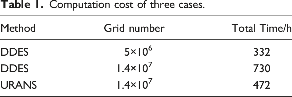
Computation cost of three cases.

Method	Grid number	Total Time/h
DDES	5×106	332
DDES	1.4×107	730
URANS	1.4×107	472

Comparison of flow field resolved by DDES and URANS

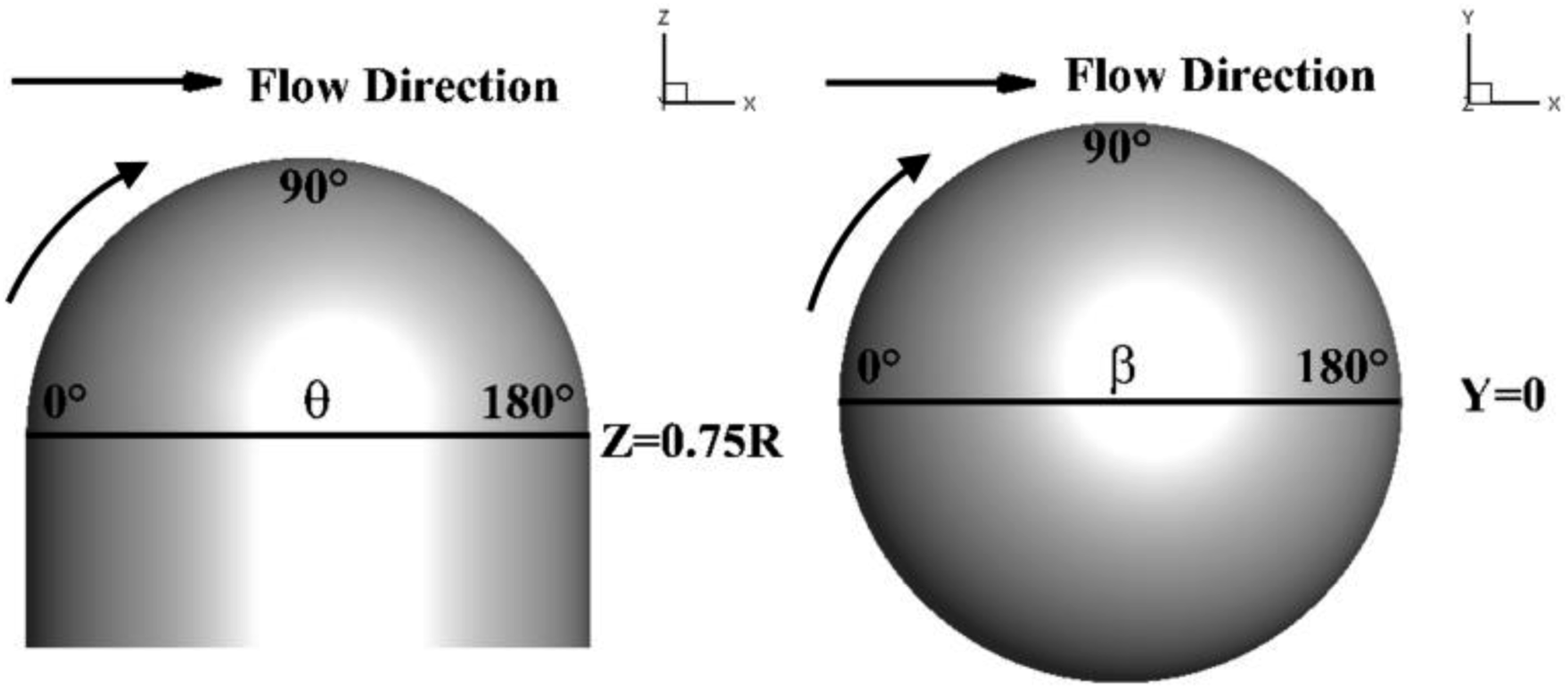
In this section, some typical flow features resolved by DDES and URANS are presented. The performances of DDES and URANS in predicting the separated flow are also discussed in terms of the vorticity structures, spatial flow features, surface flow topology, and turbulence kinetic energy (TKE). Transient flow fields are collected at every 10 iterations in 1000 iterations, which correspond to 0.01s in real time. Some sections are applied to present the flow features. The locations of these sections and the definition of $\theta$ and $\beta$ are shown in Figures 10 and 11, respectively.

Figure 10.

Sections shown in red dashed lines.

Figure 11.

Azimuthal angles θ and β.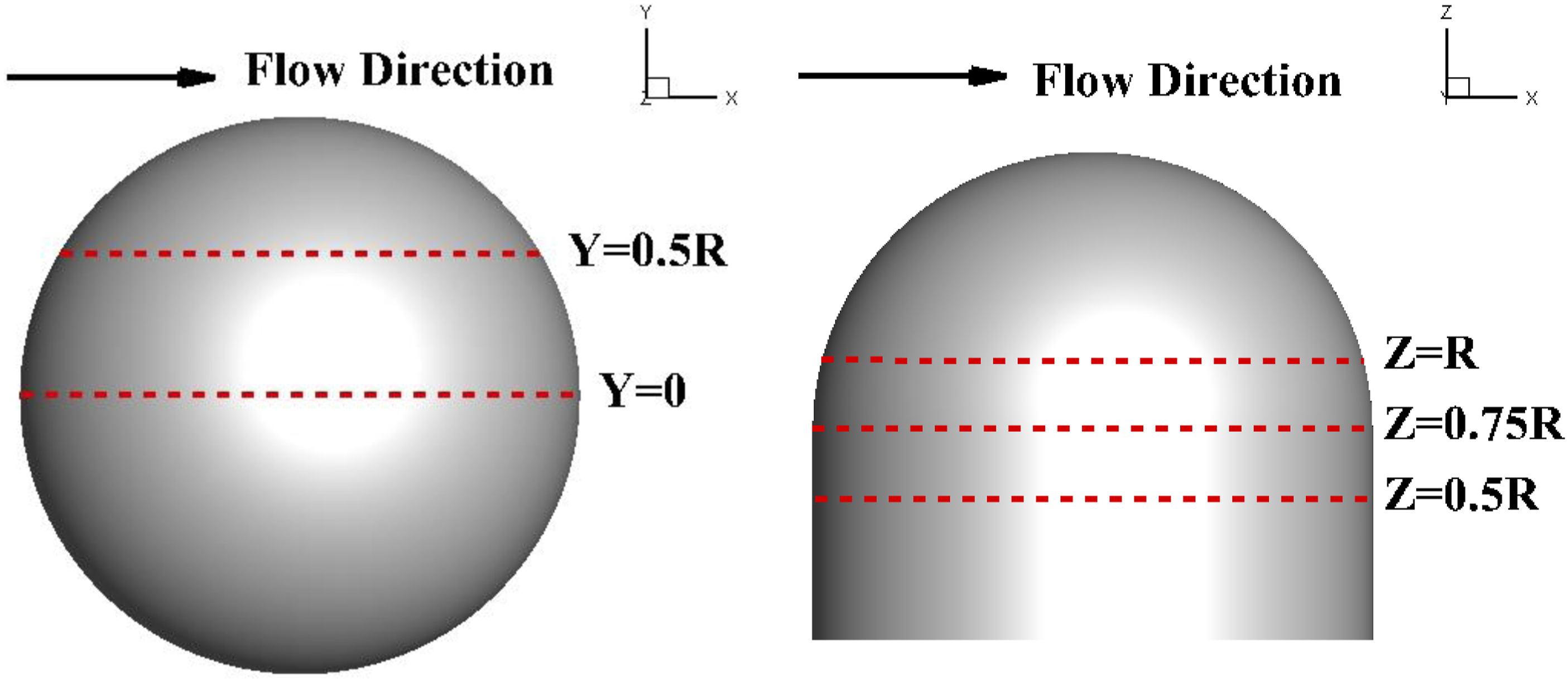

As depicted in Figure 12, instantaneous flow fields are demonstrated by the iso-surface of Q criterion, colored by time-averaged turbulent viscosity ratio. The peak of turbulent viscosity ratio by DDES and URANS are 1061 and 10,325. The simulated results show that DDES can capture abundant small vortical structures and URANS resolves only a few large-scale vortices. Specifically, there are two thin necklace vortices and a thick necklace vortex resolved by DDES and URANS, respectively. This indicates that DDES performs far better than URANS in resolving vortical structures. Notably, the wake flow resolved by URANS shows the higher values of turbulent viscosity ratio. In DDES, the LES mode is used to resolve the separated flow and lots of high-frequency vortices are captured, corresponding to the lower turbulent dissipation. Therefore, the turbulent viscosity ratio of DDES is smaller than that of URANS.

Figure 12.

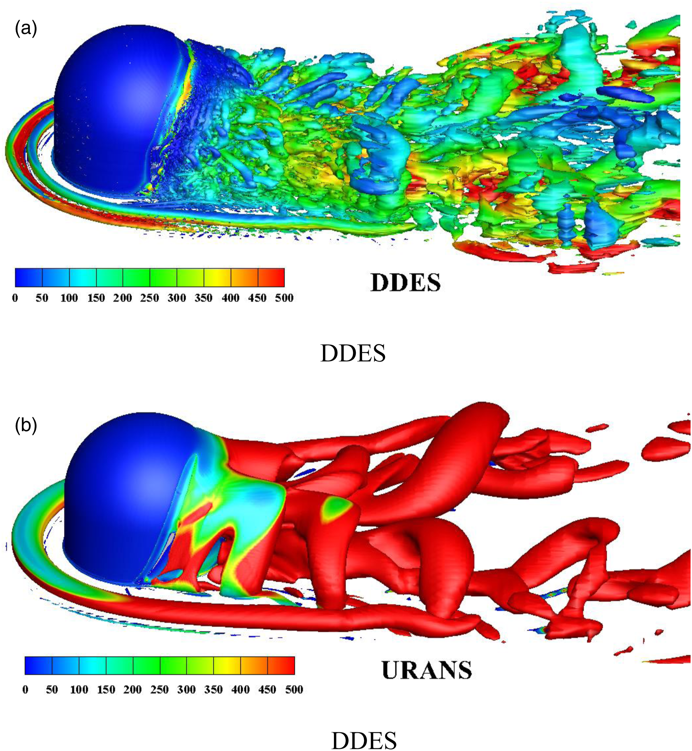
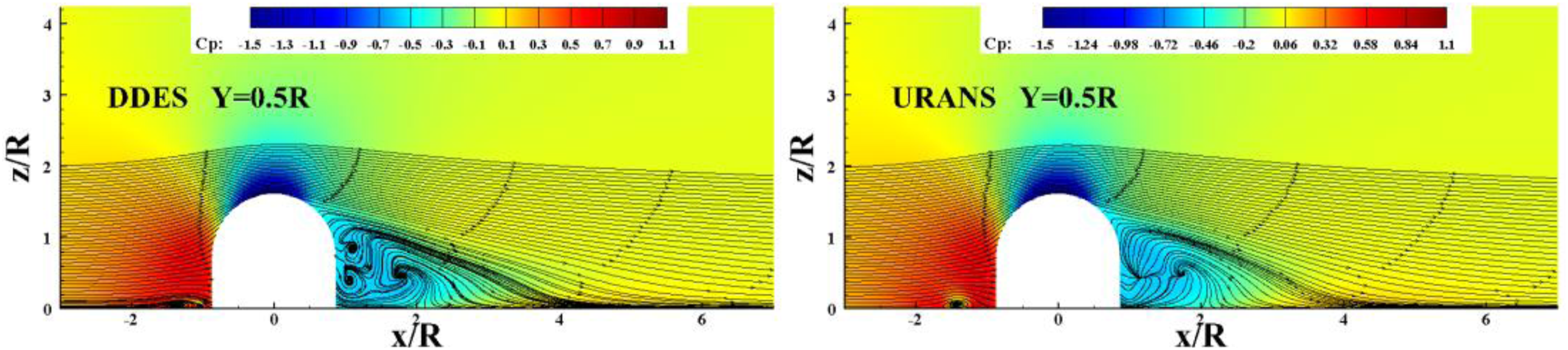
The iso-surface of Q criterion of vorticity of the transient flow fields resolved by DDES and URANS, respectively, colored with the turbulent viscosity ratio ${\mu }_t/\mu$ .

Figures 13 and 14 show the time-averaged flow features at the X-Z plane around the turret simulated by DDES and URANS. The timed-averaged flow fields are generally similar for both methods. Both plots show a back-flow region at the back of the turret. As shown in Figure 13, the plot of DDES appears a separated region at the front and the back of the turret, but the flow phenomenon is not obvious in the URANS result. The similar conclusion is displayed in Figure 14. The contour plotted by DDES shows three remarkable separated regions, but there is only one big separated region in the contour drawn by URANS.

Figure 13.

Time-averaged pressure coefficient with streamlines on the X-Z plane at Y = 0.

Figure 14.

Time-averaged pressure coefficient with streamlines on the X-Z plane at Y = 0.5R.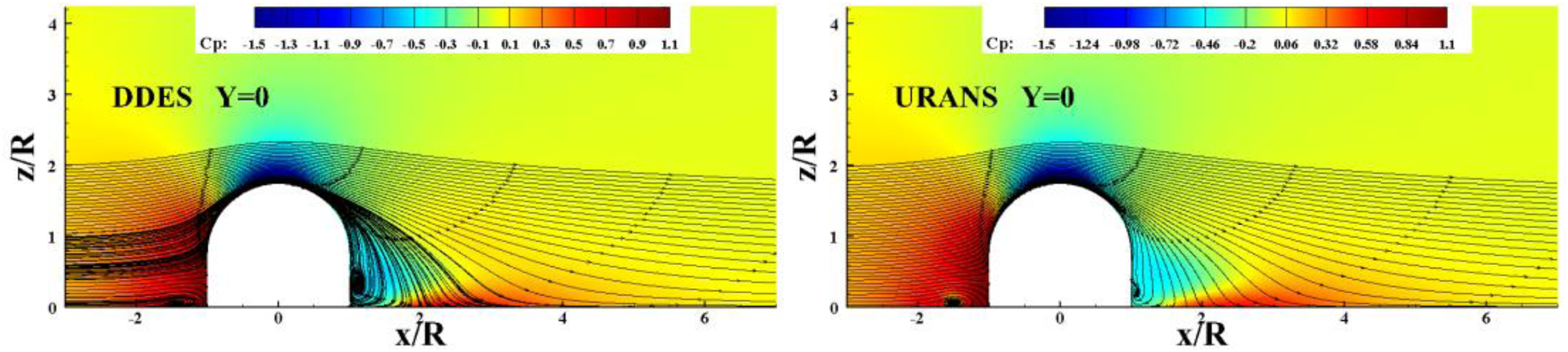

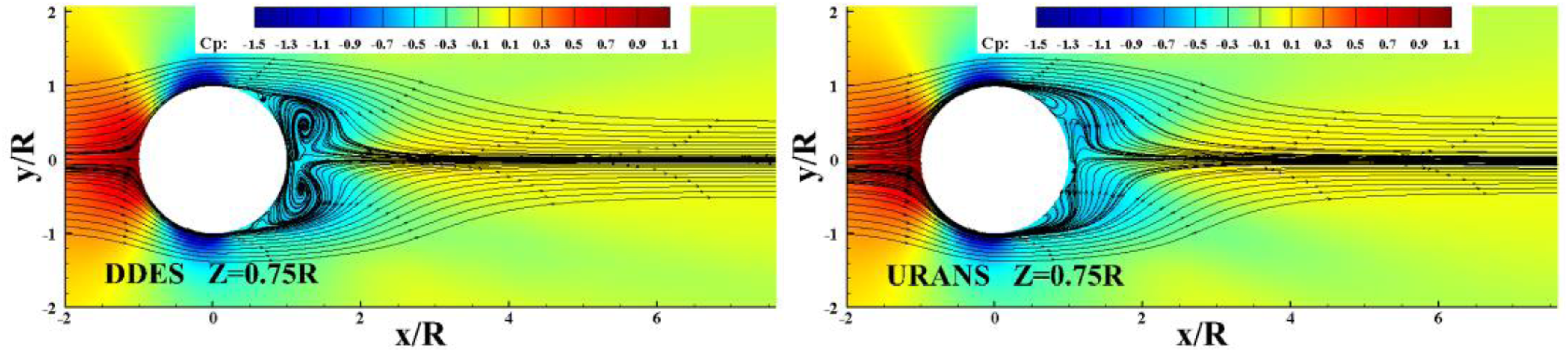
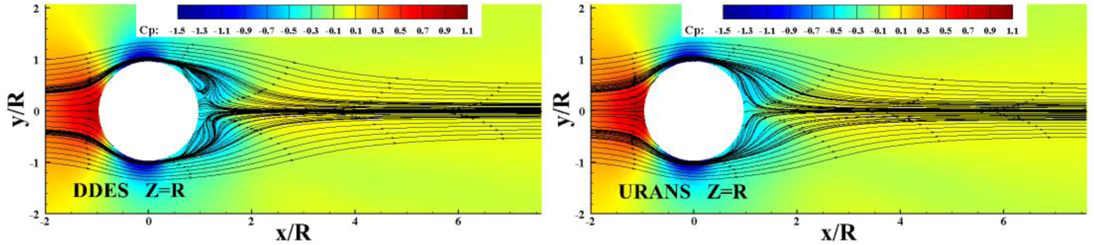
Figures 15, 16, and 17 present the time-averaged flow features at the X-Y plane. The general flow features are also similar for both simulations. Behind the turret, a pair of large and almost symmetrical recirculation zone can be observed, but their shape and extension are different from each other. At the Z = 0.5R section, there are an obvious phenomenon of flow separation as well as reattachment in DDES and URANS. Particularly, several small separation regions are formed in the process of separation as well as reattachment in DDES. At the Z = 0.75R section, the flow of DDES forms a pair of separated regions, and it separates from both sides of the turret and is converged at the symmetric line, which does not reattach to the turret. The flow of URANS shows clear separation as well as reattachment. At the Z = R section, the flow resolved by DDES presents the slight separation at the back of the turret. The flow of URANS only displays the attached flow.

Figure 15.

Time-averaged pressure coefficient with streamlines on the X-Y plane at Z = 0.5R.

Figure 16.

Time-averaged pressure coefficient with streamlines on the X-Y plane at Z = 0.75R.

Figure 17.

Time-averaged pressure coefficient with streamlines on the X-Y plane at Z = R.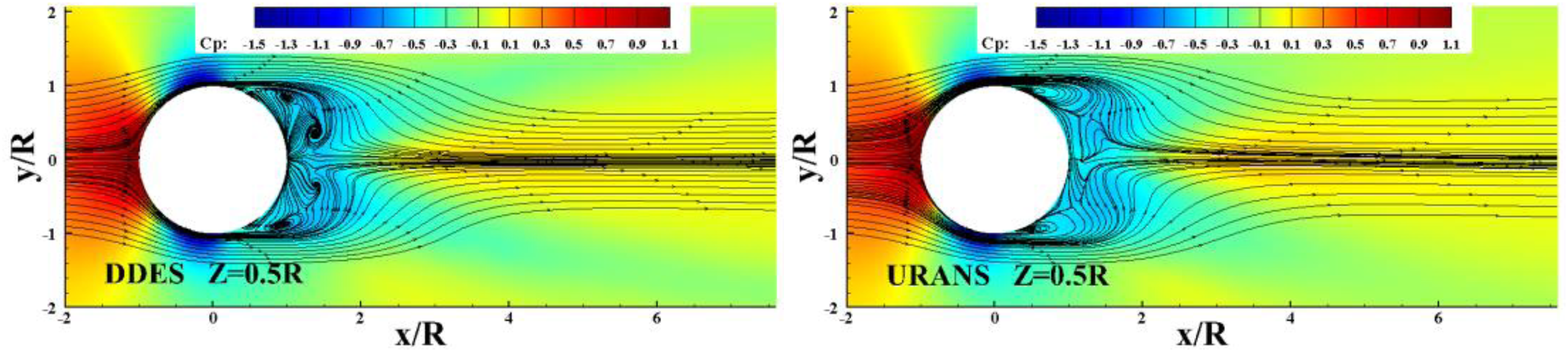

Comparisons of the mean surface streamline between DDES and URANS on the surface of the turret are presented in Figures 18 and 19. The plots are also colored with the time-averaged pressure coefficient. In order to describe the surface flow patterns easily, the critical points theory^38,39 is introduced in this work, as shown in Figure 18. Typical flow topologies include Unstable Node (USN), Stable Node (SN), Unstable Foci (UF), Stable Foci (SF), Bifurcation Line of Attachment (BLA), and Bifurcation Line of Separation (BLS).

Figure 18.

Definition of typical flow topology on the surface.

Figure 19.

Surface streamline and time-averaged pressure coefficient, windward view.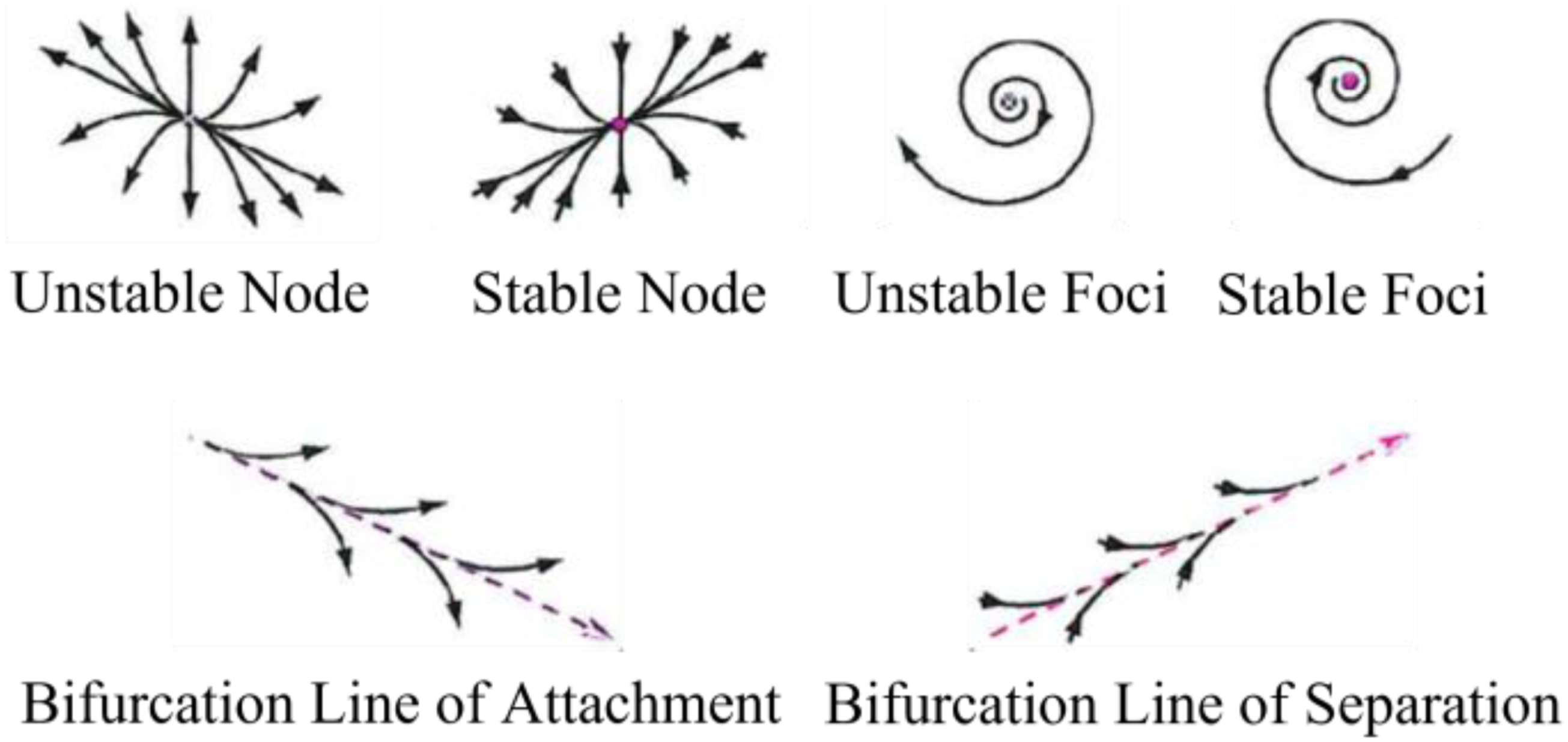

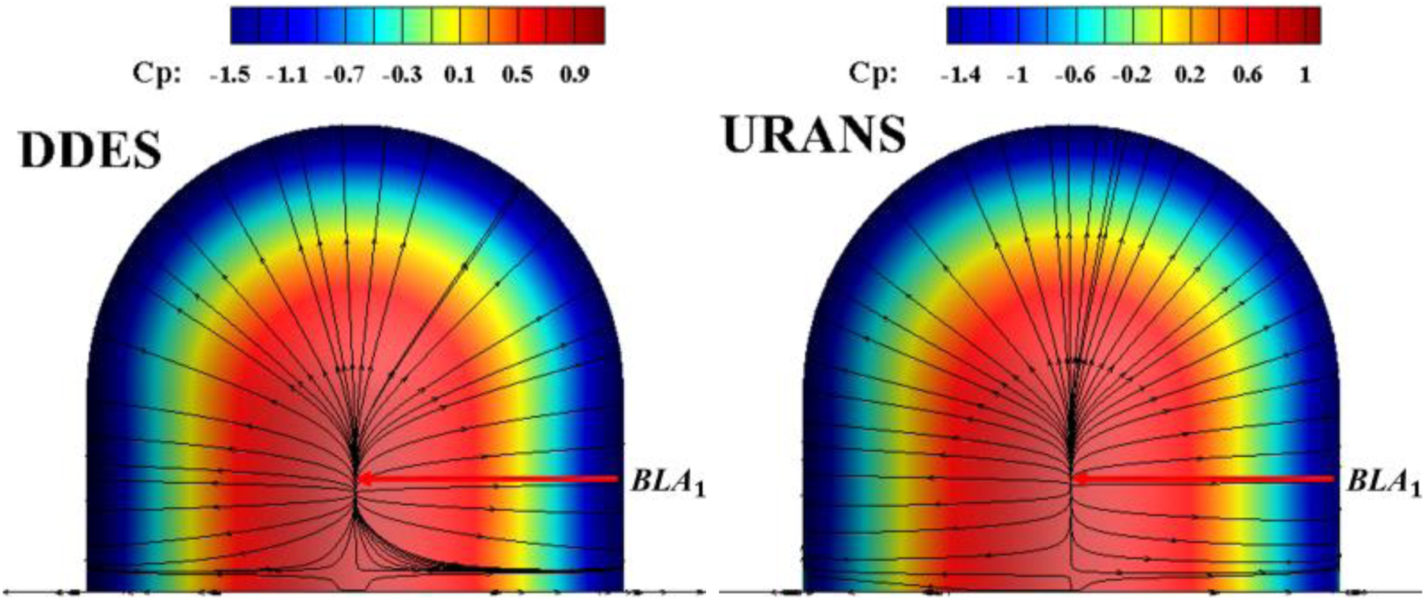
In the windward view, plotted in Figure 19, the surface streamlines and the time-averaged pressure coefficient distribution of both methods are in general agreement, which is because the flow is attached to the turret surface. The high-pressure region is corresponding to the stagnation point BLA₁, which is formed by the impingement of incoming flow with the turret. The BLA₁ is also generally similar for the two methods. In the leeward of the turret, shown in Figure 20, flow patterns are more remarkably complex than those in the windward view. Obviously, the pressure in the leeward is far lower than that in the windward view due to the flow separation. There are two stable focuses (SF₁ and SF₂) formed by the high-speed flow of DDES, but three stable focuses (SF₁, SF₂, and SF₃) are presented in the plot resolved by URANS. The SF leads to the unsteady behaviors like vortex shedding. Both plots in Figure 20 have the similar BLA₂, and the location of the BLA₂ of DDES is slightly higher than that of URANS. The BLA₂ is caused by the impingement of the back flow with the turret and has a big impact on the SF₁, SF₂, and SF₃. Notably, a pair of unstable nodes (USN₁ and USN₂) is presented in the plot of DDES, which is obviously different from the plot of URANS. The USN₁ and the USN₂ might be caused by the separated flow reattachments on the two sides of the turret.

Figure 20.

Surface streamline and time-averaged pressure coefficient, leeward view.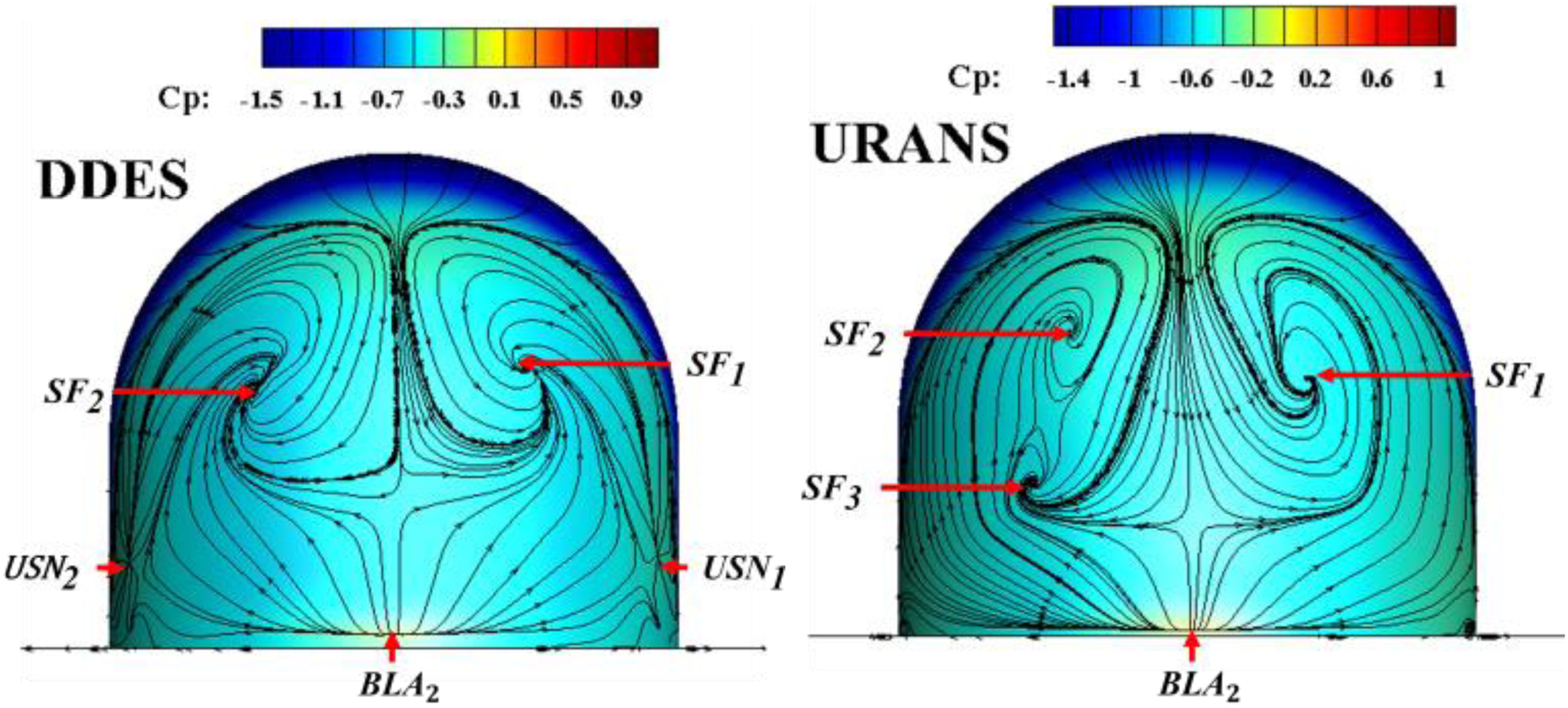

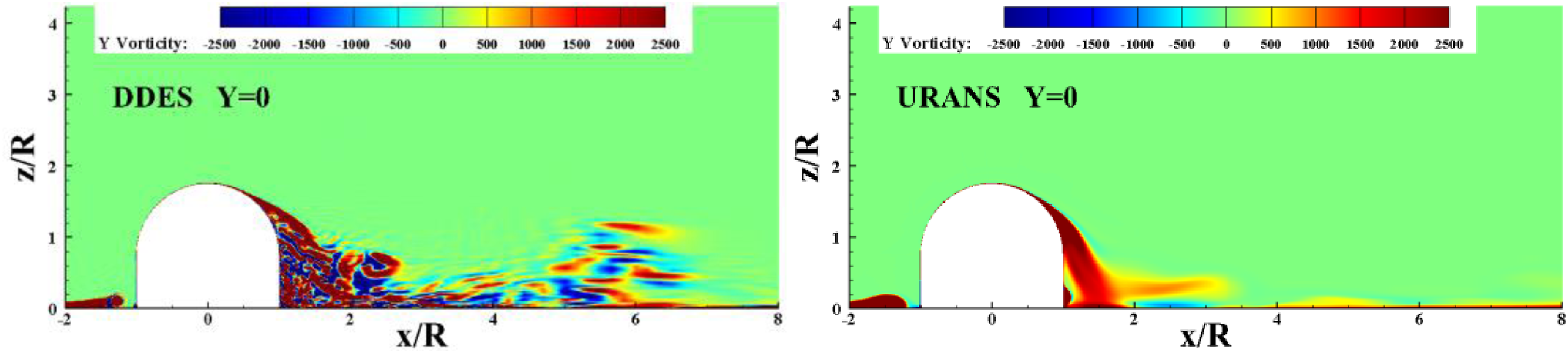
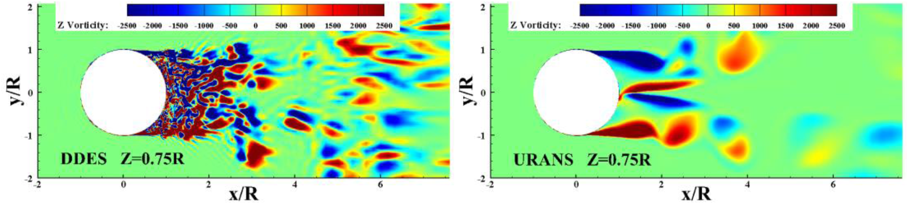
The time-averaged turbulent kinetic energy (TKE) of the two methods is presented in Figures 21 and 22. The results indicate that the TKE of URANS is far higher than that of DDES, which is due to the large vortexes and the higher dissipation of URANS. The time-averaged TKE peaks at values of about 596.2 and 1358 for DDES and URANS, respectively. The DDES can capture more and smaller vortexes, so that the dissipation for DDES is smaller. The results are obviously reflected in Figures 23 and 24.

Figure 21.

Distribution of time-averaged turbulent kinetic energy at Y = 0 section.

Figure 22.

Distribution of time-averaged turbulent kinetic energy at Z = 0.75R section.

Figure 23.

Distribution of vorticity at Y = 0 section.

Figure 24.

Distribution of vorticity at Z = 0.75R section.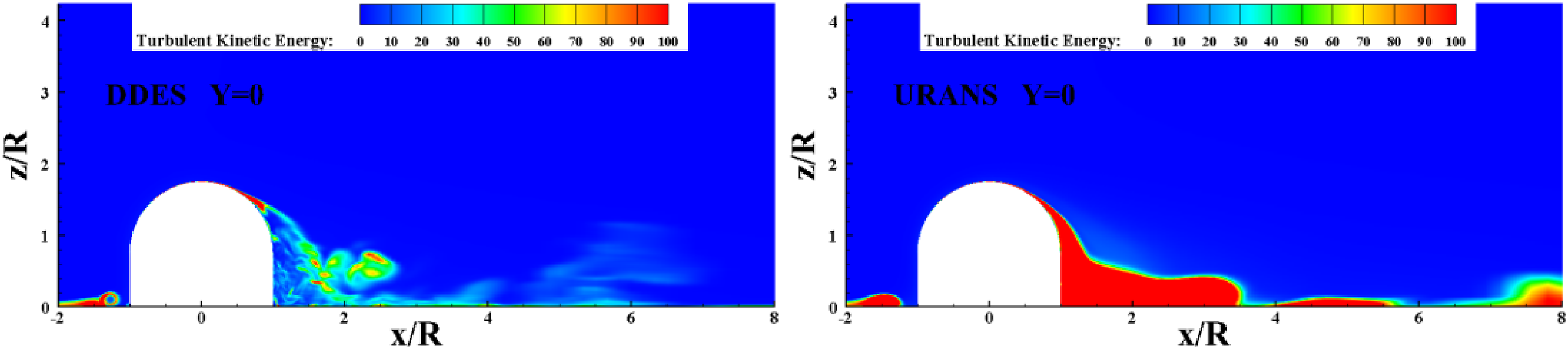

3.3 Aero-optical effects based on DDES and URANS

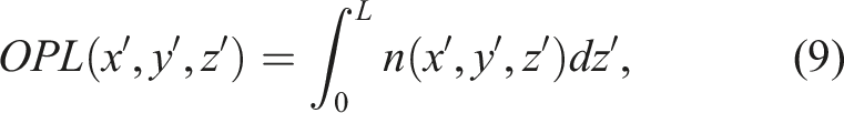
Further investigations on the aero-optical effects are performed using DDES and URANS in the following work. A square aperture with a side length of 0.9R is used for laser beam transmission, plotted in Figure 25. The coordinates of x′, y′, z′ are taken into account for the optical calculation, where the x′ and y′ are on the original optical window and the z′ is normal to the optical plane. The blue rectangle grid with red line represents the optical grid, which is in the size of 0.9R × 0.9R × 4R, corresponding to the x′, y′, z′ coordinates, respectively. The fluctuated densities, resolved by DDES and URANS, are linearly interpolated to the optical grid at each ten time-steps. In order to simulate the light transmission process realistically, the starting position of tracing is set inside the turret.

Figure 25.

Schematics of the relation of optical grid and flow field (left), and the ray-tracing procedure (right).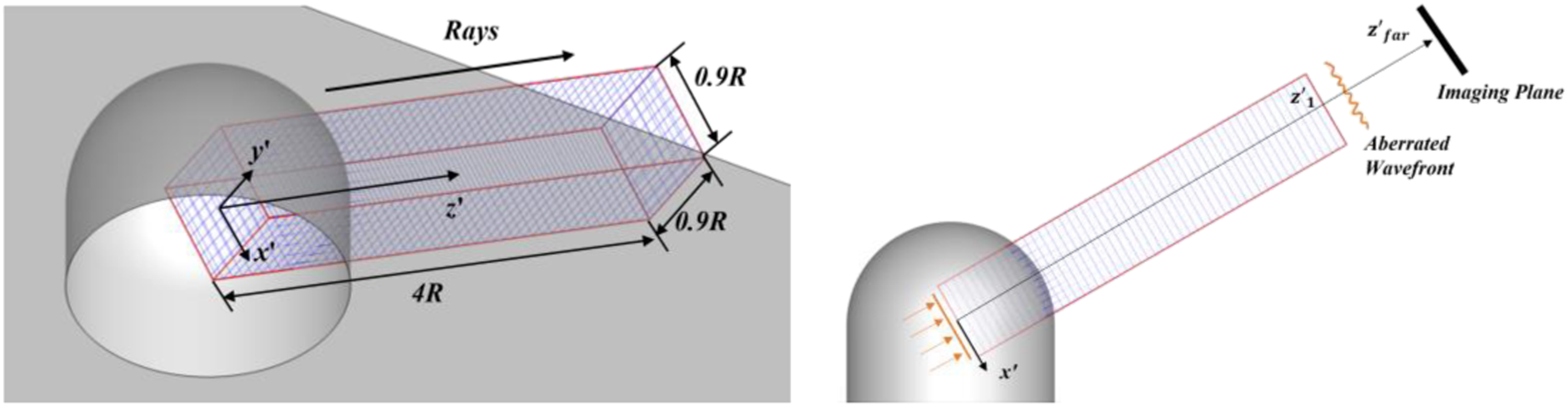

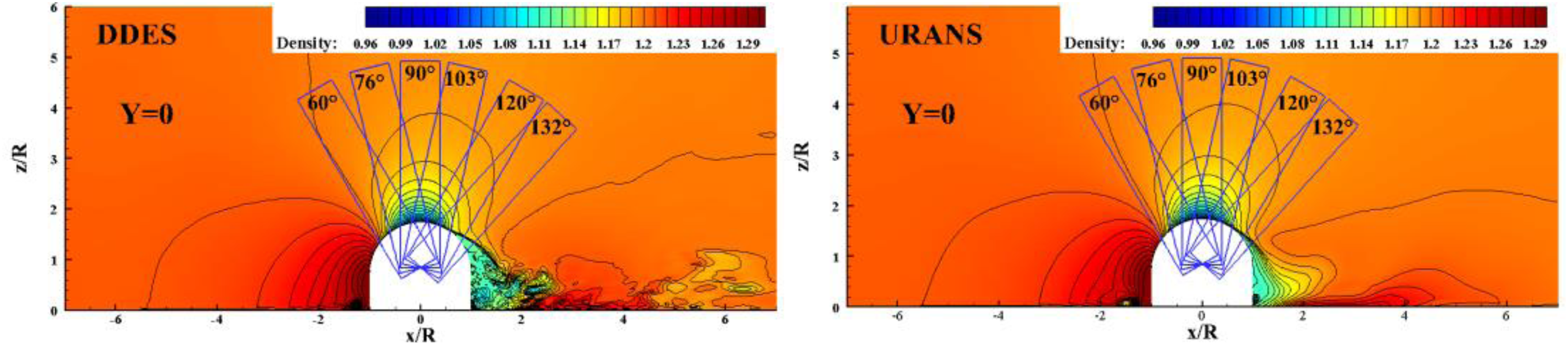
Figure 26 shows the comparison of time-averaged density distribution of DDES and URANS. At three sections, both time-averaged density distributions are generally similar in the region where the laser beam passes through. Slight differences are presented in the region of the elevation angles of 120° and 132°. As plotted in Figure 27, instantaneous density distributions are also presented at three different sections. The results indicate that the instantaneous density distributions are approximately similar in the region of the attached flow, and the density distributions are different in the separated flow region. The fluctuation of instantaneous density distribution of DDES are far greater than that of URANS. This is because that DDES can resolve abundant flow structures in the separated region.

Figure 26.

Distribution of time-averaged density at the three sections (Y = 0), and optical grid are represented by blue rectangles at different angles.

Figure 27.

Distribution of instantaneous density at the three sections (Y = 0), represented by blue rectangles at different angles.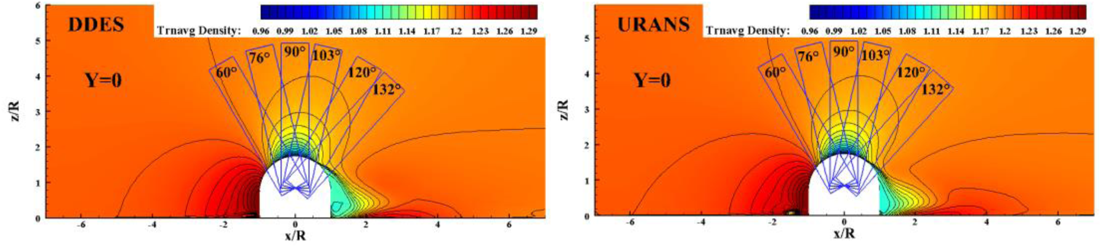

In the present work, the Gladstone–Dale relation is used to calculate the index of refraction. The wavelength is λ = 0.75μm, corresponding to K _GD = 2.27×10⁻⁴m³/kg. Notably, in this work, wavefront distortion are calculated over 100 transient samples of density distribution, which can resolve the influence of turbulent fluctuation on the aero-optical effect.

Figure 28 present the ${OPD}_{rms}^{″}$ and ${OPD}_{rms}^{‴}$ at six different angles of elevation for DDES and URANS. The experimental data in two plots are obtained from the wind-tunnel test by Gordeyev et al. ¹¹ In Gordeyev’s test, three different optical wavefront devices, a Mally probe (Mally), a commercial 2-D wave front sensor (WFS), and a high-bandwidth wavefront sensor (high-bandwidth WFS), were applied to measure the optical aberrations. The influence of spherical optical window was corrected by a concave lens, which was actually to correct the defocus component (the fourth item in the Zernike polynomial). Particularly, in the measurement of the WFS, the tilt components of each instantaneous wavefront were removed, which was actually to correct the piston component and X/Y tilt components (the first three items in the Zernike polynomial). In the measurement of the Mally probe and the high-bandwidth wavefront sensor, the stationary aberrations were removed, corresponding to correction of the piston component, X/Y tilt components, and X/Y primary astigmatism components (the first three items and the fifth and sixth items in the Zernike polynomial). Thus, the optical aberrations measured by WFS are corresponding to ${OPD}_{rms}^{″}$ , and the optical aberrations measured by Mally probe and high-bandwidth WFS are corresponding to ${OPD}_{rms}^{‴}$ .

Figure 28.

Comparison of the simulated results and the experimental results. ¹¹

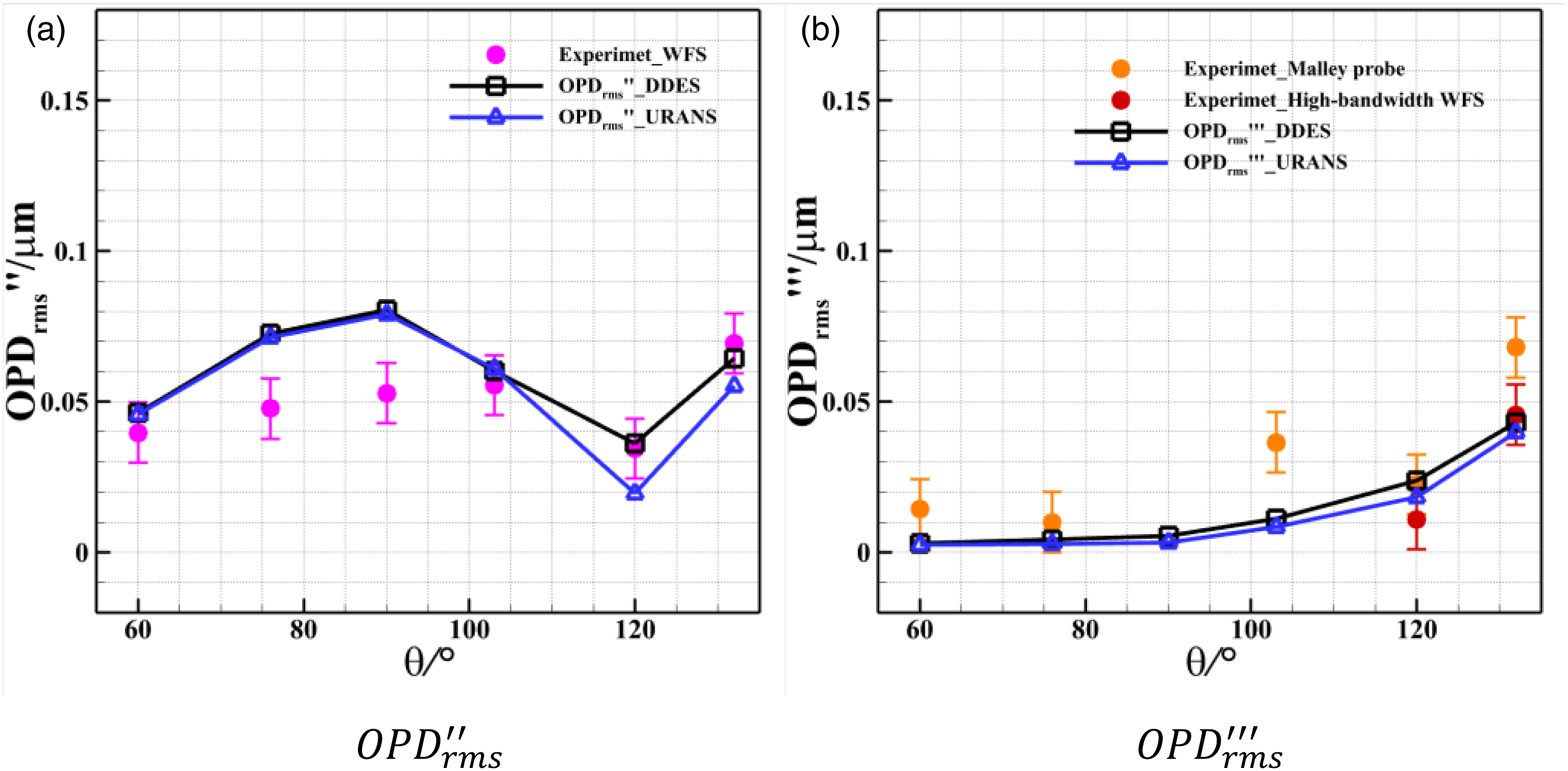
The results show that ${OPD}_{rms}^{″}$ and ${OPD}_{rms}^{‴}$ calculated in this work are in generally good agreement with the experimental data. In Figure 28(a), both DDES and URANS results are slightly larger than the experimental result at angles of 76° and 90°, which is probably because that both DDES and URANS resolve the boundary layer with turbulent solution, whereas in the experiment, these regions are laminar flow. This phenomenon is also found in the study by Morgan et al. ¹⁸ Therefore, the density distribution are more disordered than experiment, and the value of ${OPD}_{rms}^{″}$ is also bigger. At the angles of 60°, 76°, 90°, and 103°, the differences of ${OPD}_{rms}^{″}$ resolved by DDES and URANS are within 1%. At the angles of 120° and 132°, ${OPD}_{rms}^{″}$ of DDES agrees well with the experiment, and the differences of ${OPD}_{rms}^{″}$ resolved by DDES and URANS are 45.7% and 14.5%, respectively. This is due to that DDES can resolve the elaborate instantaneous density distribution in separated regions, and the index of refraction of DDES is more accurate than that of URANS, as shown in Figure 28. In Figure 28(b), ${OPD}_{rms}^{‴}$ of DDES is higher than that of URANS. At the six angles, the difference of ${OPD}_{rms}^{‴}$ resolved by two methods are 12%, 35.9%, 42.5%, 24.4%, 22.4%, and 6.9%, respectively. Although the percentage of two methods are a bit large, the absolute differences of results by two methods are remarkably small. The maximal absolute differences of ${OPD}_{rms}^{″}$ and ${OPD}_{rms}^{‴}$ are at the angle of 120°, whose values are only 0.0165μm and 0.0053μm, respectively. In addition, both simulated results are also within the error margin of the experiment data.

Tables 2, 3, 4, 5, 6, and 7 show the value of the time-averaged ${OPD}_{rms}$ , ${OPD}_{rms}^{\prime }$ , ${OPD}_{rms}^{″}$ , and ${OPD}_{rms}^{‴}$ of DDES and URANS at five different tracing distances, z’=0.3R, 0.9R, 1.8R, 2.7R, and 3.6R, at six angles of elevation. At the angles of 60°, 76°, 90°, and 103°, ${OPD}_{rms}$ , ${OPD}_{rms}^{\prime }$ , ${OPD}_{rms}^{″}$ , and ${OPD}_{rms}^{‴}$ of DDES and URANS are generally similar at every tracing distance, presented in Figure 29. The specific value differences of two methods are shown in Tables 2, 3, 4, and 5. At these four angles of elevation, the laser beam passes through the attached turbulent boundary layer, and the turbulent fluctuations are very gentle. The fluctuations of density distribution in these regions are also very weak, plotted in Figure 27. The abilities of resolving the attached flow for DDES and URANS are generally equal. However, when the laser beam passes through the separated flow region, the optical distortions for DDES and URANS are remarkably different. The variation tendency of ${OPD}_{rms}$ , ${OPD}_{rms}^{\prime }$ , ${OPD}_{rms}^{″}$ , and ${OPD}_{rms}^{‴}$ at different tracing distances are similar, but the differences of their values are obvious. At the angles of 120° and 132°, the value of ${OPD}_{rms}$ of DDES is smaller than that of URANS, and the values of ${OPD}_{rms}^{\prime }$ , ${OPD}_{rms}^{″}$ , and ${OPD}_{rms}^{‴}$ of DDES are bigger than that of URANS. This is because that URANS resolves large and stationary flow vortexes, and these structures mainly influence the X/Y tilts components in wavefront distortion. Therefore, the value of ${OPD}_{rms}$ of URANS is bigger. When the tilt components are removed, the influences caused by large flow structures are eliminated. DDES can resolve abundant and unstable flow structures, which have a great impact on wavefront distortion. Thus, after removing first three items in the Zernike polynomial, ${OPD}_{rms}^{\prime }$ , ${OPD}_{rms}^{″}$ , and ${OPD}_{rms}^{‴}$ of DDES are always bigger than that of URANS at the different tracing distances.

Table 2.

Time-averaged ${OPD}_{rms}$ , ${OPD}_{rms}^{\prime }$ , ${OPD}_{rms}^{″}$ , and ${OPD}_{rms}^{‴}$ at five different tracing distances of DDES and URANS at the elevation of 60°.

	DDES				URANS
Dis	${OPD}_{rms}$	${OPD}_{rms}^{\prime }$	${OPD}_{rms}^{″}$	${OPD}_{rms}^{‴}$	${OPD}_{rms}$	${OPD}_{rms}^{\prime }$	${OPD}_{rms}^{″}$	${OPD}_{rms}^{‴}$
0.3R	0	0	0	0	0	0	0	0
0.9R	0.07228	0.07263	0.05399	0.05372	0.07281	0.07347	0.05510	0.05485
1.8R	0.46838	0.04330	0.04239	0.00533	0.47694	0.04309	0.04227	0.00507
2.7R	0.55296	0.04593	0.04541	0.00306	0.56283	0.04568	0.04525	0.00271
3.6R	0.58523	0.04653	0.04604	0.00292	0.59602	0.04528	0.04590	0.00250

Table 3.

Time-averaged ${OPD}_{rms}$ , ${OPD}_{rms}^{\prime }$ , ${OPD}_{rms}^{″}$ , and ${OPD}_{rms}^{‴}$ at five different tracing distances of DDES and URANS at the elevation of 76°.

	DDES				URANS
Dis	${OPD}_{rms}$	${OPD}_{rms}^{\prime }$	${OPD}_{rms}^{″}$	${OPD}_{rms}^{‴}$	${OPD}_{rms}$	${OPD}_{rms}^{\prime }$	${OPD}_{rms}^{″}$	${OPD}_{rms}^{‴}$
0.3R	0	0	0	0	0	0	0	0
0.9R	0.08714	0.07774	0.03215	0.03115	0.08838	0.07904	0.03352	0.03259
1.8R	0.27622	0.06686	0.06562	0.00341	0.28462	0.06589	0.06467	0.002715
2.7R	0.33361	0.07379	0.07109	0.00392	0.34293	0.07291	0.07017	0.00250
3.6R	0.35811	0.07537	0.07234	0.00417	0.36781	0.07453	0.07144	0.00267

Table 4.

Time-averaged ${OPD}_{rms}$ , ${OPD}_{rms}^{\prime }$ , ${OPD}_{rms}^{″}$ , and ${OPD}_{rms}^{‴}$ at five different tracing distances of DDES and URANS at the elevation of 90°.

	DDES				URANS
Dis	${OPD}_{rms}$	${OPD}_{rms}^{\prime }$	${OPD}_{rms}^{″}$	${OPD}_{rms}^{‴}$	${OPD}_{rms}$	${OPD}_{rms}^{\prime }$	${OPD}_{rms}^{″}$	${OPD}_{rms}^{‴}$
0.3R	0	0	0	0	0	0	0	0
0.9R	0.09124	0.07908	0.01439	0.01122	0.09349	0.08075	0.01367	0.01053
1.8R	0.07752	0.07543	0.07260	0.00496	0.07549	0.07388	0.07124	0.00312
2.7R	0.08784	0.08386	0.07864	0.00513	0.08794	0.08247	0.07740	0.00316
3.6R	0.09262	0.08604	0.08025	0.00520	0.09381	0.08465	0.07899	0.00317

Table 5.

Time-averaged ${OPD}_{rms}$ , ${OPD}_{rms}^{\prime }$ , ${OPD}_{rms}^{″}$ , and ${OPD}_{rms}^{‴}$ at five different tracing distances of DDES and URANS at the elevation of 103°.

	DDES				URANS
Dis	${OPD}_{rms}$	${OPD}_{rms}^{\prime }$	${OPD}_{rms}^{″}$	${OPD}_{rms}^{‴}$	${OPD}_{rms}$	${OPD}_{rms}^{\prime }$	${OPD}_{rms}^{″}$	${OPD}_{rms}^{‴}$
0.3R	0	0	0	0	0	0	0	0
0.9R	0.08556	0.08005	0.03865	0.03800	0.08855	0.08129	0.03525	0.03460
1.8R	0.24691	0.05503	0.05446	0.01096	0.23611	0.05537	0.05483	0.00928
2.7R	0.26340	0.06076	0.05897	0.01073	0.25720	0.06136	0.05953	0.00861
3.6R	0.26972	0.06250	0.06033	0.01066	0.26033	0.06306	0.06085	0.00846

Table 6.

Time-averaged ${OPD}_{rms}$ , ${OPD}_{rms}^{\prime }$ , ${OPD}_{rms}^{″}$ , ${OPD}_{rms}^{‴}$ at five different tracing distances of DDES and URANS at the elevation of 120°.

	DDES				URANS
Dis	${OPD}_{rms}$	${OPD}_{rms}^{\prime }$	${OPD}_{rms}^{″}$	${OPD}_{rms}^{‴}$	${OPD}_{rms}$	${OPD}_{rms}^{\prime }$	${OPD}_{rms}^{″}$	${OPD}_{rms}^{‴}$
0.3R	0	0	0	0	0	0	0	0
0.9R	0.07516	0.06902	0.03854	0.03799	0.07704	0.07329	0.04308	0.04285
1.8R	0.30417	0.06643	0.03872	0.02433	0.33483	0.04519	0.02139	0.01886
2.7R	0.34445	0.06323	0.03663	0.02399	0.37914	0.04245	0.01998	0.01840
3.6R	0.35915	0.06212	0.03594	0.02398	0.39356	0.04155	0.01963	0.01834

Table 7.

Time-averaged ${OPD}_{rms}$ , ${OPD}_{rms}^{\prime }$ , ${OPD}_{rms}^{″}$ , and ${OPD}_{rms}^{‴}$ at five different tracing distances of DDES and URANS at the elevation of 132°.

	DDES				URANS
Dis	${OPD}_{rms}$	${OPD}_{rms}^{\prime }$	${OPD}_{rms}^{″}$	${OPD}_{rms}^{‴}$	${OPD}_{rms}$	${OPD}_{rms}^{\prime }$	${OPD}_{rms}^{″}$	${OPD}_{rms}^{‴}$
0.3R	0	0	0	0	0	0	0	0
0.9R	0.06323	0.08285	0.01948	0.01690	0.06740	0.05517	0.01794	0.01859
1.8R	0.11282	0.10145	0.06449	0.03956	0.22900	0.09014	0.05488	0.03683
2.7R	0.20285	0.10085	0.06367	0.04237	0.27351	0.09087	0.05532	0.03938
3.6R	0.21967	0.10032	0.06323	0.04283	0.29100	0.09055	0.05510	0.03990

Figure 29.

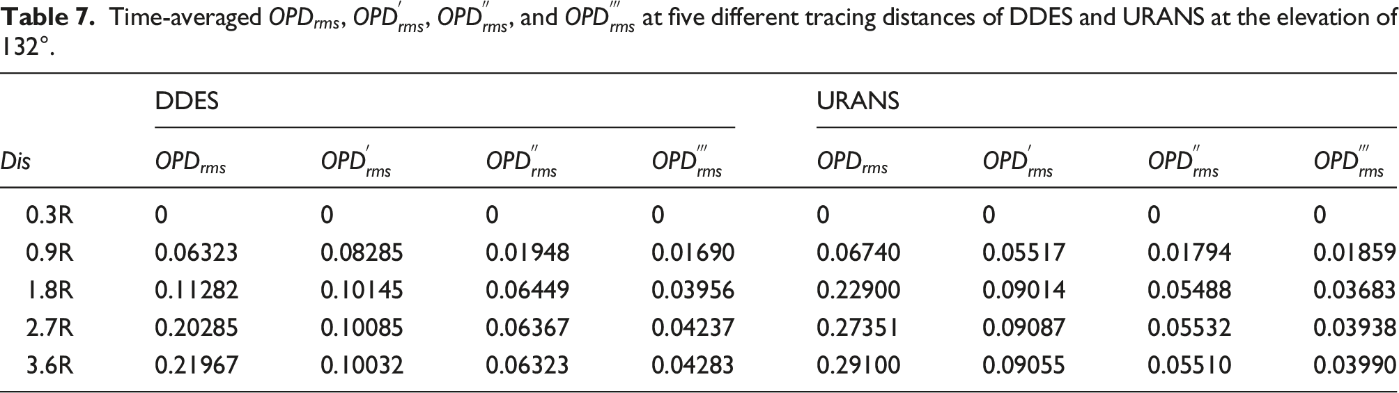
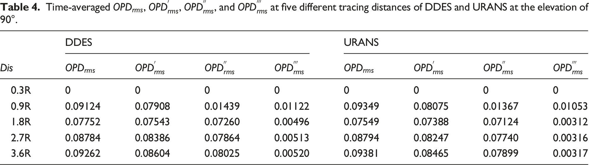
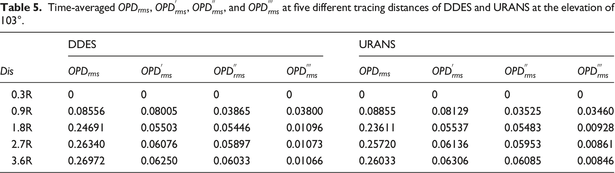
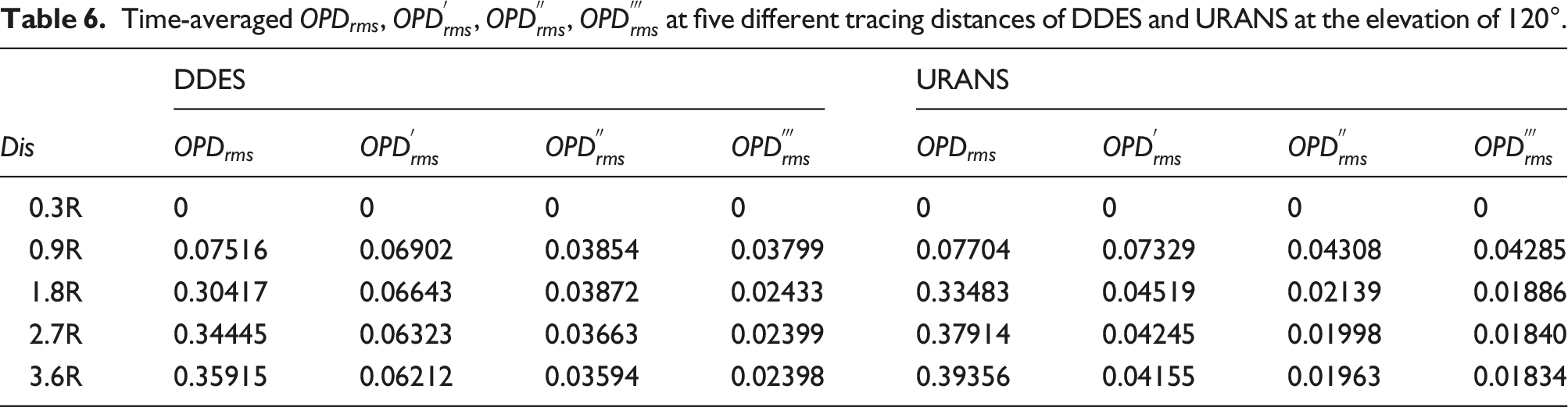
Time-averaged wavefront distortion, in terms of ${OPD}_{rms}$ , ${OPD}_{rms}^{\prime }$ , ${OPD}_{rms}^{″}$ , and ${OPD}_{rms}^{‴}$ , at different angles of elevation.

Particularly, at the distance of 0.9R, there is a maximal value of wavefront distortion, which is due to that the shape of conformal window influences laser beam transmission. When the central part of the laser beam has not reached the optical window, the rest part of the laser beam has passed through the optical window.

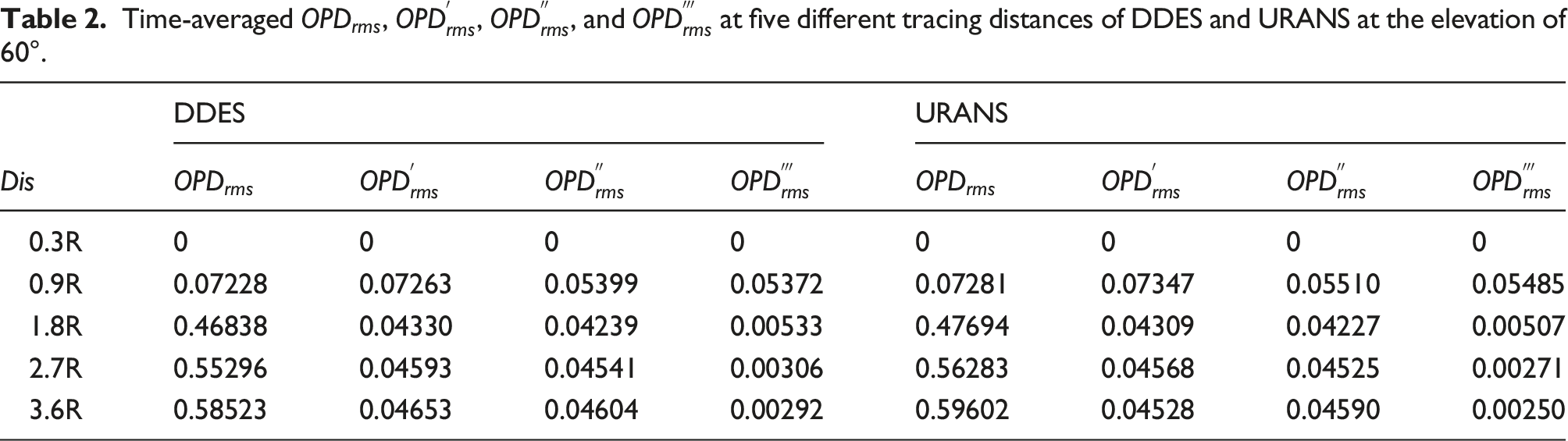
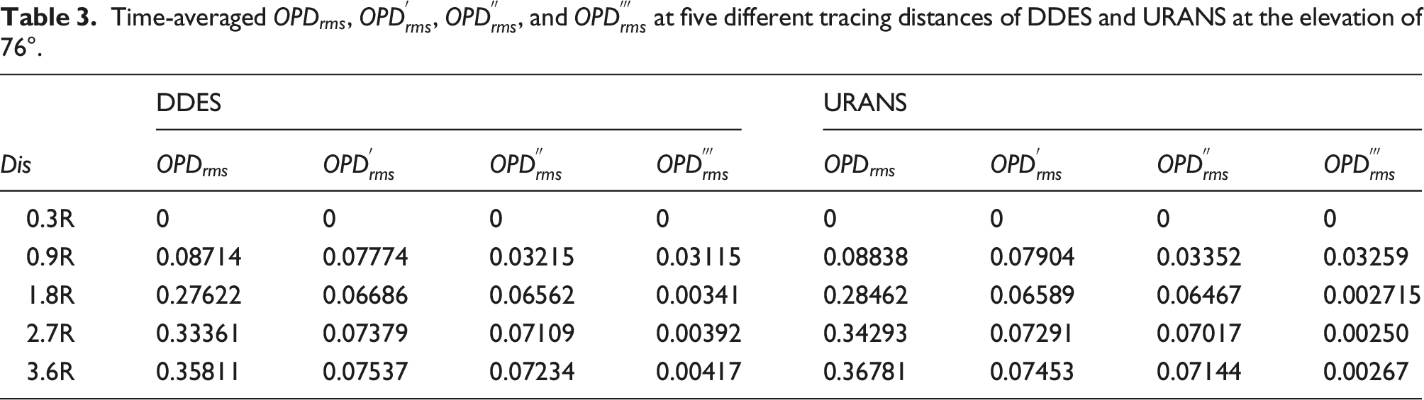
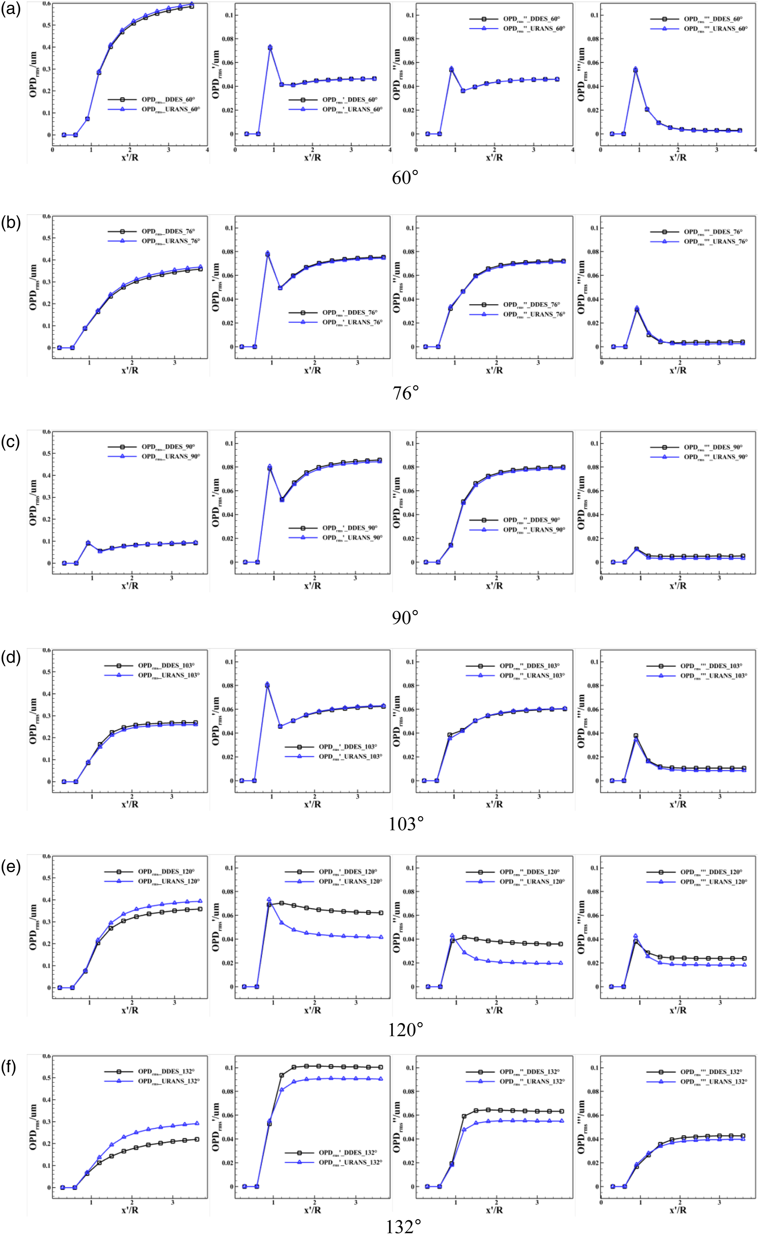
As plotted in Figure 30, the time-averaged OPD distribution of DDES and URANS are presented at six angles of elevation at different tracing distances. The time-averaged OPD is calculated over 100 instantaneous OPDs. The OPD distributions are generally similar of DDES and URANS, which is because the time-averaged density distributions of DDES and URANS are generally consistent with each other in laser transmission regions, as shown in Figure 26. Notably, the OPD distribution changes greatly in the region of 0.3–1.8R at all angles of elevation. In the region of 0.3–0.6R, the changes of OPD distribution are mainly caused by the shape of the optical window. In the region of 0.6–1.8R, the changes of OPD are caused by the inhomogeneous density distribution in the flow field.

Figure 30.

Time-averaged OPD distribution at five tracing distances of DDES and URANS at different angles of elevation.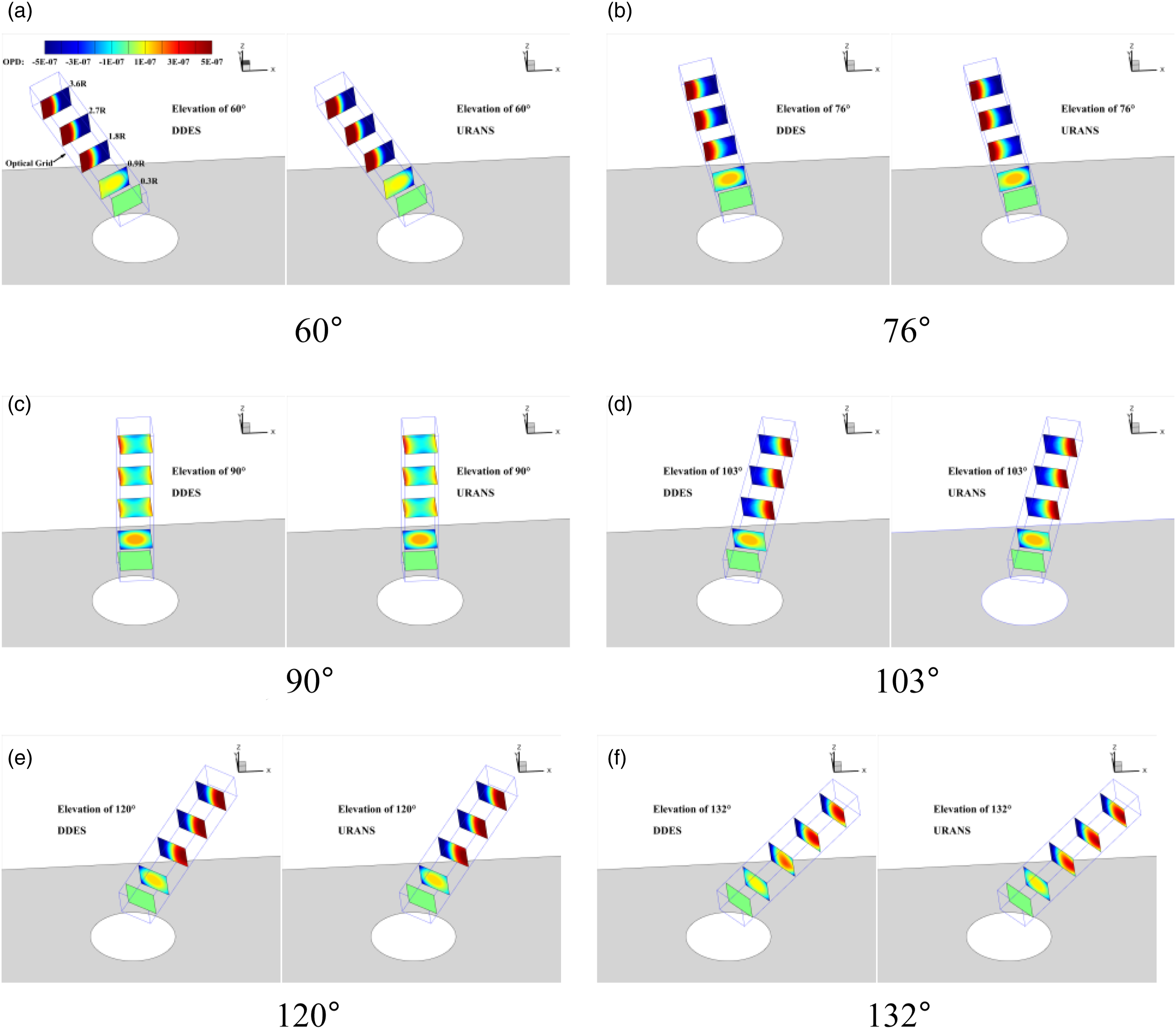

The temporal evolutions of the ${OPD}_{rms}$ , ${OPD}_{rms}^{\prime }$ , ${OPD}_{rms}^{″}$ , and ${OPD}_{rms}^{‴}$ at six angles are presented in Figure 31. At all angles of elevation, when the first six items are gradually removed, the fluctuation amplitudes gradually decrease, and the fluctuation frequencies gradually increase. At the four angles (60°, 76°, 90°, and 103°) located in attached flow regions, the frequencies of ${OPD}_{rms}$ , ${OPD}_{rms}^{\prime }$ , ${OPD}_{rms}^{″}$ , and ${OPD}_{rms}^{‴}$ are relatively high. However, when the laser beam is located in the separated regions, the frequencies of ${OPD}_{rms}$ , ${OPD}_{rms}^{\prime }$ , ${OPD}_{rms}^{″}$ , and ${OPD}_{rms}^{‴}$ are far lower than that in attached flow regions. In all plots, the fluctuations of frequency and amplitude of DDES are remarkably larger than that of URANS, which is due to that DDES can resolve more abundant turbulent fluctuations in the flow field. For ${OPD}_{rms}$ , ${OPD}_{rms}^{\prime }$ , ${OPD}_{rms}^{″}$ , and ${OPD}_{rms}^{‴}$ , the maximum amplitudes by DDES are about three to five times than that by UARNS. Notably, at six angles, ${OPD}_{rms}^{\prime }$ and ${OPD}_{rms}^{″}$ have the same frequencies, but the amplitudes are different. The difference between ${OPD}_{rms}^{\prime }$ and ${OPD}_{rms}^{″}$ is the defocus component, which is the stationary item in wavefront distortion, and the defocus component only affects the amplitudes rather than the frequencies. Therefore, the frequencies of ${OPD}_{rms}^{\prime }$ and ${OPD}_{rms}^{″}$ are similar.

Figure 31.

Temporal evolution of 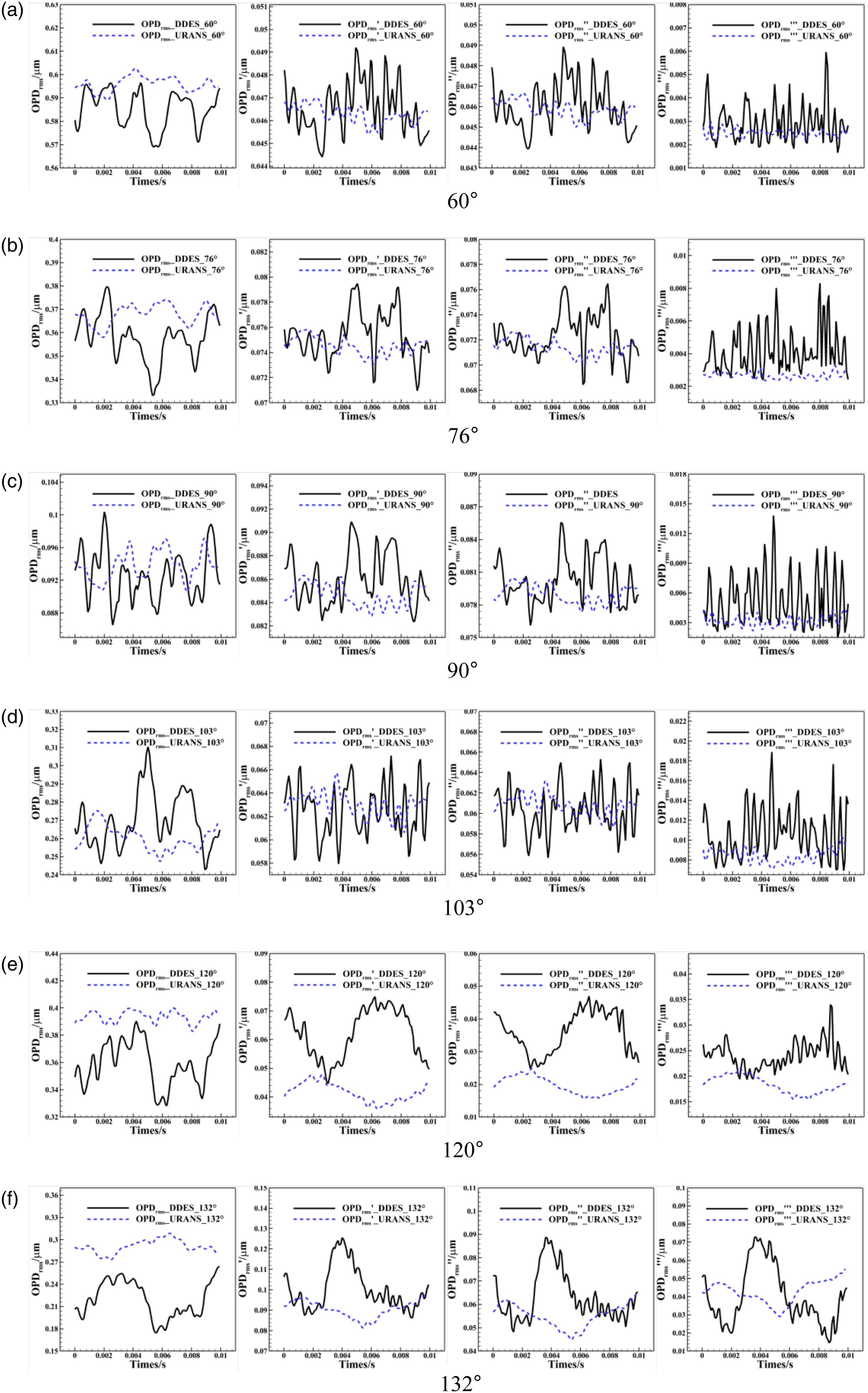${OPD}_{rms}$ , ${OPD}_{rms}^{\prime }$ , ${OPD}_{rms}^{″}$ , and ${OPD}_{rms}^{‴}$ at six different angles of elevation over the period of 0.01s.

Aero-optical effects influenced by Mach number and first-layer height (FLH)

In this section, the 3D turret with three Mach numbers (Ma = 0.2, 0.4, and 0.6) is investigated by using DDES, and the influence of two different first-layer heights (FLH) is also taken into consideration. Figure 32 shows the instantaneous stream velocity with four cases at Y = 0 slice. Flow separation, shear layers, and recirculation zones are reproduced in numerical simulations. At the case of Ma = 0.6, the wake shock wave appears, because the incoming Mach number is just close to the critical Mach number of 0.55. The recirculation zone of Ma = 0.6 is observably bigger than another cases. The separation point of Ma = 0.6 is closer to the turret zenith. Notably, as shown Figure 32(b) and Figure 32(c), at the two FLHs, the flow structures are almost similar.

Figure 32.

Instantaneous streamwise velocity at Y = 0 slice.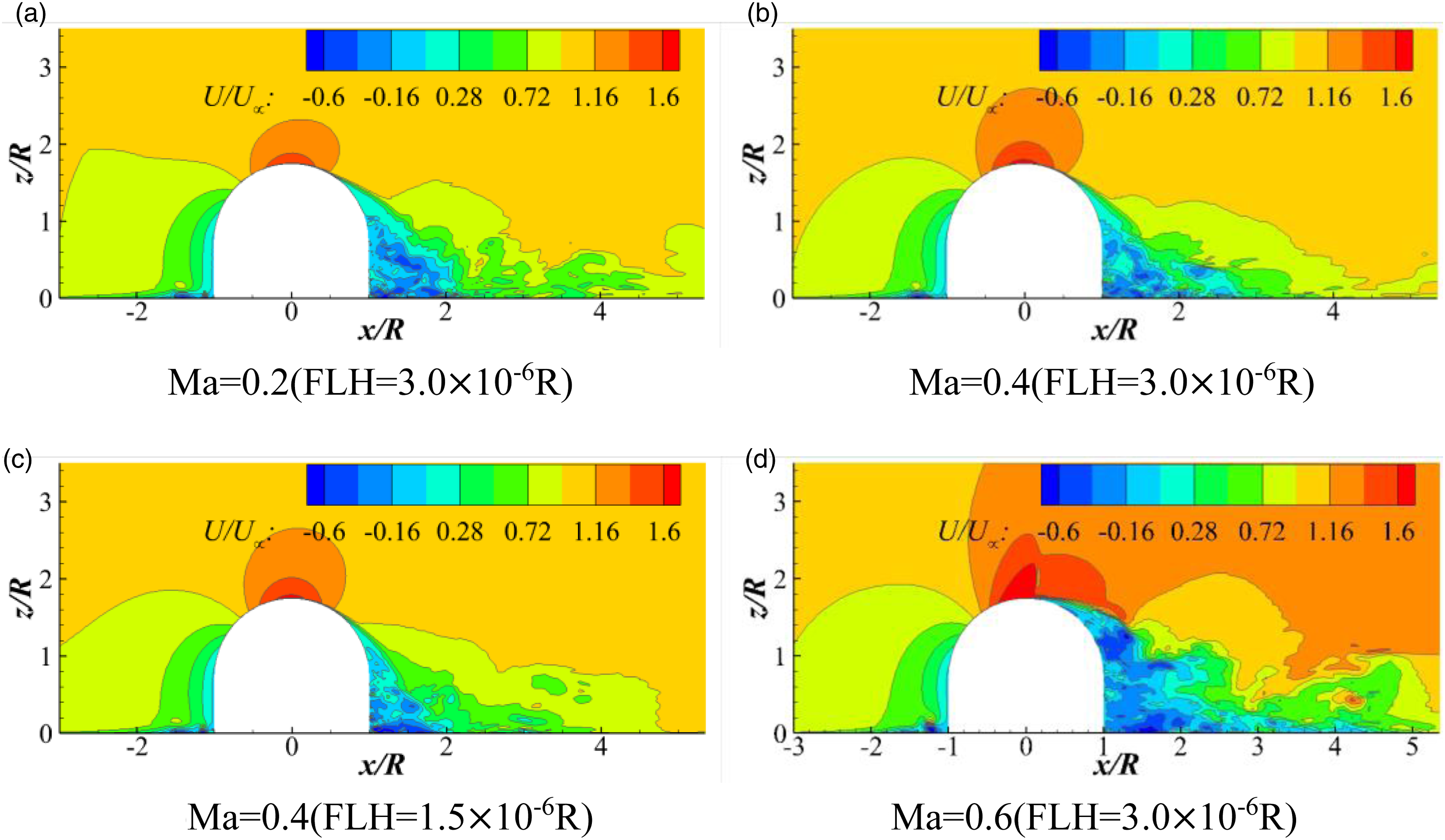

Figure 33 shows the time-averaged stream velocity with four cases at Y = 0 slice. The separation zone of Ma = 0.2 is slightly bigger than Ma = 0.4, except the case of Ma = 0.6. The flow structures of four cases are similar in the front of turret. Similarly, the recirculation zone of Ma = 0.2 are also slight bigger than the case of Ma = 0.4. The results indicate that with the increase of the Mach number, the separation point moves backwards and the recirculation zone is smaller. However, when the Mach number increases and the shock wave appears, the separation point is close to zenith. In addition, both time-averaged flow structures are only slightly different at the wake of the turret in cases with two FLHs.

Figure 33.

Mean streamwise velocity at Y = 0 slice.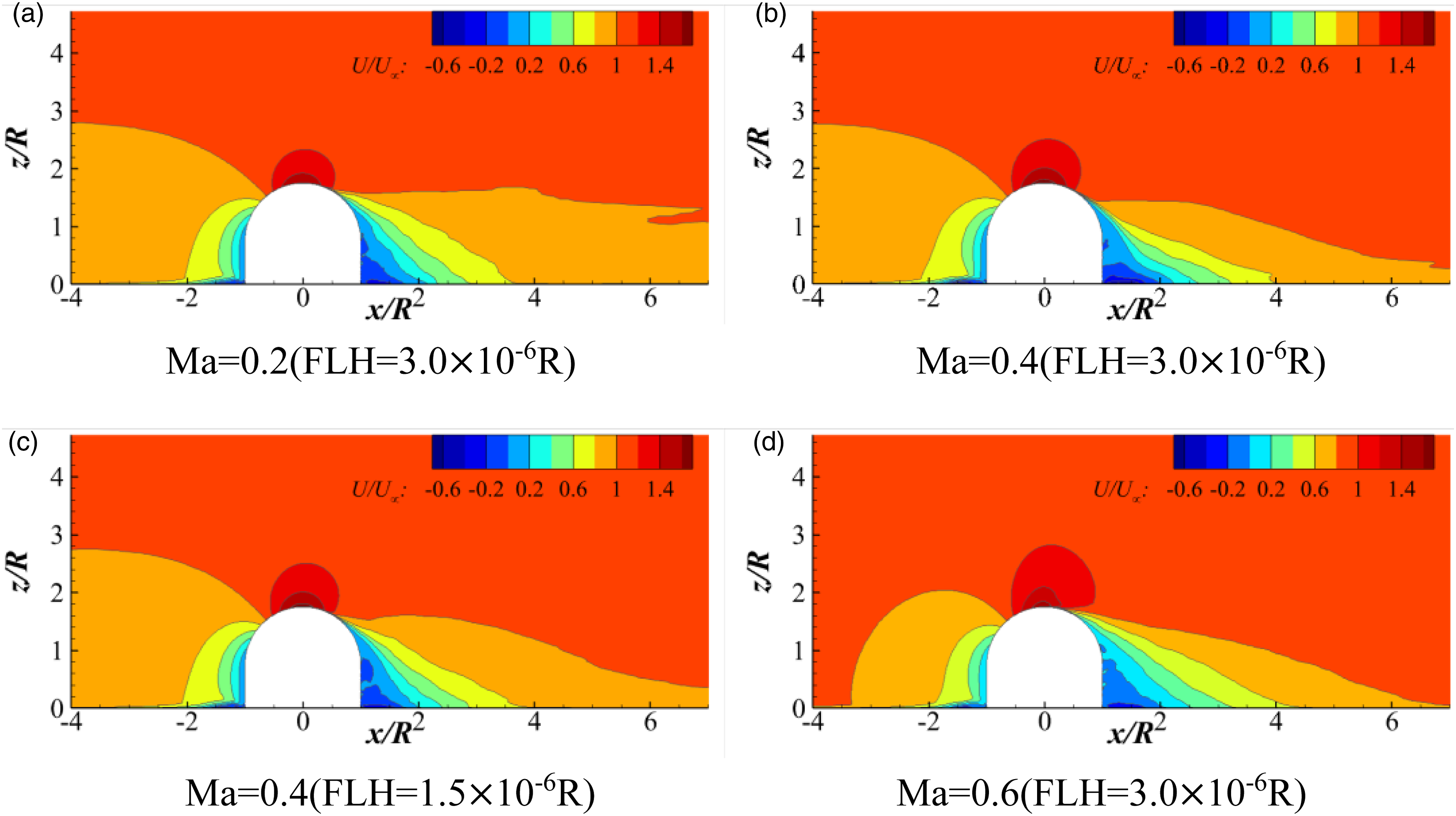

Figure 8 compares the velocity distribution in the boundary layer on turret at θ = 0°, 30°, 60°, 90°, 120°, and 150° for different Mach number and FLHs. It can be seen that the velocity profiles of two FLHs are totally similar, which indicates that the FLH = 3.0×10⁻⁶R is enough to capture the boundary layer flow. In the windward side, the velocity distributions of Ma = 0.2 and 0.4 are relatively same. In the backward side, the maximum velocity of Ma = 0.4 is relatively bigger than the case of Ma = 0.2, which is caused by the location separation point. The maximum velocity of Ma = 0.6 is smaller than the cases of Ma = 0.2 and 0.4 at six angles Figure 34.

Figure 34.

Velocity distributions in the boundary layer on the turret at θ = 0°, 30°, 60°, 90°, 120°, and 150°.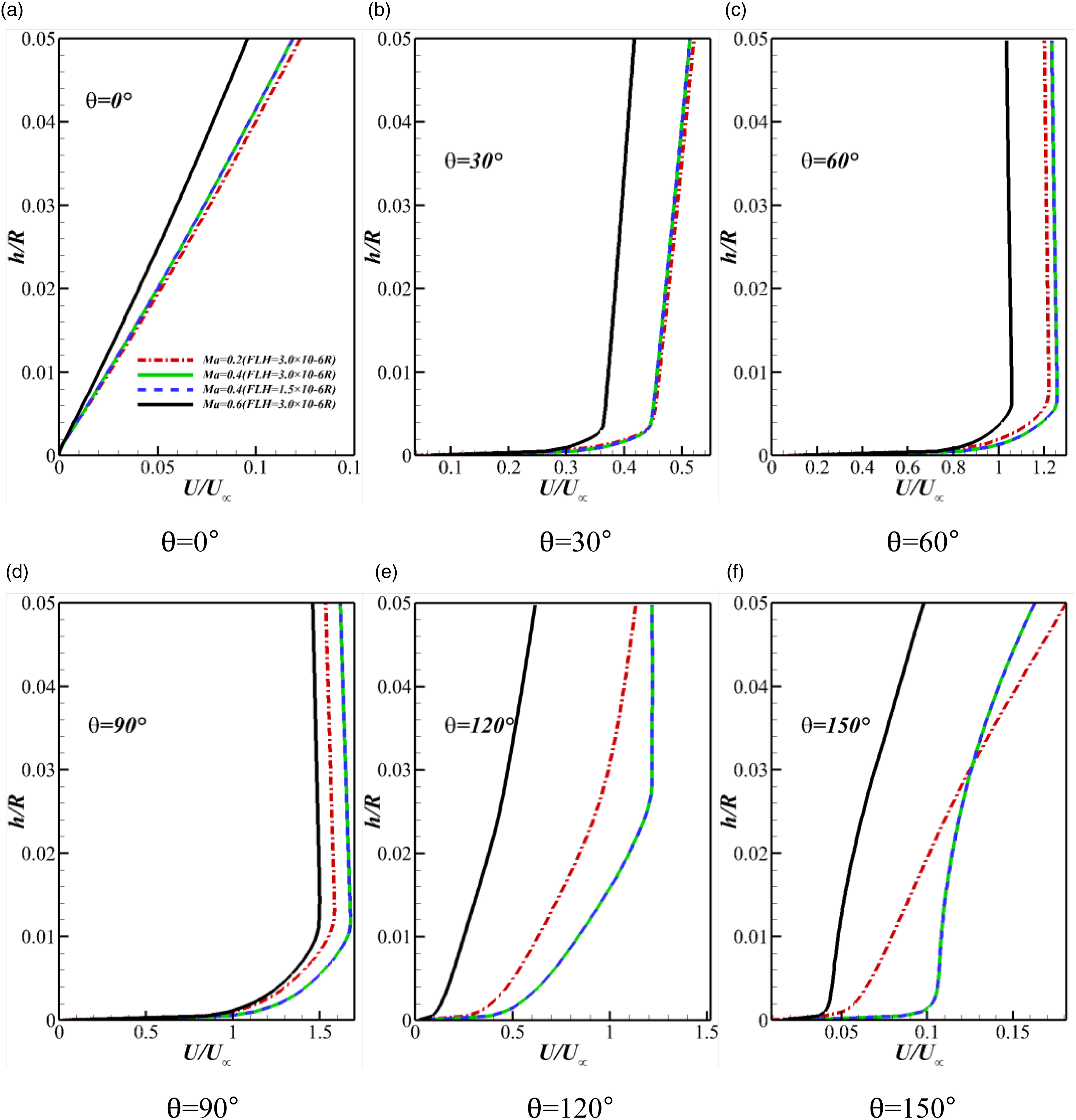

Figure 35 shows time-averaged wall pressure coefficient distributions along the turret centerline (Y = 0) obtained by DDES. Here, the pressure coefficient of two FLHs is also totally similar. The slight differences between the cases of Ma = 0.2 and Ma = 0.4 are in the region of θ = 60°–90° and θ = 150°–180°. At the case of Ma = 0.6, an obvious shock appears at θ = 90°–100°. Because the shock lead to the flow separation at the turret zenith, a bigger recirculation zone appears, which causes the smaller wall pressure coefficient in the backward of turret.

Figure 35.

Time-averaged pressure distribution along the turret centerline (Y = 0) for different Mach number and FLHs.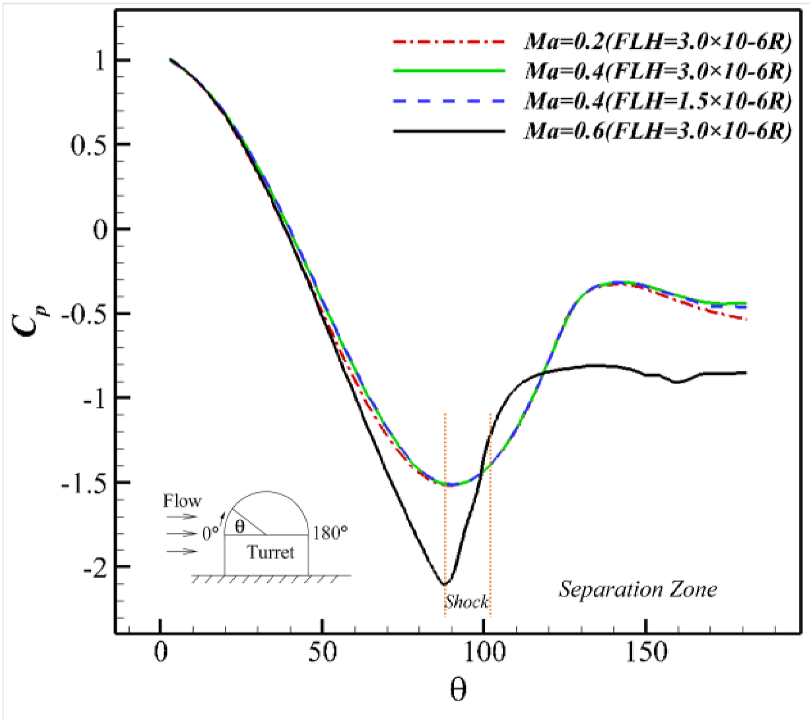

Figure 36 shows the wavefront distortions at the four cases. In the four sub-figures, the wavefront distortions at the cases of two FLHs are almost similar. In Figure 36(a)–(d), the obvious differences between the two FLHs are at θ = 120° and 132°, caused by the turbulent wake in the backward of the turret. The maximum relative errors of wavefront distortion at two FLHs are 2.7%, 9%, 2.7%, and 1%, respectively. And the tendency with θ is also similar. In Figure 36(a), the largest wavefronts are at θ = 60° at three Mach number, whose values are 0.114um, 0.585um, and 1.98um, respectively. The main reason is the large and steady density gradient in the windward side. In Figure 36(b)–(c), at the case of Ma = 0.6, after the steady component removed, the maximum wavefront is at θ = 90° or 103°, whose values are 0.804um, 0.665um, and 0.393um, which is caused by the shock wave. In general, the values of wavefront distortion increase sharply with the increase of Mach number. It can be concluded that compression has a big influence on the wavefront distortion, especially when the shock wave appears.

Figure 36.

Time-averaged wavefront distortions for different Mach number and FLHs, presented by OPDrms, OPDrms′, OPDrms″, and OPDrms‴.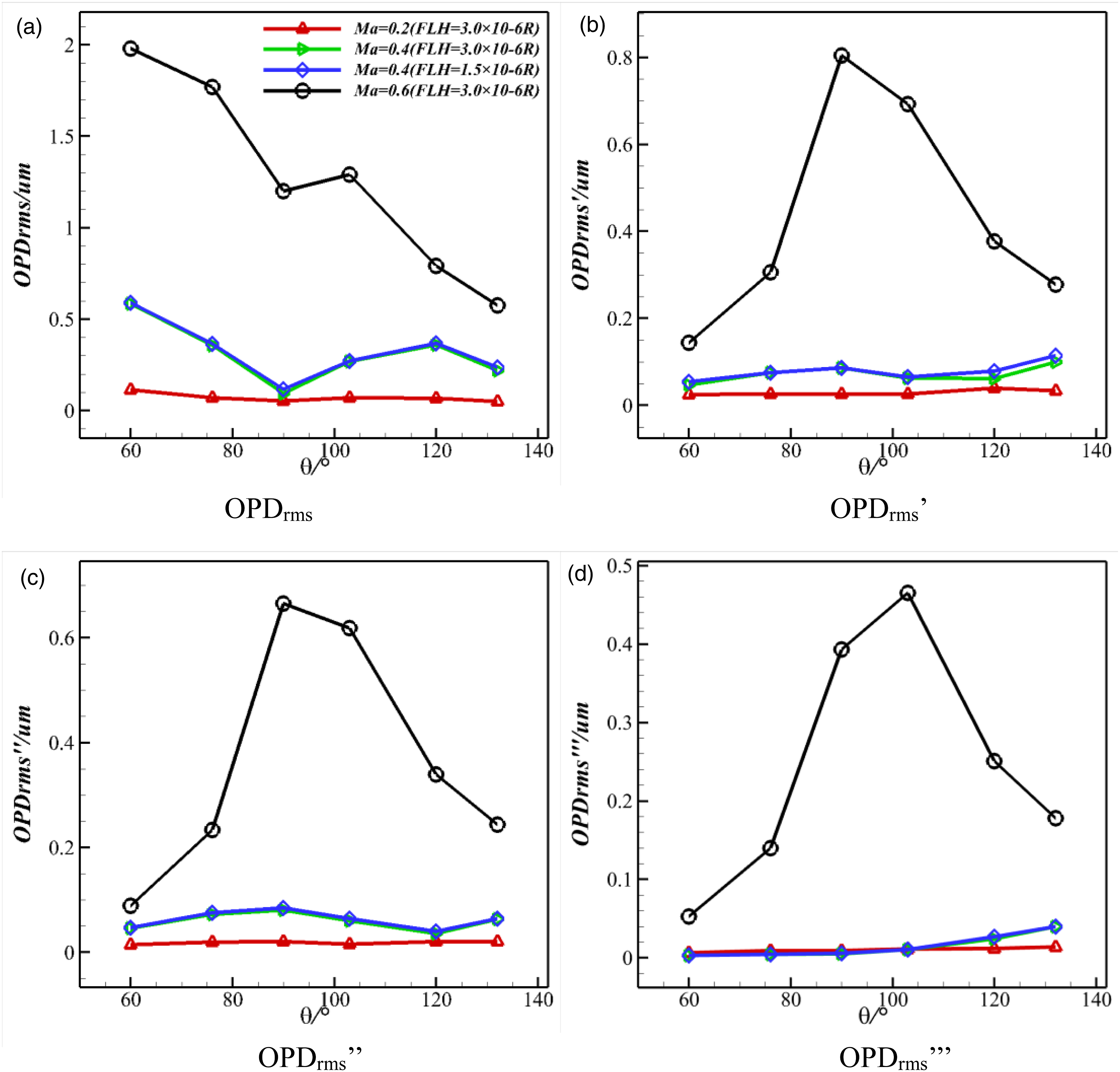

Conclusion

Based on the DDES-SST and URANS-SST, the unsteady flow around the turret is investigated on the platform ANSYSY CFX. The fine grid with 14 million cells and the coarse grid with 5 million cells are implemented to study the effect of the grid resolution. Instantaneous and time-averaged flow features are analyzed to assess the ability of DDES and URANS in resolving the flow field around the turret. Based on the density fields resolved by DDES and URANS, the fourth-order Runge–Kutta algorithm and the adaptive step size are used to trace the rays. Zernike polynomial is also applied to detailly analyze the wavefront distortion at six angles (60°, 76°, 90°, 103°, 120°, and 132°). The characteristics of spatial distribution and temporal frequency are also discussed in this work. In addition, aero-optical effects influenced by Mach number and first-layer height are briefly investigated. Several significant conclusions are obtained from this work.

(1) In the instantaneous flow features, DDES can capture abundant and high-frequency vortexes in the wake of the turret. URANS can only recognize the large and low-frequency vortexes because of the large numerical dissipation. The instantaneous density distributions of DDES at several sections are more disordered than that of URANS.

(2) In the time-averaged flow features, the pressure and density distributions at several sections of DDES and URANS are generally similar. Slight differences are present at the separated flow region. The pressure coefficient of DDES is also closer to the experimental data. Time-averaged surface flow features of DDES are the same with that of URANS in windward view, but different from that of URANS in leeward view. More typical structures on the surface of the turret can be captured by DDES. Time-averaged TKEs of DDES and URANS are totally different from each other. The time-averaged TKE peaks at values of about 596.2 and 1358 for DDES and URANS, respectively. The TKE of DDES is far smaller than that of URANS, because URANS have larger numerical dissipation.

(3) In spatial distribution of wavefront distortions, both results of DDES and URANS are slightly different from the experimental data at several angles. However, the wavefront distortions of DDES have good agreement with experimental data at angles of 120° and 132°, where the laser beam passes the separated flow regions. The time-averaged wavefront distortions of DDES and URANS are generally similar at the angles of 60°, 76°, 90°, and 130°, where the laser beam passes through the attached flow regions. In the region of the separated flow, the wavefront distortions of DDES are bigger than that of URANS, because more detailed information of density distribution can be captured by DDES. The maximal absolute differences of ${OPD}_{rms}^{″}$ and ${OPD}_{rms}^{‴}$ are at the angle of 120°, whose values are 0.0165μm and 0.0053μm, respectively.

(4) In temporal characteristics of wavefront distortions, at six angles, the frequencies and amplitudes of wavefront distortions of DDES are obviously higher than that of URANS, which is because more high-frequency structures in the flow filed can be resolved by DDES. The maximum amplitudes of wavefront distortion by DDES are about 3 to 5 times than that by URANS. The stationary item, defocus component, only affects the amplitudes of wavefront distortions rather than the frequencies.

(5) At the cases of two different FLHs at Ma = 0.4, the flow structures are totally similar, and the maximum error of wavefront is in OPDrms″ at θ = 132°, whose value is 9%. The tendency of wavefront distortion with θ is also similar. At the cases of three Mach number, the compression has a big influence on the wavefront distortion, especially when the shock wave appears.