Sage Journals: Discover world-class research

Abstract

The mechanism of flow separation in the impeller of a centrifugal pump with a low specific speed was explored by experimental, numerical, and theoretical methods. A novel delayed Reynolds-averaged Navier–Stokes/large eddy simulation hybrid algorithm combined with a rotation and curvature correction method was developed to calculate the inner flow field of the original pump for the large friction loss in the centrifugal impeller, high adverse pressure gradient, and large blade curvature. Boundary vorticity flux theory was introduced for internal flow diagnosis, and the relative velocity vector near the surface of the blade and the distribution of the dimensionless pressure coefficient was analyzed. The validity of the numerical method was verified, and the location of the backflow area and its flow features were determined. Finally, based on flow diagnosis, the geometric parameters influencing the flow state of the impeller were specifically adjusted to obtain a new design impeller. The results showed that the distribution of the boundary vorticity flux peak values, the skin friction streamline, and near-wall relative velocities improved significantly after the design change. In addition, the flow separation was delayed, the force applied on the blade was improved, the head under the part-load condition was improved, and the hydraulic efficiency was improved over the global flow ranges. It was demonstrated that the delayed Reynolds-averaged Navier–Stokes/large eddy simulation hybrid algorithm was capable to capture the separation flow in a centrifugal pump, and the boundary vorticity flux theory was suitable for the internal flow diagnosis of centrifugal pump.

Keywords

Pump improved delayed detached eddy simulation boundary vorticity flux hydraulic optimization flow separation

Introduction

Centrifugal pumps are used in aerospace, nuclear power, petrochemistry, and ocean engineering areas.^1,2 However, these pumps suffer from operational instability and technical limitations that affect their design and restrict their application. With strong rotation of the impeller flow passage, large curvature, viscosity, and a high adverse pressure gradient, unsteady flow structures such as flow separation, vortex, and secondary flow can occur. In addition, there are axial, radial, and peripheral vortices of different sizes. The flow separation is particularly intensive under the part-load conditions. This flow may exhibit intensive hydrodynamic characteristics, decreasing the operational efficiency of the centrifugal pump, shortening its service life, and potentially causing severe accidents. Thus, there is a significant need to study flow separation in the centrifugal pump and determine its mechanism.

In the past few decades, theoretical analyses, experiments, and numerical simulation methods have been used to study the problem of flow separation in a pump. Traditional methods evaluate flow stability based on such macroscopic information as velocity and pressure. However, these methods are incomplete and cannot be used to identify area of blade that required for improvement. To address this problem, many scholars have proposed new methods to study flow instability. Dou³ proposed a method to characterize flow instability based on an energy gradient and used this method to describe flow instability in various types of parallel flow geometric models and coaxial rotation cylinders. This method was successfully used by Zheng et al.⁴ to analyze the impact of the impeller passages on flow stability in the centrifugal pump. Li et al.⁵ investigated the variation of flow losses in a centrifugal pump based on the velocity distribution and entropy generation fields. Wang et al.⁶ proposed an energy loss model to optimize the design of a typical multistage centrifugal pump. Recent studies by Zhou et al.,⁷ and Zhang et al.⁸ introduced the theory of local vorticity dynamics diagnosis, taking advantage of its ability to significantly amplify unstable flow and examining the boundary vorticity flux (BVF) distribution on the impeller blade to investigate hydraulic performance. This approach was successfully used to provide a reference for vortex dynamics diagnosis to improve the hydraulic design of the centrifugal pump impeller.

Other studies have used particle image velocity (PIV) and pressure pulsation tests to study flow separation in a centrifugal pump. Yang et al.⁹ performed a hydraulic performance test on a centrifugal pump with a guide vane and detected two regions of H–Q curve instability under a low flow rate between 0.4Q_d and 0.7Q_d. And the flow separation structure in the flow passage between blades in the diffuser in the hump instability region was analyzed using a pressure pulsation test and high-speed flow visualization. Miorini et al.¹⁰ measured the complex flow field in the tip region of an axial water-jet pump using high-resolution PIV, revealed the evolution process of the tip leakage vortex, and found that the meandering of vortex filaments dominate passage flow. Keller et al.¹¹ measured the flow separation structure in a centrifugal pump with vaneless volute using two-dimensional PIV, analyzed the dynamic evolution of transient physical quantity in the pump with impeller rotation, used spectral analysis to characterize the energy at the blade-passing frequency, and elaborated the dynamic transmission process of the vortex within the impeller channel. Atif et al.¹² studied the flow structure of a mixed flow pump under off-design conditions using the PIV technique. The results showed that the instability of the performance curve was due to the rotating stall, and the pressure pulsation frequency spectrum exhibits two peaks, one correlating to the rotor–stator interaction frequency and its resonance frequency and the second correlating to the frequency of vortex shedding arising from separation of the boundary layer of the blade caused by the rotating stall. The flow separation in the pump was demonstrated to be an important source for the pressure pulsations and the radial loads fluctuations.¹³

Experimental investigation is difficult due to the inability to visualize the internal flow of a pump. As an alternative, with the improvements of computer hardware and the optimization of computational fluid dynamics (CFD) algorithms, numerical simulation has become an important tool to investigate flow.^14–16 In recent years, researchers have developed more effective methods to study pump flow. By reference to a dynamic hybrid model and a non-linear model, Yang and Wang¹⁷ proposed a hybrid non-linear subgrid-scale (SGS) model for large eddy simulation (LES) and conducted preliminary numerical research on the pump impeller of Pedersen.¹⁸ Compared with the PIV test, the hybrid non-linear SGS approach enables more accurate prediction of the low velocity zone in the flow passage and allows easier capture of the turbulent energy and the vortex structure in the turbulent flow field compared with the dynamic subgrid approach. Subsequently, Zhou et al.¹⁹ studied the detailed characteristics of the rotating stall in the impeller under a small flow using the above hybrid non-linear SGS model and proposed three evaluation parameters of a stall: blockage coefficient, stall cell size, and strength. Detached eddy simulation (DES) and delayed detached eddy simulation (DDES) methods developed by Spalart et al.²⁰ effectively combine the advantages of LES and unsteady Reynolds-averaged Navier–Stokes (URANS), and it can be used to process large separation flow with a large Reynolds number with limited computational resources. The DES-type or DDES-type methods have been widely applied to multiple types of flow simulation.^21–23

In this article, the improved delayed detached eddy simulation (IDDES) numerical method is used to study the internal separation flow. Internal flow in the impeller is diagnosed using boundary vorticity dynamics theory. And the position of flow separation generated within the centrifugal pump impeller is identified using BVF, the skin friction streamline, and the surface pressure distribution on a blade section at half span. The results are used to guide a new design for the impeller; as a result, the improvement on global hydraulic performance was achieved and pressure distribution on blade surface was stabilized.

Development of a novel IDDES hybrid method

IDDES hybrid methods

The IDDES²⁴ method is a DES-type method and is the latest version of a series of RANS/LES hybrid methods. In this work, the IDDES method proposed by Shur was used. This method combines characteristics of both DDES and WMLES (wall-modeled large eddy simulation) models and can solve the problem of “Log-Layer Mismatch” in the vicinity of the boundary layer and accelerate the conversion from RANS to LES in the separation zone. Compared with other DES models, IDDES further reduces the eddy viscosity coefficient of small subgrids in the logarithmic zone by redefining the LES scale near the wall surface. The conversion from the RANS zone to the LES zone is more accurate based on the definition of l_IDDES, the length scale of the wall surface model, thus avoiding insufficiency of the Reynolds stress modeling in the RANS zone and allowing the turbulent small-scale structure in the LES zone to be distinguished.

The IDDES model used in this article was created based on the k-ω shear-stress transport (SST) model with its transport equation as follows

\frac{\partial k}{\partial t} + u_{j} \frac{\partial k}{\partial x_{j}} = \frac{\partial}{\partial x_{j}} [(ν + σ_{k} ν_{t}) \frac{\partial k}{\partial x_{j}}] + P_{k} - \frac{k^{3 / 2}}{l_{IDDES}}

(1)

\frac{\partial ω}{\partial t} + u_{j} \frac{\partial ω}{\partial x_{j}} = \frac{\partial}{\partial x_{j}} [(ν + σ_{ω} ν_{t}) \frac{\partial ω}{\partial x_{j}}] + γ \frac{ω}{k} P_{k} \cdot f_{r} - β ω^{2} + 2 (1 - F_{1}) σ_{ω 2} \frac{1}{ω} \frac{\partial k}{\partial x_{j}} \frac{\partial ω}{\partial x_{j}}

(2)

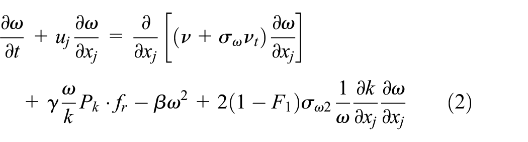
where the production term P_k reads as

P_{k} = υ_{t} S^{2} = 2 υ_{t} S_{ij} Ω_{ij}

(3)

where F₁ is the blending function, and the coefficients in the SST model are the following: σ_k₁ = 0.85, σ_ω₁ = 0.65, β₁ = 0.075, β^* = 0.09, κ = 0.41, $γ_{1} = β_{1} / β^{*} - σ_{ω 1} κ^{2} / \sqrt{β^{*}} \approx 0.46912$ , σ_k₂ = 1.0, σ_ω₂ = 0.856, β₂ = 0.0828, β^* = 0.09, κ = 0.41, and $γ_{2} = β_{2} / β^{*} - σ_{ω 2} κ^{2} / \sqrt{β^{*}} \approx 0.44035$ .

For the dissipation term in the k equation in the IDDES governing equation, l_IDDES is defined by

l_{IDDES} = {\tilde{f}}_{d} \cdot (1 + f_{e}) \cdot l_{RANS} + (1 - {\tilde{f}}_{d}) \cdot l_{LES}

(4)

The two working modes of the IDDES method are achieved by the conversion between the two types of length scales. The DDES length scale l_DDES and the length scale of the LES wall surface l_WMLES are defined as follows

l_{DDES} = {\tilde{f}}_{d} \cdot l_{RANS} + (1 - {\tilde{f}}_{d}) \cdot l_{LES}

(5)

l_{WMLES} = f_{B} \cdot (1 + f_{e}) \cdot l_{RANS} + (1 - f_{B}) \cdot l_{LES}

(6)

The definitions of l_RANS and l_LES differ from those in the DDES method.²⁰ The grid scale is modified as follows

Δ = min [max (C_{w} Δ_{max}, C_{w} d_{w}, Δ_{min}), Δ_{max}]

(7)

where the coefficients are as follows: C_w = 0.15; d_w = l_RANS = k^1/2/β^*ω; Δ_max = max (Δx, Δy, Δz); Δ_min = min (Δx, Δy, Δz); and Δx, Δy, and Δz are the grid length scale in the x, y, and z directions, respectively.

See Shur et al.²³ for the expressions of ~f_d, f_e, and f_B in the above functions.

Rotation and curvature correction

It is well known that k-ω SST turbulence model is one of linear eddy viscosity models (LEVMs), and the key weakness of existing LEVMs is that they cannot capture the effects of streamline curvature and system rotation, which significantly contribute to the turbulent flows of pumps. An efficient approach to resolve this issue was proposed by Spalart and Shur²⁴ and is described in the following.

The production term P_k of the k-ω SST model is multiplied by a coefficient, and it is defined by

f_{r} = max {min (f_{rotation}, 1.25), 0}

(8)

f_{rotation} = (1 + c_{r 1}) \frac{2 r^{*}}{1 + r^{*}} [1 - c_{r 3} \tan^{- 1} (c_{r 2} \tilde{r})] - c_{r 1}

(9)

The empirical constants c_r₁, c_r₂, and c_r₃ are set equal to 1.0, 2.0, and 1.0, respectively. The expressions of variables r^* and $\tilde{r}$ in equation (9) were described previously.²⁵

In this work, f_r is applied as a multiplier of the production term P_k in the original k-ω SST model as follows

P_{k} \to P_{k} \cdot f_{r}

(10)

The expressions of the mean stretching tensor S_ij and the intrinsic mean spin tensor Ω_ij are defined by

S_{ij} = \frac{1}{2} (\frac{\partial u_{i}}{\partial x_{j}} + \frac{\partial u_{j}}{\partial x_{i}})

(11)

Ω_{ij} = = \frac{1}{2} (\frac{\partial u_{i}}{\partial x_{j}} - \frac{\partial u_{j}}{\partial x_{i}}) + 2 ε_{jim} ω_{m}

(12)

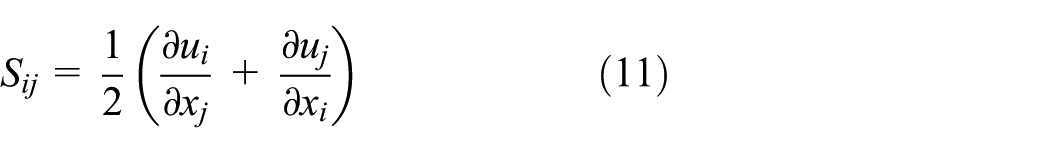
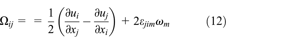
where ω_m is the vector form of angular velocity (m = 1, 2, and 3, representing the x, y, and z directions, respectively); ε_jim is the permutation symbol.

Numerical setup and description

Pump model

In this study, the above-described governing equations were solved by ANSYS-FLUENT 16.2. The low specific speed pump structure is shown in Figure 1, and the main geometric parameters of the pump are presented in Table 1.

Figure 1.

The impeller and volute.

Table 1.

Main pump parameters.

Parameter	Sign	Value	Unit
Flow rate at best efficiency point	Q _BEP	27	m³/h
Head at best efficiency point	H _BEP	11.6	m
Rotation speed of impeller	n	1450	r/min
Inlet diameter of impeller	D ₁	0.075	m
Outlet diameter of impeller	D ₂	0.198	m
Number of blades	z	6	–
Outlet blade angle	β ₂	42	°
Inlet blade angle	β ₁	33.6	°
Total blade wrap angle	γ	110	°
Outlet width of impeller	b ₂	0.009	m
Base circle diameter of volute	D ₃	0.22	m
Outlet diameter of volute	D ₄	0.05	m
Inlet width of volute	b ₃	0.033	m

BEP: best efficiency point.

Mesh generation

To increase the accuracy of numerical computation, a structured grid partition was used for the whole fluid domain. Different grid schematics were tested, as shown in Figure 2. A local refined mesh was applied near the wall, and the y+ value near the boundary wall was lower than 50. A grid independence analysis was conducted before computation. As can be seen in Figure 2, in Schemes 3–5 (more than ∼1.57 million grids), the pump head fluctuates little with increased grids. Therefore, Scheme 4 was adopted.

Figure 2.

Grid independency study data.

The grids of impeller and volute are shown in Figure 3.

Figure 3.

Grids of pump model.

Solution parameters

The time-dependent governing equations were discretized in both space and time domains. A high-resolution scheme was adopted for the advection term, and a second-order backward Euler algorithm was used for the transient term. The equations used the finite volume method for dispersion in space and used the second-order implicit scheme for dispersion in the time domain. A time step of 0.001149 s was used, equal to 1/360 of the rotation period. For spatial differences in physical quantity, the diffusion term included the second-order central difference. The decoupling of the velocity pressure used the semi-implicit method for pressure-linked equations-consistent (SIMPLEC) algorithm. To balance computational resources and accuracy, the residuals were 10⁻⁵ for 20 iterations in each time step in this study.

To rapidly achieve computational stability, the improved SST steady-state model was used to solve a steady flow field result and the steady-state case result as the initial flow field for the unsteady simulation. The IDDES model was used with the above initial values. Sufficient computational time was used to guarantee accurate statistics (average velocity and average pressure) in the flow field after stabilization of the flow. The computation proceeded for 20 revolutions of the impeller. Given that the goal was to understand the mechanism of flow separation, the following flow conditions were selected: 1.2Q_BEP, 1.0Q_BEP, 0.8Q_BEP, 0.6Q_BEP, 0.4Q_BEP, and 0.2Q_BEP.

Results and discussion

Flow field visualization experiments

The hydraulic performance and PIV inner flow experiments were performed in the laboratory of the Research Center of Fluid Machinery Engineering and Technology of Jiangsu University, as shown in Figure 4. The PIV test errors, pressure sensor calibration, motor speed, shaft power, and flow measurement uncertainty analyses for this pump are discussed in detail in literature.^26,27

Figure 4.

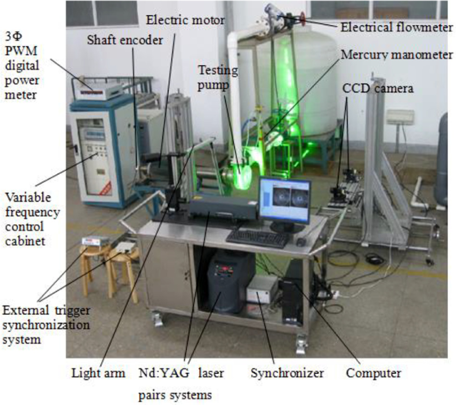
Test system.

The test region of the impeller is illustrated in Figure 5, and the six different flow passages are named as no. 1 to 6. In the test, three sections of the impeller flow passage were selected in the midsection and sections near the shroud and hub. To determine the photographed section of the shroud and hub, the laser sheet was adjusted to fit to the surface of the shroud and hub. The laser sheet is 1–2 mm. To avoid the interference from shroud and hub, the distance between the imaged section and the shroud and hub was 0.5–1 mm. The imaged section is shown in Figure 6. Sections 1, 2, and 3 in Figure 6 represent the cross section near the shroud, middle section, and the cross section near the hub, respectively. To explore the working conditions that lead to flow separation, the flow rate was decreased from 1.2Q_BEP to 0.1Q_BEP. The changes in the flow structure in the impeller were observed as flow was decreased. For simplicity, only the flow field in section 2 was analyzed.

Figure 5.

Schematic diagram of testing region.

Figure 6.

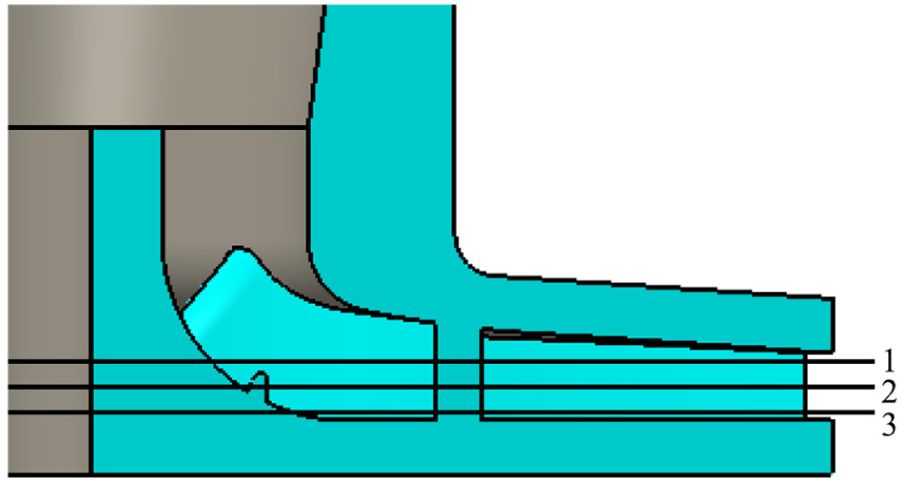
Schematic diagram of the test section.

Figure 7 presents the distribution of relative velocities from high flow to low flow within the section near the middle. The following conclusions can be drawn from the results:

Under the large flow rate, the low velocity zones are formed near the pressure surface (PS) and areas of high velocity were near the suction surface (SS). Thus, the SS is relatively more stable than the PS. With decreased flow rate and under the action of impeller rotation, the low momentum fluids near the PS increased gradually, causing the high momentum fluids near the SS to move toward the exit.

The high-speed revolution of the impeller would cause flow separation to occur near the PS. A separation vortex starts to develop on the PS of Passage 1 at 0.6Q_BEP. With decreased flow, the area of the separation vortex increases gradually, and the core area of the vortex separates from the PS. A large separation vortex forms move toward the middle and concentrate at the impeller outlet.

In Passage 1, the number of separation vortices and the vortex intensity decrease with the decrease in flow rate. At 0.4Q_BEP, the separation vortex starts to evolve from a single vortex to double vortices. The action range of the vortex cluster increases with the flow decrease, and separation vortex occurs in multiple flow passages. At 0.2Q_BEP, the multiple-vortex structures converge into a large vortex cluster, which blocks the flow passage at the impeller outlet.

The separation vortices first appear in several flow passages close to the tongue, particularly in Passage 1. With the decrease in flow, the separation vortices expand into other flow passages. The streamline in Passage 6 starts to show disorder at 0.6Q_BEP. Separation vortices occur on the PS at 0.4Q_BEP. The single vortex evolves into multiple vortex systems and expands toward the outlet with decreased flow. Under the whole flow range, no obvious flow separation occurs in Passage 5 and the streamlines in this passage are smoother than those in other flow passages, which may reflect effects of the relative position of the flow passage.

Figure 7.

Relative velocity distribution in section 2 under different flow conditions (unit: m/s): (1) 1.2Q_BEP, (2) 1.0Q_BEP, (3) 0.8Q_BEP, (4) 0.6Q_BEP, (5) 0.4Q_BEP, and (6) 0.2Q_BEP.

Behind the hub, Passages 2 and 3 are in the dark region because the impeller hub blocks the laser, so the laser intensity in this area is weak. The uneven distribution of laser in this area leads to more red spots and blue spots in Passages 2 and 3 than in other passages. Thus, there are significant errors in the velocity field in this area. Also, as can be seen in Figure 7, the streamlines in Passages 2 and 3 are less smooth than those in other passages under various working conditions, so these are not included in the analysis of velocity fields.

Evaluations of the numerical framework

Figure 8 compares the pump head versus flow rate (H–Q) curves. The rotating speed of the pump is 1450r/min. As shown in Figure 8, the parameters of the pump at the best efficiency point (BEP) are as follows: flow rate Q_BEP = 27.72 m³/h and head H_BEP = 11.58 m. The specific speed was n_s = 74 at the BEP (n_s = 3.65nQ^1/2/H^3/4).

Figure 8.

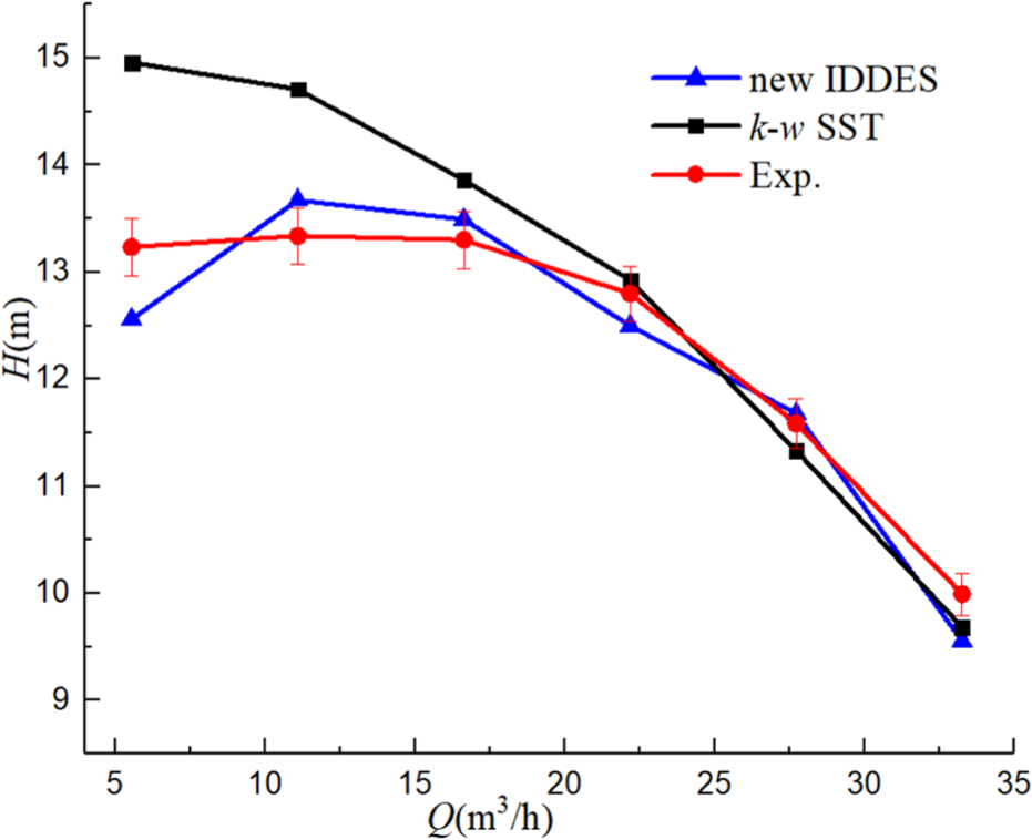
Comparison of hydraulic performance between experimental and numerical results.

The new IDDES model computation results were more consistent with the experimental data than the original one, especially when the flow rate was lower than 0.6Q_BEP (17 m³/h). According to the H–Q curves, the head relative discrepancies by new IDDES model were about 5% both at 0.2Q_BEP (6 m³/h) and 1.2Q_BEP (33 m³/h), but the head relative discrepancies under other flow conditions were all less than 2.5%. There were some differences between the actual experimental model and the ideal model of numerical calculations that were attributable to the manufacturing process (e.g. stamping and welding). The observed deviations also may be attributable to uncertainties in the instruments, apparatus, and pipeline system during the test. Leakage from the wear ring was neglected in the simulation. Overall, the results show that the new numerical method is credible.

It can be seen from Figure 7 that the separation vortex started at 0.6Q_BEP. Therefore, in order to further compare with the PIV test, the development of separation flow in the section 2 under 0.6Q_BEP was investigated in Figure 9. As the impeller rotating at different angles, it indicated that the new model was more accurate than the original model in terms of the range of low speed zone near the PS, the range of high speed zone near the SS at the impeller inlet, the jet-wake flow at the impeller exit and the structure vortex in passage 1.

Figure 9.

Comparison of the numerical predicted and experimental separation flow evolutions under 0.6Q_BEP. (1) Exp. result at 0.6Q_BEP: (a) 0T, (b) 1/3T, and (c) 2/3T. (2) Cal. result by original model at 0.6Q_BEP: (a) 0T, (b) 1/3T, and (c) 2/3T. (3) Cal. result by new IDDES model at 0.6Q_BEP: (a) 0T, (b) 1/3T, and (c) 2/3T.

BVF internal flow diagnosis

BVF is the core concept of boundary vorticity dynamics, originating from the boundary vorticity model proposed by Lighthill²⁸ in 1963. A source of vorticity at a solid wall is not only the tangential pressure gradient but also acceleration of the wall, curvature, and skin friction. For a constant rotational speed, the acceleration term is zero. For high Reynolds number, the contribution of skin friction is negligible and the effect of curvature is small (except at sharp edges and corners). This is why, for a high Reynolds number and away from sharp corners, the BVF reduces to equation (13)

σ_{P} = - \frac{1}{ρ} \overset{⌢}{n} \times \nabla p

(13)

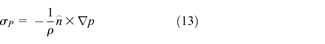
where $\overset{⌢}{n}$ is the unit normal vector pointing out of the fluid and ρ is the density of fluid.

In an incompressible fluid field with conservative body force, BVF is the root cause of the occurrence and diffusion of vorticity and can induce a series of flow separation phenomena such as boundary layer separation, secondary flow, or large-scale separation. Wu and colleagues^29,30 established the theory of boundary vorticity dynamics. The torque applied on the blade can be obtained by integration

M_{y} = - \frac{1}{2} \int_{S_{b}} ρ r^{2} σ_{py} dS + \frac{1}{2} \oint_{\partial S_{b}} p r^{2} dy

(14)

where r is the radius of impeller, S_b is the blade surface, ∂S_b is the boundary of the blade surface, σ_py is the axial component of the boundary vorticity flow σ_p caused by the pressure gradient of the blade surface, and p is the pressure. As can be seen in formula (14), controlling the distribution of BVF on the blade surface can inhibit flow separation and improve the force applied on the blade, thus optimizing impeller design.

The skin friction vector is an important basis to evaluate flow separation. Its expression is

τ = - μ ω \times n

(15)

where μ is dynamic viscosity, ω is the vorticity, and n represents the unit normal vector outward from fluid. According to the judgment criterion for flow separation, the skin friction streamline converged in the flow separation zone.

Based on the above analysis of PIV results, the flow separation in the impeller flow passage starts at the PS of blade 1 close to the tongue and increases in Passage 1. BVF contour distribution on the PS and SS of blade 1 was computed with the improved IDDES method, Surface 1 is illustrated in Figure 10, and is offset by 0.5 mm from the blade surface. The simulated data by the improved IDDES method for the skin friction streamline and the velocity distribution on Surface 1 are presented in Figure 11.

Figure 10.

Schematic of Surface 1 and positions of monitoring points (TE: tail edge; LE: leading edge).

Figure 11.

Distribution of σ_py and skin friction streamline on blade 1 and velocity vector on Surface 1: (1) BVF distribution on the PS surface of blade 1 under different flow conditions: (a) 1.0Q_BEP, (b) 0.8Q_BEP, (c) 0.6Q_BEP, (d) 0.4Q_BEP, and (e) 0.2Q_BEP. (2) BVF distribution on the SS surface of blade 1 under different flow conditions: (a) 1.0Q_BEP, (b) 0.8Q_BEP, (c) 0.6Q_BEP, (d) 0.4Q_BEP, and (e) 0.2Q_BEP.

According to formula (14), the σ_py peak value, either positive or negative, indicates excessively large pressure gradient in this area. A dramatic stress change should be avoided. As can be seen in Figure 11, a large pressure gradient and a positive peak value of σ_py occur at the leading edge due to the severe impact from the flow. A negative peak area occurs at the tail edge, indicating the large pressure gradient in this area is due to rotor–stator interaction. However, in the middle area of the impeller flow passage, when the flow rate decreased to 0.6Q_BEP, there was a strip of σ_py positive peak area on the PS. When the flow further decreased, the σ_py positive peak area expanded toward the tail edge, indicating a dramatically increased vorticity generation rate. This spatial accumulative effect finally would lead to large-scale separation. Thus, a high and steep σ_py positive peak is a precursor of large-scale separation. Based on the skin friction streamline and the distribution of relative velocity vectors on Surface 1, under the flow condition of 0.6Q_BEP, flow separation occurred in the σ_py positive peak area. This is the area where the skin friction streamline converged to a point. Back flow areas completely opposite to the main flow areas started to occur in this area. With a further decrease in flow, the flow separation area moved toward the tailing edge. The area of the back flow area also expanded, as indicated by the distribution of velocity vectors. Compared with the PS, the SS had a more even distribution of σ_py. Based on the distribution of the skin friction streamline on the SS and the relative velocity vectors on Surface 1, when the flow decreased to 0.2Q_BEP, back flow occurred and this area almost covered the whole flow passage from the inlet to the outlet. Overall, the simulated data are consistent with the PIV results.

The dimensionless pressure coefficient distribution (c_p = (p − p_inlet)/(0.5ρu₂²)) on the intersection line between the middle section of the flow passage and the blade surface was quantitatively analyzed. As can be seen in Figure 12, the value of C_p of the PS is larger than that of the SS under large flow. When the flow decreases to 0.6Q_BEP, the pressure of the SS is larger than that of the PS when the blade surface pressure along the flow direction length is 0.7. This corresponds to the positive peak area of σ_py and is consistent with the start of flow separation at the initial flow condition of 0.6Q_BEP. As flow decreases, the area with a SS larger than the PS expands to the outlet and almost occupies the whole flow passage under 0.2Q_BEP, suggesting that negative work applied on the fluid here.

Figure 12.

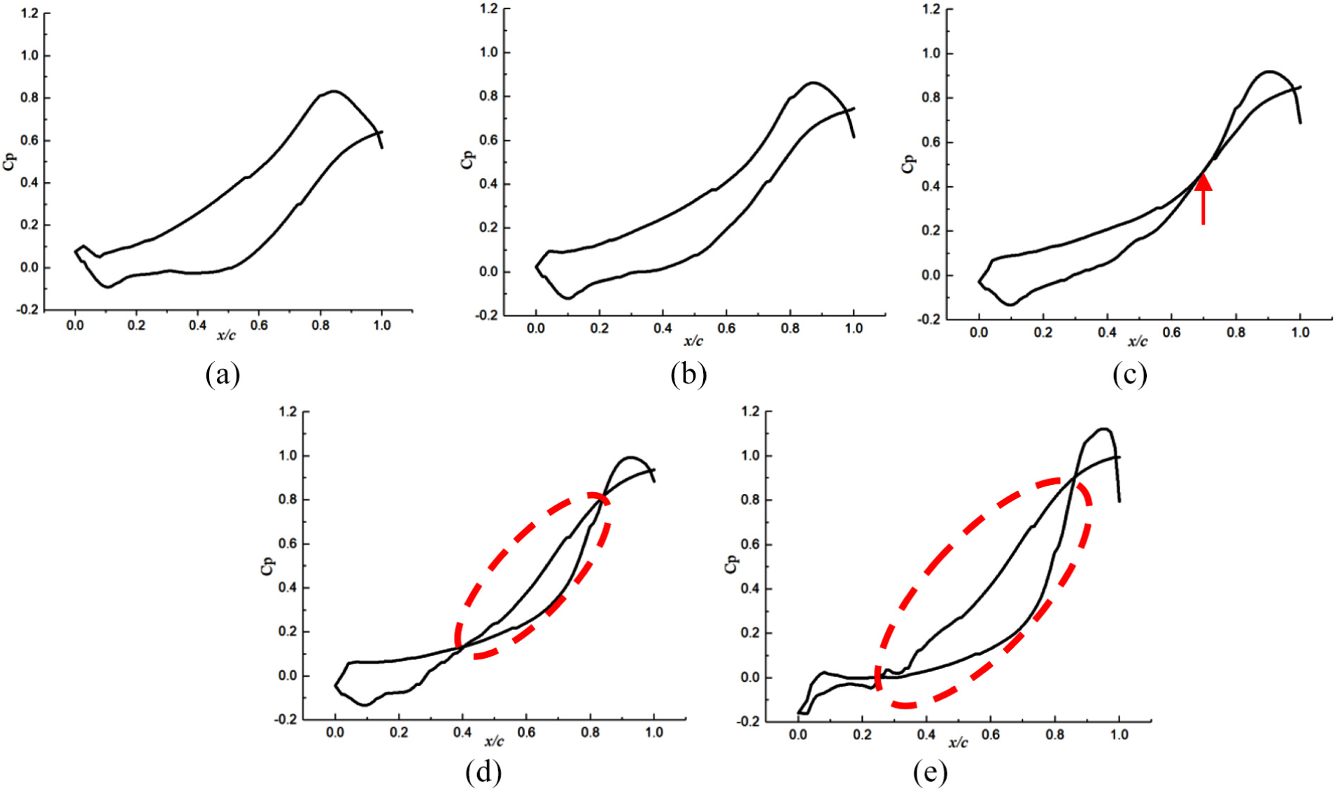
Distribution of pressure coefficients on the middle lines of the blade: (a) 1.0Q_BEP, (b) 0.8Q_BEP, (c) 0.6Q_BEP, (d) 0.4Q_BEP, and (e) 0.2Q_BEP.

The BVF diagnosis and distribution of dimensionless pressure coefficients can reflect the conditions of pressurization and help identify design defects. There was a large area from the middle part of the PS to the trailing edge with a high-pressure gradient, suggesting unreasonable pressurization. Thus, the optimization design should focus on the PS.

Blade redesign and analysis

Redesign for blade

The problems of the original impeller blade 1 present from the middle of the PS to the tailing edge suggest that the area has a large curvature, thus making the flow angle inconsistent with the blade angle and increasing the risk of flow separation close to the blade surface. Thus, the blade angles over the entire length of the blade are reduced, by the way, the wrap angle of blade and outlet width of the impeller are increased. This normally leads to a steeper H–Q curve and helps to make the blade load more even. Thus, the difference between the flow angle and the blade angle is decreased to eliminate flow separation in the flow passage. And further, this prevents the hump at part-load conditions (since stall will inevitably happen at low flow rate). The major geometric parameters of the impeller following optimization are shown in Table 2. Figure 13 presents the comparison between the original blade and the optimized blade.

Table 2.

Main pump parameters.

Parameter	Sign	Value	Unit
Inlet diameter of impeller	D ₁	0.075	m
Outlet diameter of impeller	D ₂	0.198	m
Number of blades	z	6	–
Outlet blade angle	β ₂	26.5	°
Inlet blade angle	β ₁	30	°
Total blade wrap angle	γ	120	°
Outlet width of impeller	b ₂	0.01	m

Figure 13.

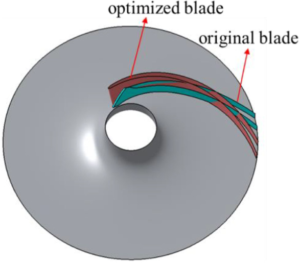
Comparison between the original blade and optimized blade.

Analysis of results

The optimized impeller was subject to three-dimensional reconstruction, mesh partitioning, and numerical computation. The boundary conditions and computational methods were the same as those used for the original impeller. After computation, a contour of σ_py distribution on the surface of the optimized impeller was obtained according to formulas (15)–(17), as shown in Figure 14. As can be seen in the diagram, the distribution of σ_py on the PS of the optimized blade is significantly more uniform; the σ_py positive peak at the leading edge also decreases substantially. A strip-shaped σ_py positive peak area in the middle of the flow passage still exists, but the peak occurs at 0.4Q_BEP instead of 0.6Q_BEP. According to the distribution of the skin friction streamline and the surface relative velocity vectors, the skin friction streamline starts to converge at 0.4Q_BEP. An obvious back flow area occurs also at 0.4Q_BEP. This indicates that the optimized impeller inhibits the back flow area in the flow passage, and the hydraulic loss is reduced and the efficiency is improved for the optimized impeller.

Figure 14.

Distribution of σ_py and skin friction streamline on the optimized blade 1 and velocity vector on the Surface 1. (1) BVF distribution on the PS surface of blade 1 under different flow conditions: (a) 1.0Q_BEP, (b) 0.8Q_BEP, (c) 0.6Q_BEP, (d) 0.4Q_BEP, and (e) 0.2Q_BEP. (2) BVF distribution on the SS surface of blade 1 under different flow conditions: (a) 1.0Q_BEP, (b) 0.8Q_BEP, (c) 0.6Q_BEP, (d) 0.4Q_BEP, and (e) 0.2Q_BEP.

Comparison of Figures 11 and 14 reveals that the significant difference in flow field distribution between the original blade surface and the optimized blade surface starts to occur at 0.6Q_BEP. Figure 15 presents the distribution of skin friction coefficients on the middle lines on blade 1 before and after optimization. As can be seen in the diagram, the original blade PS has a large area (x/c = 0.08–0.7) with a small skin friction coefficient. The skin friction coefficient approximates 0 at x/c = 0.57, indicating the presence of a separation flow here, which basically corresponds to the position where the back flow occurs in Figure 11. The skin friction coefficient of the SS of the original impeller fluctuates considerably. The skin friction coefficient decreases dramatically near the leading edge, in the middle part of the blade, and at the tailing edge, likely due to the vortex structure on the PS. The optimized skin friction coefficient was decreased substantially at the leading edge. In the middle part, there is an area (x/c = 0.2–0.65) with a small skin friction coefficient that is larger than the skin friction coefficient in the same position for the original impeller. In addition, the optimized SS skin friction coefficient fluctuates gently, indicating small energy dissipation, conducive to the improvement of the pump efficiency.

Figure 15.

Comparison of the skin friction coefficient on the middle profile between the original blade and optimized blade.

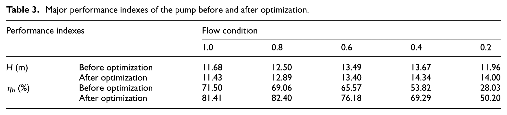
Table 3 compares the major performance indexes of the original pump and optimized pump. As can be seen in the table, the head of the optimized pump is basically consistent with that of the original centrifugal pump for flow ranging from 0.6Q_BEP to 1.0Q_BEP. The head is increased significantly at 0.2Q_BEP and 0.4Q_BEP, and the hump of the H–Q curve of the original centrifugal pump is eliminated. The hydraulic efficiency of the optimized pump improved significantly, indicating that the optimized impeller has less loss and higher efficiency.

Table 3.

Major performance indexes of the pump before and after optimization.

Performance indexes		Flow condition
		1.0	0.8	0.6	0.4	0.2
H (m)	Before optimization	11.68	12.50	13.49	13.67	11.96
	After optimization	11.43	12.89	13.40	14.34	14.00
η_h (%)	Before optimization	71.50	69.06	65.57	53.82	28.03
	After optimization	81.41	82.40	76.18	69.29	50.20

Conclusion

Internal flow states of a centrifugal pump were studied experimentally and numerically. Results are as follows:

Based on external testing and PIV internal flow testing techniques, the internal and hydraulic characteristics of a centrifugal pump were examined under different flow conditions, allowing observation of the evolution of flow separation in the impeller passages. The PIV internal flow measurements showed that flow separation started to occur at 0.6Q_BEP, developed at 0.4Q_BEP, and finally extended to almost the whole passage at 0.2Q_BEP. The flow state in Passage 1 was the least steady and the flow state in Passage 5 was the steadiest one. The data allowed description of propagation of flow separation in the flow passages. A separation vortex always started from the PS. A single vortex evolved into multiple vortices. Finally, multiple vortices aggregated into a large vortex that moved toward the center of the flow passage and finally blocked the whole flow passage.

The SST k-ω turbulent model and the new IDDES method were applied to a numerical model involving rotation and curvature correction. The improved numerical method was validated by hydraulic performance test and PIV data.

By diagnosing the internal flow of the model pump impeller using boundary vorticity dynamics, the blade surface BVF, skin friction streamlines, and the distribution of the near-surface relative velocity vectors were obtained. The impeller started to experience back flow at about 0.6Q_BEP. Located on the PS and near the middle part of the blade, the backflow area expanded toward the tailing edge with the decrease of flow rate.

The BVF positive and negative peak zones on the original blade were geometrically optimized. The angle difference between the flow angle and the blade angle was reduced. Compared with the original blade, the redesigned blade had a more uniform BVF distribution and exhibited little fluctuation. It effectively delayed the occurrence of back flow in the impeller flow passage and improved the hydraulic performance of the centrifugal pump.

Footnotes

Handling Editor: James Baldwin

Declaration of conflicting interests

The author(s) declared no potential conflicts of interest with respect to the research, authorship, and/or publication of this article.

Funding

The author(s) disclosed receipt of the following financial support for the research, authorship, and/or publication of this article: The authors gratefully acknowledge the support from the National Natural Science Foundation of China titled with “Studies on the unsteady flow characteristics in the centrifugal pump impeller at lower flow rate conditions based on vorticity dynamics” (grant no. 51606167), the Open Foundation of Zhejiang Provincial Top Key Academic Discipline of Mechanical Engineering (grant no. ZSTUME02A04), Zhejiang Provincial Postdoctoral Preferred funding project of 2016 titled with “Studies on the inner flow mechanism in the centrifugal pump impeller at lower flow rate conditions based on anisotropic LES analysis,” and the Public Welfare Technology Application Research Projects of Zhejiang Province (grant no. 2016C31043).

ORCID iDs

Yun Ren

Denghao Wu

References

Wang

Zhang

, et al. Numerical and experimental study of the self-priming process of a multistage self-priming centrifugal pump. Int J Energ Res 2019; 43: 4074–4092.

Jiao

Wang

, et al. Influence of surface roughness on the pump performance based on computational fluid dynamics. IEEE Access 2019; 7: 105331–105341.

Dou

HS.

Mechanism of flow instability and transition to turbulence. Int J Non-Linear Mech 2006; 41: 512–517.

Zheng

Dou

Jiang

, et al. Influence of rotor-stator interaction on flow stability in centrifugal pump based on energy gradient method. Int J Turbo Jet Eng 2016; 33: 413–419.

Jiang

Zhu

, et al. Entropy generation analysis for the cavitating head-drop characteristic of a centrifugal pump. Proc IMechE, Part C: J Mechanical Engineering Science 2018; 232: 4637–4646.

Wang

Shi

Wang

, et al. Optimal design of multistage centrifugal pump based on the combined energy loss model and computational fluid dynamics. Appl Energ 2017; 187: 10–26.

Zhou

Zhang

, et al. The optimal hydraulic design of centrifugal impeller using genetic algorithm with BVF. Int J Rotat Mach 2014; 2: 8453.

Zhang

, et al. Numerical investigation of attached cavitating flow in thermo-sensitive fluid with special emphasis on thermal effect and shedding dynamics. Int J Hydrogen Energ 2019; 44: 3170–3184.

Yang

Pavesi

Liu

, et al. Unsteady flow characteristics regarding hump instability in the first stage of a multistage pump-turbine in pump mode. Renew Energ 2018; 127: 377–385.

10.

Miorini

Katz

The internal structure of the tip leakage vortex within the rotor of an axial waterjet pump. J Turbomach-Trans ASME 2012; 134: 031018.

11.

Keller

Blanco

Barrio

, et al. PIV measurements of the unsteady flow structures in a volute centrifugal pump at a high flow rate. Exp Fluids 2014; 55: 1820.

12.

Atif

Benmansour

Bois

, et al. Numerical and experimental comparison of the vaned diffuser interaction inside the impeller velocity field of a centrifugal pump. Sci China Technol Sci 2011; 54: 286–294.

13.

Yao

Wang

, et al. Experimental investigation of time-frequency characteristics of pressure fluctuations in a double-suction centrifugal pump. J Fluid Eng-Trans ASME 2011; 133: 101303.

14.

Guo

Zhu

, et al. Numerical and experimental investigations on the cavitation characteristics of a high-speed centrifugal pump with a splitter-blade inducer. J Mech Sci Technol 2015; 29: 259–267.

15.

Wang

Zhu

, et al. Numerical study on the gas-water two-phase flow in the self-priming process of self-priming centrifugal pump. Processes 2019; 7: 330.

16.

Wang

Shi

, et al. Numerical study on pressure fluctuation of a multistage centrifugal pump based on whole flow field. AIP Adv 2019; 9: 035118.

17.

Yang

Wang

FJ.

A dynamic mixed nonlinear subgrid-scale model for large-eddy simulation. Eng Comput 2012; 29: 778–791.

18.

Pedersen

Larsen

Jacobsen

CB.

Flow in a centrifugal pump impeller at design and off-design conditions: part I: particle image velocimetry (PIV) and laser Doppler velocimetry (LDV) measurements. J Fluids Eng 2003; 125: 61–72.

19.

Zhou

Wang

Yang

, et al. Investigation of rotating stall for a centrifugal pump impeller using various SGS models. J Hydrodynam 2017; 29: 235–242.

20.

Spalart

Deck

Shur

, et al. A new version of detached eddy simulation, resistant to ambiguous grid densities. Theor Comp Fluid Dyn 2006; 20: 181–195.

21.

Zhou

Wang

Yang

Internal flow numerical simulation of double-suction centrifugal pump using DES model. In: IOP Conference Series: Earth and Environmental Science, 15(3), 032051. DOI: 10.1088/1755-1315/15/3/032051

22.

Xiao

Liu

Luo

, et al. Investigation of flows around a rudimentary landing gear with advanced detached-eddy-simulation approaches. AIAA J 2013; 51: 107–125.

23.

Shur

Spalart

Strelets

, et al. A hybrid RANS-LES approach with delayed-DES and wall-modelled LES capabilities. Int J Heat Fluid Flow 2008; 29: 1638–1649.

24.

Spalart

Shur

ML.

On the sensitization of turbulence models to rotation and curvature. Aerosp Sci Technol 1997; 5: 297–302.

25.

Smirnov

Menter

FR.

Sensitization of the SST turbulence model to rotation and curvature by applying the Spalart-Shur correction term. J Turbomach-T ASME 2009; 131: 2305–2314.

26.

Ren

Liu

Wang

, et al. Numerical simulation of inner flow in a double blades pump based on OpenFOAM and its PIV verification. In: Proceedings of Heat transfer, fluids engineerings, & nanochannels, microchannels and minichannels conferences FEDSM 2012-72037, Rio Grande, Puerto Rico, 8–12 July 2012. New York: ASME.

27.

Ren

, et al. Experimental investigation on characteristics of flow instabilities in centrifugal pump impeller under part-load conditions. Adv Mech Eng 2014; 2014: 604812.

28.

Lighthill

MJ.

Introduction: boundary layer theory, in laminar boundary layer. Oxford: Oxford University Press, 1963, pp. 46–113.

29.

JM.

Vorticity dynamics on boundaries. Adv Appl Mech 1996; 32: 119–222.

30.

Roach

, et al. Aerodynamics diagnostics and design based on boundary vorticity dynamics. In: Proceedings of the 17th AIAA applied aerodynamics conference, Norfolk, VA, 28 June–1 July, AIAA Paper no. 99-3103, 1999, pp. 33–46. Reston, VA: AIAA.

Investigation of flow separation in a centrifugal pump impeller based on improved delayed detached eddy simulation method

Abstract

Keywords

Introduction

Development of a novel IDDES hybrid method

IDDES hybrid methods

Rotation and curvature correction

Numerical setup and description

Pump model

Mesh generation

Solution parameters

Results and discussion

Flow field visualization experiments

Evaluations of the numerical framework

BVF internal flow diagnosis

Blade redesign and analysis

Redesign for blade

Analysis of results

Conclusion

Footnotes

Declaration of conflicting interests

Funding

ORCID iDs

References