Sage Journals: Discover world-class research

Abstract

The ability to predict the characteristics of engine exhaust is important to determining heat signatures on various components of the aircraft body. This is often obtained through numerical means such as RANS, which however relies closely on the choice of the turbulence model for accurate predictions. In this study, predictions of exhaust plumes from four turbulence models are compared against results from particle image velocimetry of a scaled helicopter engine exhaust. These models include the standard k − ϵ, realizable k − ϵ, shear-stress transport (SST) k − ω, and Durbin’s turbulence models. All four turbulence models managed to capture the general shape of the exhaust when analyzed through the velocity contours at two measurement windows. However, the comparisons of velocity contours fail to describe the shift of the predicted plume from the experiments, which is important for fuselage/tail impingement. To obtain further insights to the shifts, a visual correlation in the form of a confidence ellipse through principal component analysis (PCA) is introduced and plotted for the predicted plumes. All the models’ plume predictions showed quantifiable shifts in their mean-centers when compared to the measurements. In terms of matching the measurements’ statistical maximum variance of the plume distribution at the furthermost plane, it was found that the realizable k − ϵ performed the best among the models. On the other hand, the SST k − ω and Durbin’s model performed the best in predicting bivariate (x and y coordinates) distribution of the plume at the furthermost plane.

Keywords

Principal components analysis turbulence models helicopter engine exhausts particle image velocimetry confidence ellipse computational fluid dynamics

Introduction

The influence of engine exhaust gases can directly impact the aerodynamic performances of a helicopter. These emissions have the possibility of getting entrained in the main rotor downwash and potentially cause reingestion, resulting in the unwanted scenario of engine stall. Another area of concern in modern-day helicopter aerodynamics (a term introduced in literature to include the interactions between other parts of the helicopter aside from classical rotor aerodynamics) is the impingement of hot gases onto the helicopter tail boom.¹ For some flight regimes such as hovering, the rotor downwash-fuselage interaction is intense, and the aerodynamic stress contributions from the engine exhausts are both impulsive and periodic in loading.² The exhaust plume is also one of the sources of infrared signature on a helicopter, together with their impingement on various parts of the helicopter such as the tail boom. As a result, an understanding of exhaust signatures becomes important to avoid vulnerabilities to detection and tracking.³

Flight tests provide solutions to this aspect but they are expensive, and it is difficult to perform wind and temperature measurements in uncontrolled open environments. One recourse would be to perform these measurements in a wind tunnel with a downscaled model.^4,5 Another option is via Computational Fluid Dynamics (CFD)^6–8 where Reynolds-Averaged Navier-Stokes (RANS) is often the tool of choice for most aviation industries, which is less costly but requires the validation of the turbulence models being used due to inherent deficiencies in each of them. The selection of turbulence models also needs to be considered carefully for different applications as these models are not universal and differ in strengths and weaknesses for different flow regimes. It thus becomes a challenging task for a turbulence model to accurately predict the flow field when there are multiple flow regimes for a given application. The modeling of the interaction between engine exhaust gasses with a cowling (of a helicopter) would be an example of such an application.

Turbulence can affect the dynamics of the exhaust gases and it is important to model it as accurately as possible. While it is harder in practice to accurately predict turbulence, turbulence models should at the very least not predict non-physical negative normal stresses. The standard k − ϵ model⁹ is an example of such a model that is capable of predicting negative normal stresses.¹⁰ The standard k − ϵ model performs well in cases where the production of turbulence is balanced by its dissipation rate so it should not be entirely dismissed. Another component of helicopter engine exhaust flows is the fluid flow interaction with the lobed mixer. The standard k − ϵ model has been used in the past for lobed mixer applications,¹¹ and managed to produce reasonable results.

Another popular model in aeronautical flows is the SST k − ω model.^12,13 The model is known to be effective in adverse pressure-gradient boundary layers¹⁰ but has been shown to overpredict the recirculation region in free shear flows.¹⁴ One possible reason why the SST k − ω is popular in helicopter applications is that the model promotes convergence in a complex flowfield.¹⁵

In the study by İper et al.,¹⁶ four turbulence models including the standard and realizable k − ϵ, as well as the standard k − ω and SST k − ω were used to predict the mixedness index of a lobed mixer. It was found that the SST k − ω predicted the best mixing of the flow, which is an important consideration as it affects the dissipation of streamwise and normal vortices downstream of the lobed mixer.¹⁷ The plume velocity has a cubic relationship¹⁸ with the impingement forces (possibly on the tail boom of a helicopter), so it is important that turbulence models predict them well. As far as detection is concerned, it is also useful to accurately predict the variances of the plume velocity distribution and minimize shifts in their calculated mean-centers. This will be addressed in detail shortly.

The plume interaction with the fuselage is a combination of the flows mentioned above and the turbulence model chosen for such simulations must be able to overcome their inherent deficiencies. In a CFD simulation, to predict the flow past a full helicopter configuration, Biava et al.¹⁹ used the Spalart Allmaras²⁰ model to study the aerodynamic loading on the GOAHEAD model. The results were compared against wind tunnel experiments and showed reasonable accuracy. However no exhaust engine flows were incorporated in the study. It is necessary to know which model is best suited for helicopter engine exhaust applications. It was mentioned earlier that the standard k − ϵ can produce spurious negative normal stresses. Durbin¹⁰ addressed this issue by formulating a model to negate these non-physical normal stresses by introducing realizability (where the Schwarz inequality is satisfied and ensures non-negative normal stresses.

In this paper, the performances of four turbulence models on plume behavior emanating from a simulated helicopter engine exhaust will be presented. There are two important flow regions for this study, namely, the region before the exhaust where intense mixing is expected due to the presence of the lobed mixer, and the region to be occupied by the plume once it exits the exhaust. ϵ-based models are known to perform well in the latter²¹ while ω-based models perform better in near wall regions¹³ (in our case, the lobed mixer region). While this study is more focused on the dynamics of the exhaust and its propagation downstream, the two regions are equally important. We note in passing that different RANS turbulence models perform differently for different applications and therefore seek to explore four turbulence models for this study.

The models include the standard k − ϵ, realizable k − ϵ, SST k − ω, and Durbin’s model.¹⁰ The latter was developed to mitigate the issue of negative normal stresses of its parent model, the standard k − ϵ. The models are validated against wind tunnel experiments that are described in the next section. Following which, the computational framework and results will be presented.

Wind tunnel experiments

The wind tunnel had a test section measuring 1.1 m (width) × 0.9 m (height) × 2 m (streamwise length). The length (L) of the cowling was 1.5 m, as shown in Figure 1. The main features of the cowling include its streamlined body, NACA ducts/scoops and the lobed mixer placed upstream of the exhaust nozzle. In order to simulate engine gases in the experiments, forced convection of air was supplied from a blower. This setup was complemented with an insulated pipe that bends 213 mm upstream of the zeroth measurement location (used as the inlet condition for CFD). The 35° bend was necessary to accommodate the pipe in a space-constrained area, a feature also seen in the wind tunnel testing of a helicopter fuselage section of Knoth and Breitsamter.²² As a result, secondary flows emanate from the centrifugal force acting on the primary flow at the pipe bend, and appear in the form of counter-rotating vortices, otherwise known as Dean vortices.²³ This regime of the flow is highly complex and hence, the pipe inlet boundary conditions for CFD was placed a certain distance away from the bend as opposed to the start of the blower.

Figure 1.

Cross-sectional view of the engine cowling. The measurement planes are spaced 0.025 L apart. The length of the cowling L is 1.5 m.

Prior to the experiments, streamwise velocity measurements at the zeroth measurement location were recorded and used as prescribed boundary condition to the CFD calculations. Shaw and Wilson²⁴ performed wind tunnel measurements of a simulated helicopter engine exhaust interacting with the freestream. They varied the freestream-to-exhaust velocity ratio from 0 to 1.4 and found that a ratio greater than 0.6 resulted in the exhaust flow attaching to an exhaust shield placed after the exhaust nozzle. In the present setup, the maximum velocity of the wind tunnel was 30 m/s. With the measured exhaust velocity at the zeroth measurement plane having a maximum value of 35 m/s (non-uniform), two velocity ratios, 0 and 0.6, were considered for the present study.

The measurements at the zeroth plane were obtained using hot-wire anemometry with a resolution of 0.01 m/s and a sampling frequency of 2 Hz. The anemometer was attached to linear actuators to traverse across the plane. PIV measurements were taken along six planes after the engine exhaust at locations shown in Figure 1. The reader is referred to Teo et al.⁵ for the full experimental details.

Computational framework

Simulations on the experimental model were conducted using ANSYS Fluent for which the streamwise length of the simulation model was 0.75 times the length of the wind tunnel test section. The diffusing section of the tunnel just after the test section was also modeled to take into account the diffusing effects. The computational domain is shown in Figure 2.

Figure 2.

Computational domain for the simulations. Note that the lobed mixer is included in the model.

The usual practice for meshing complex geometries like the helicopter is to do so via an unstructured tetrahedral approach (refer to Kyrkos and Ekaterinaris).²⁵ For this study however, a hexacore approach was used as it is known to be more accurate. In order to resolve the boundary layer, prismatic layers were grown off no-slip surfaces at a growth-rate of 1.2 and capped at 2 mm in height. The surface computational mesh at different locations is shown in Figure 3 while the cross-sectional view of the hexacore volume mesh, concentrated on the fuselage region, is shown in Figure 4.

Figure 3.

Computational mesh at different locations. (a) Mesh of the fuselage model. (b) Mesh of the engine bay. (c) Mesh of the exhaust area. (d) Mesh of the scoop region. (e) Pipe velocity inlet (prismatic layers at inner pipe walls).

Figure 4.

Cross-sectional view of the hexa-core volume mesh (fuselage model region).

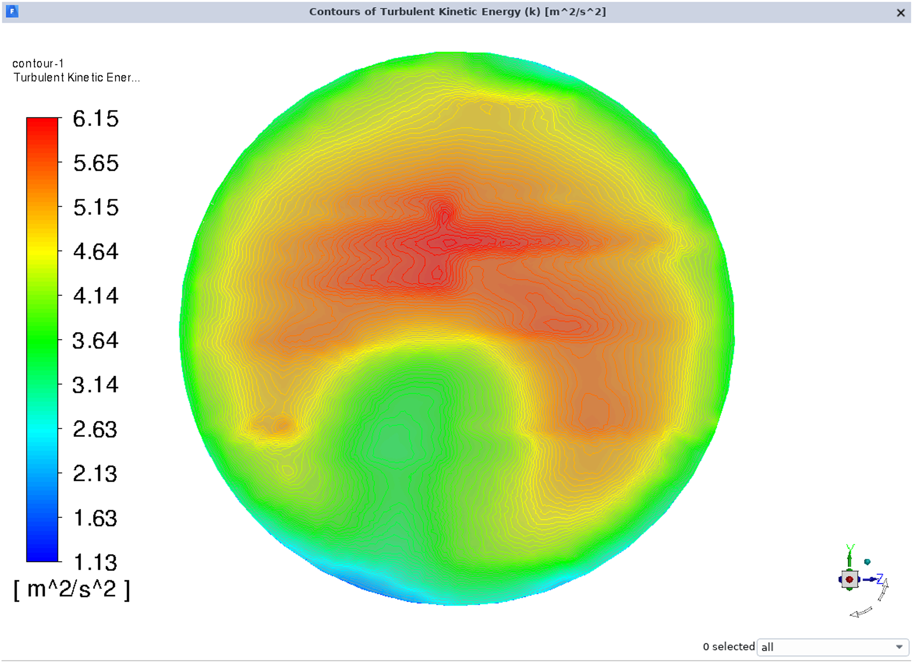
For the CFD model, two inlets were specified as shown in Figure 2. The velocity prescribed at the pipe inlet was taken from the interpolated values of the measurements, and the turbulent boundary condition prescribed was based on the hydraulic diameter of the pipe and turbulent intensity, which was measured to be 3.98%. Figures 5 and 6 show the velocity and k profiles at the pipe inlet, respectively.

Figure 5.

Measured velocity profile superimposed at the pipe inlet.

Figure 6.

Measured turbulent kinetic energy profile superimposed at the pipe inlet.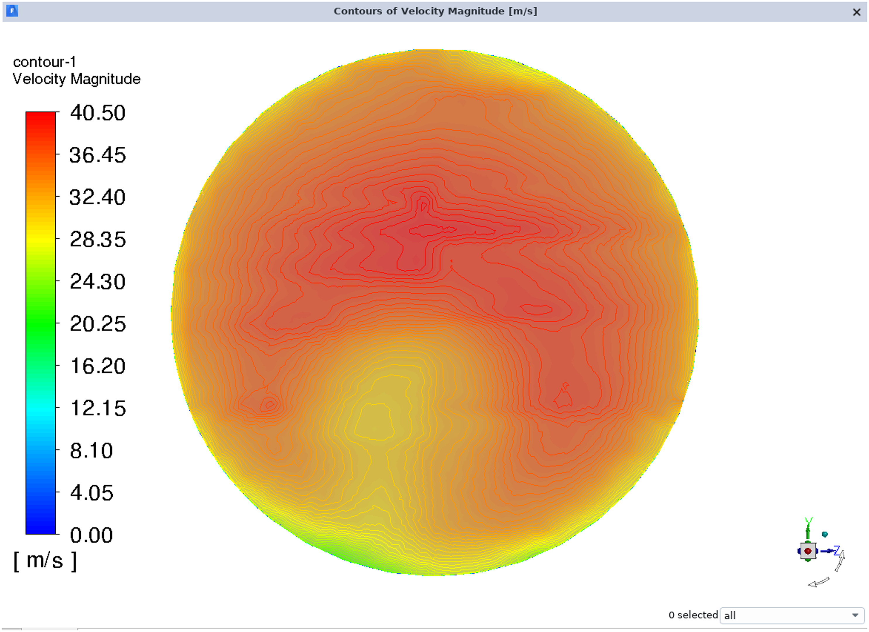

An outflow boundary condition was used at the outlet. Simulations were carried out using a coupled (pressure and velocity) solver with the psuedo-transient option enabled. The Least-Squares-Cell-Based method was chosen to compute gradients while the second-order upwind discretization scheme was selected for momentum. Upwind schemes were also selected for turbulent kinetic energy and dissipation rate. All surfaces apart from the two velocity inlets are modeled as no-slip walls.

Prior to the simulations, a mesh independence study was conducted with the SST k − ω model. The velocity profiles for three meshes were extracted at Plane 6 and compared, as shown in Figure 7. Mesh 1, Mesh 2, and Mesh 3 consisted of 42,050,255, 59,869,113, and 67,421,223 cells, respectively. Note that refinements in the mesh were in the region of the fuselage section. Slight differences were noticed in the velocity profiles between Mesh 1 and Mesh 2 while Mesh 2 and 3 demonstrated consistency between the profiles. Based on this result, Mesh 2 was selected for the study. For the subsequent simulations, four turbulence models, namely, the standard and realizable k − ϵ, SST k − ω, and Durbin’s model were used. The three ϵ-based turbulence models tested were simulated using scalable wall functions while the SST k − ω simulations ran with y⁺ ≈ 1 (Figure 7).

Figure 7.

Mesh independence study for Mesh 1, 2, and 3. Cell count for Mesh 1, 2, and 3 are 42,050,255, 59,869,113, and 67,421,223 hexacore cells, respectively.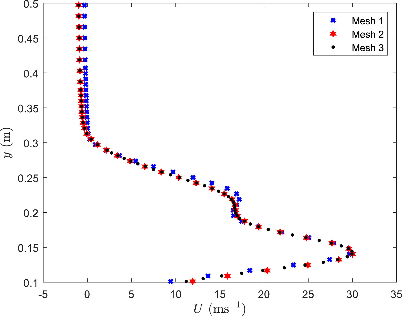

Results and discussion

The results discussed in this section will be on the first and sixth planes to capture the exhaust plume closest engine nozzle and further downstream with interactions, respectively. The experiments were split into flows without and with freestream velocity, designated as Case A and Case B, respectively. The freestream velocity U_e measured in Case B was 21 m/s and will be used as a normalization parameter for all velocities in this paper. All distances are normalized by the length of the cowling L = 1.5 m.

Case A: Plane 1

The normalized velocity magnitudes U/U_e are displayed in Figure 8 from both the PIV measurements and simulations for Plane 1 without freestream. y* and z* are vertical and spanwise distance normalized by L = 1.5 m, respectively. On first inspection, the general shapes of the cross-sectional plume predicted by all the turbulence models were congruent with the experiments. The measured plume exhibited a crescent-esque shape with two localized high speed regions. These local cores were identified as regions where U/U_e ≥ 2. All the models overpredicted the velocity within the plume with no distinct saddle points (local cores) as seen in the experiments. The spread of U/U_e ≥ 2 occupied the majority of the crescent for all turbulence models. The standard k − ϵ predicted less high speed regions and in this context, rendered it the more accurate model at this location. This model is normally accurate for flows where differences between rate of strain and rotation are negligible. The fact that the standard k − ϵ performed better than the other turbulence models suggests that there might not be large differences between strain and rotation at Plane 1 for Case A. Durbin’s model, which is a variant of the standard k − ϵ, overpredicted U/U_e the most within the plume.

Figure 8.

Case A plane 1: Comparison between measured and calculated normalized velocity magnitude. Velocity magnitude is normalized by U_e = 21 m/s. y* and z* are vertical and spanwise distance normalized by L = 1.5 m.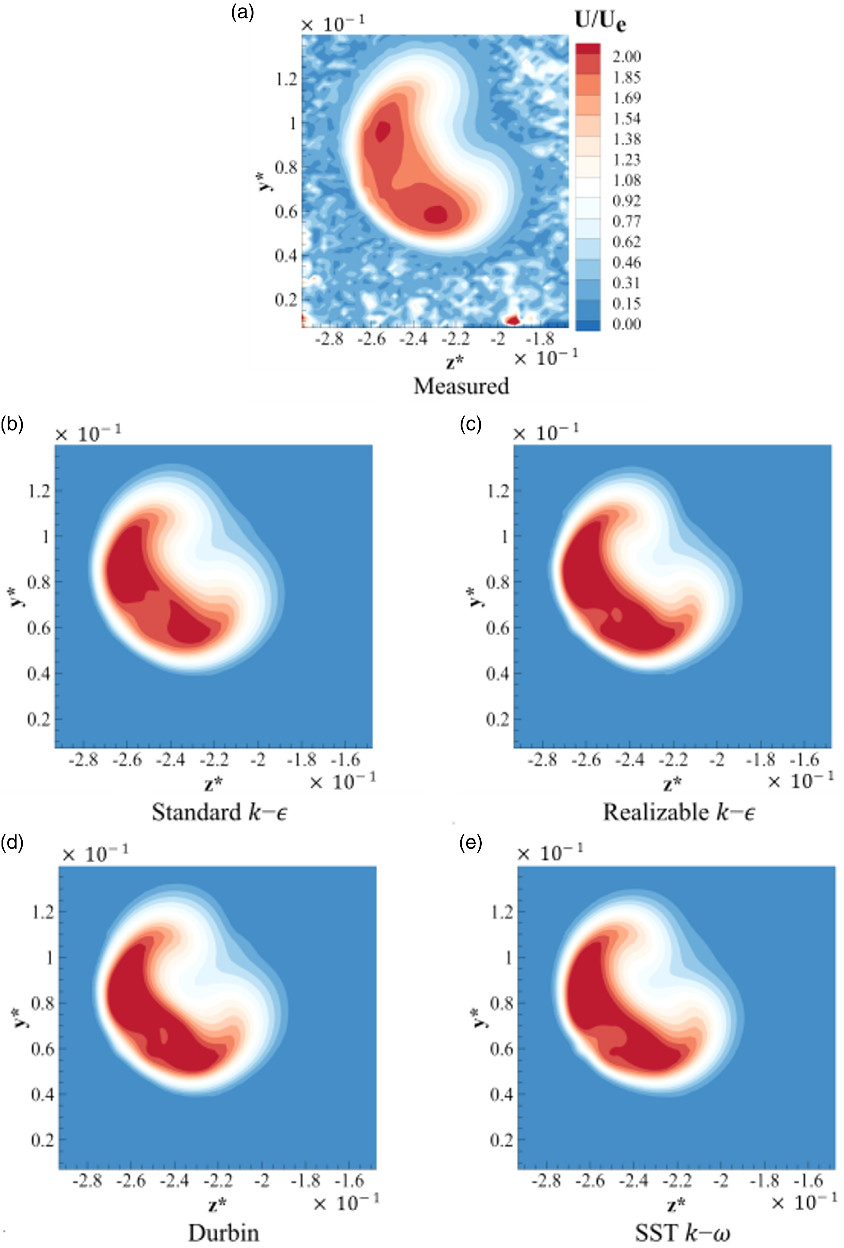

The vertical U/U_e profiles taken at z* = −0.23 (where it intersects the lower core from the experiments) are shown in Figure 9. The number of local U/U_e maxima and minima predicted by all models were in line with the experiments but these peaks do not match in terms of magnitudes and positions. At the lower core, in the region of 0.05 $\leq y^{*} \leq$ 0.06, all models overpredicted U/U_e with the standard k − ϵ coming the closest to matching the experiments. The measured peak at the lower core occurred at y* ≈0.058 while the standard k − ϵ produced a peak at y* ≈0.059 (Figure 9).

Figure 9.

Case A plane 1: Line profile of normalized velocity magnitude U/U_e at z* = −2.3 (Refer to 8).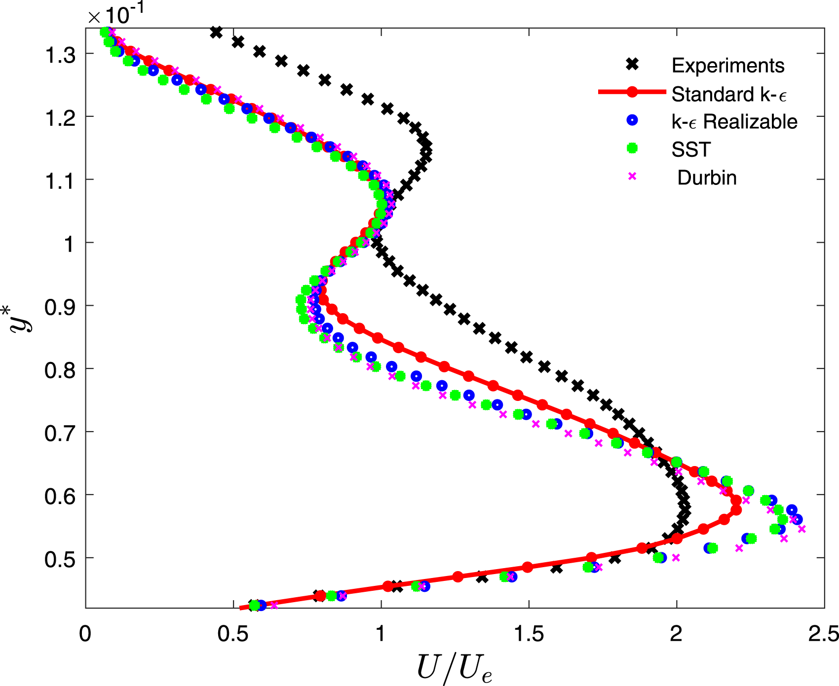

For the present analysis, the plume is the subject of interest and comparisons of arbitrary line profiles for velocities between models and experiments do not give a robust description of models’ performances for predicting plume shape and behavior. While the comparisons of contour plots provide an improved intuition, more information can be uncovered if these contours are allowed to be superimposed onto one another without causing too much confusion to the viewer. One way to do this is via the Principal Component Analysis (PCA).²⁶ PCA is a Data Science technique for dimensionality reduction,²⁶ and can be used to uncover low dimensional patterns in a system. The application to the present study involves first having to choose a certain range of velocities that defines the shape of the plume. Once these velocities are chosen, their coordinates are stored in a data matrix X with each row containing z* and y* (these are coordinates used in Figure 8). A scatter plot depicting the measured plume in Case A is shown in Figure 10. The normalized velocity selected for this particular case is U/U_e ≥ 0.92, chosen after a few trials and errors until the shape of the plume (represented mostly by the non-zero velocities) were captured (Figure 10).

Figure 10.

Case A plane 1: Scatter plot of measured plume with coordinates of U/U_e ≥ 0.92 considered.

The next step involves constructing a mean matrix $\bar{X}$ . This is done by first performing a column-wise summation of X, with the sum of each column $\bar{x_{j}}$ given as

\bar{x_{j}} = \frac{1}{n} \sum_{i = 1}^{n} x_{i j}

(1)where x_ij is the component in the ith row, jth column of X and n is the total number of coordinates with U/U_e ≥ 0.92. Here, j = 1, 2 as there are two coordinates, z* and y*. Subsequently,

\bar{X}

is then created by pre-multiplying the column-wise summation of X by a column vector of ones of length n. In line with PCA literature, the mean

\bar{X}

is then subtracted from X and stored in matrix C. The principal components can then be found using the Singular Value Decomposition (SVD) method.²⁷ The SVD of matrix C is

C = U_{r} Σ V^{T}

(2)

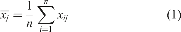
In order to delineate the distribution, a circle (which itself is a delineation of a Gaussian cloud) is first drawn with its center at $\bar{x_{j}}$ . The circle (where the angle θ extends from 0 to 2π) is then stretched and rotated by multiplying it by Σ and U_r (unitary matrix) from equation (2), respectively. The newly formed ellipse (also known as the confidence ellipse) captures one standard deviation of the data and is plotted in Figure 11. The first and second standard deviation confidence intervals are demarcated by the red and blue lines, respectively. For the remainder of the study, only the second standard deviation (95% confidence interval) will be used for comparisons between models and experiments. It should be made clear to the reader that the confidence ellipse occupies a region which covers the center of the distribution based on the chosen probability²⁸ and not 95% of the points.

Figure 11.

Case A plane 1: First (red) and second (blue) standard deviations of the confidence ellipses constructed via PCA.

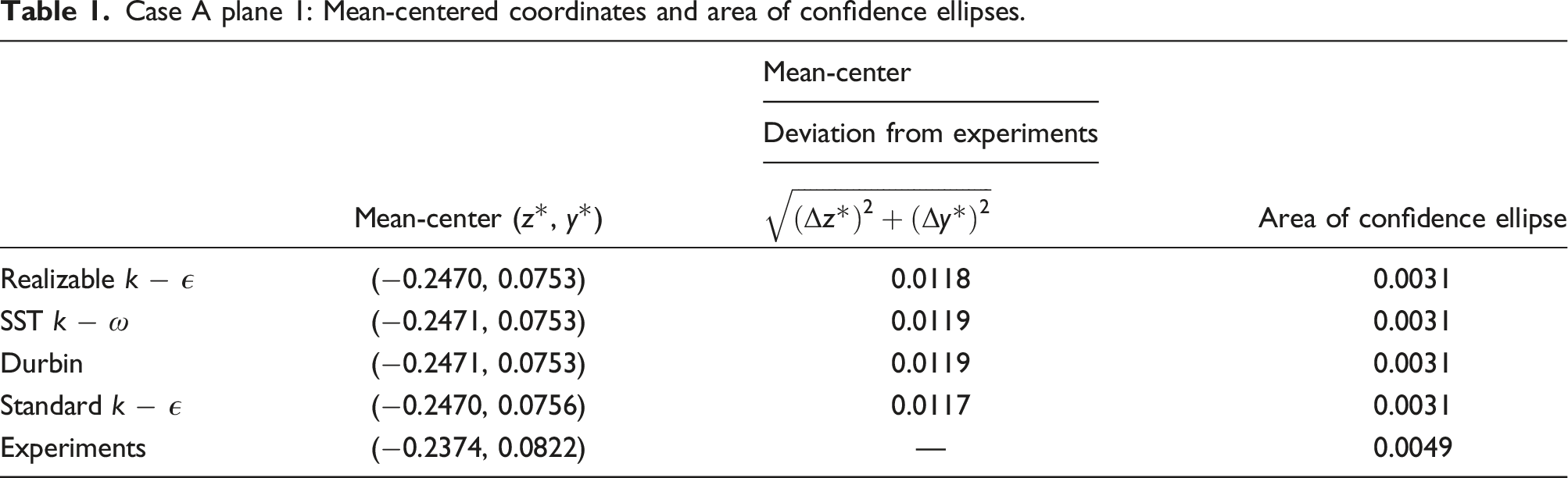
Figure 12 depicts the confidence ellipses representing the bivariate distribution of point cloud U/U_e ≥ 0.92 within the plume for both simulations and experiments. The measured plume scatter is shown at the inset. The models’ ellipses occupy a smaller region in the z*–y* plane as compared to the measurements. This is expected as the velocity distributions (within the plume) predicted by models in Figure 8 are mostly above U/U_e = 1.85. Small confidence ellipses relate to low variances (spread) of the distribution.

Figure 12.

Case A plane 1: Confidence ellipses for the simulations and experiments with distribution based on U/U_e ≥ 0.92. The scatter plot is based on the measured plume distribution.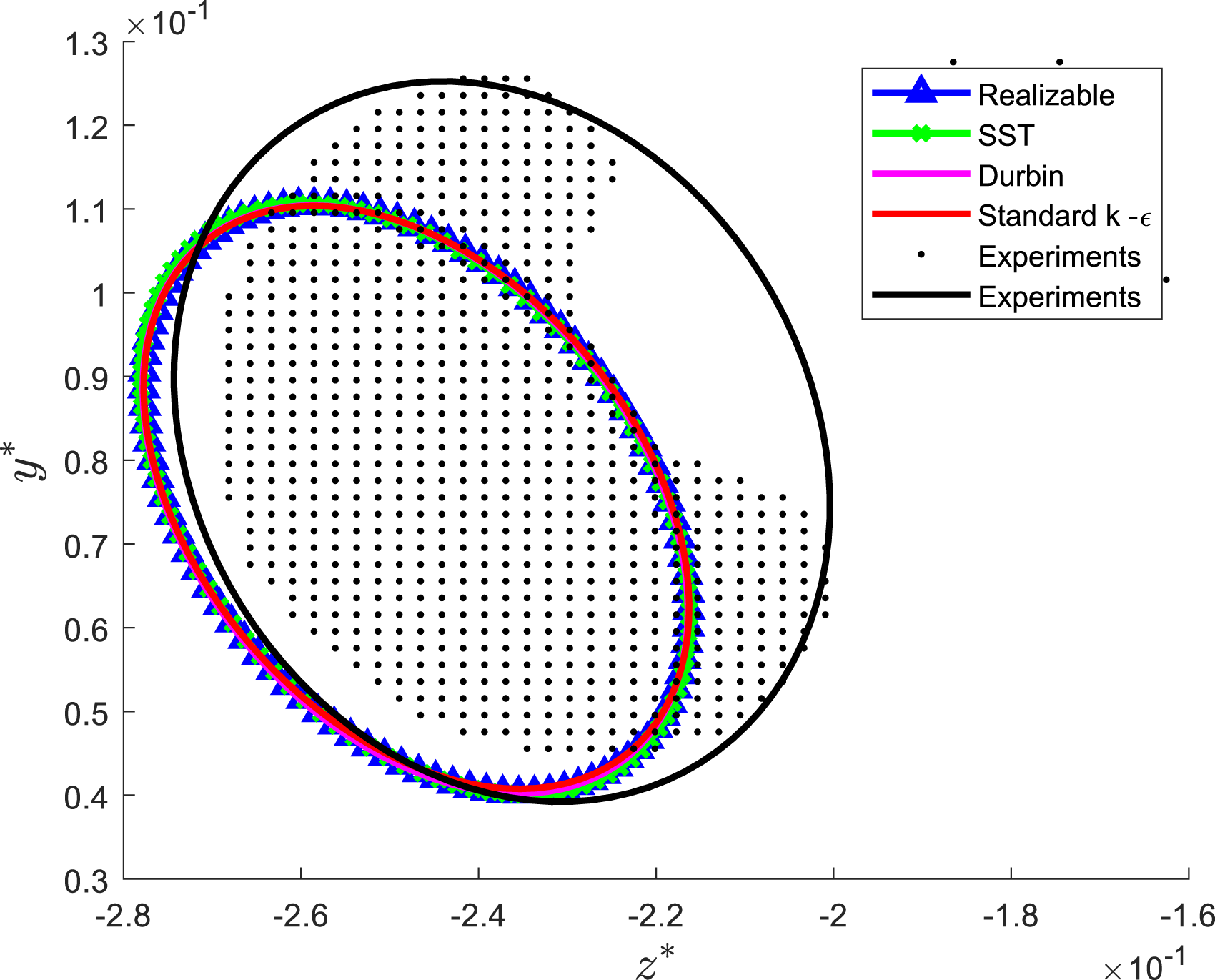

The fact that the measurements produced a more distended ellipse suggests that the range of velocities within the plume is more spread out. Interestingly, the turbulence models’ ellipses further demonstrated a shift in position (an offset in

\bar{x_{j}}

) and a tilt when compared to the experiments, which were not immediately obvious from the contour plots in Figure 8. The shifts in mean-centers, shown in Table 1, reveal that the standard k − ϵ came closest to matching the experiments, although it is fair to say that the rest of the models were not significantly different from the aforementioned model. The tilts of the confidence ellipses from the models are around 10° ∼ 11° from the experiments. As this is a bivariate distribution (z* and y*), there are two principal components, and this will be discussed shortly.

Table 1.

Case A plane 1: Mean-centered coordinates and area of confidence ellipses.

	Mean-center (z, y)	Mean-center	Area of confidence ellipse
		Deviation from experiments
		$\sqrt{{(Δ z^{})}^{2} + {(Δ y^{})}^{2}}$
Realizable k − ϵ	(−0.2470, 0.0753)	0.0118	0.0031
SST k − ω	(−0.2471, 0.0753)	0.0119	0.0031
Durbin	(−0.2471, 0.0753)	0.0119	0.0031
Standard k − ϵ	(−0.2470, 0.0756)	0.0117	0.0031
Experiments	(−0.2374, 0.0822)	—	0.0049

Case A: Plane 6

At plane 6 for Case A (Figure 13), the measured plume has diffused from its crescent shape at Plane 1 to an elongated billow. The two local cores earlier from Plane 1 are now stretched and are commensurate with both the losses and conservation of momentum, and synonymous with the observations made from Ref. 17. The simulations demonstrated the similar plume-stretching behavior but all models consistently predicted an anti-clockwise tilt (when viewed from the outlet) vis-à-vis the experiments.

Figure 13.

Case A plane 6: Comparison between measured and calculated normalized velocity magnitude. Velocity magnitude is normalized by U_e =21 m/s.

As with the observations at Plane 1, all the models overpredicted U/U_e within the plume. There is no surprise here as upstream errors are expected to propagate downstream. The overprediction suggests that with an improved prescribed velocity field at the pipe inlet (refer to Figure 2), predictions would come closer to matching the measurements for all models. As mentioned in the earlier section, Dean vortices from the pipe bend distort the flow so it is plausible to expect v and w momentum contributions (with u being the streamwise component). Note that in the experiments of Teo et al.,⁵ only one component of velocity (streamwise) was measured at the pipe inlet.

The contour plots from Plane 1 (Figure 8(c) and (d)) showed the realizable and Durbin models having a larger plume region filled with the highest velocity magnitude in comparison to the SST k − ω and standard k − ϵ. At Plane 6 from Figure 13(c) and (d), both the realizable and Durbin models showed two distinct cores of U/U_e ≥ 1.5, albeit occupying larger plume area relative to the experiments. The standard k − ϵ and SST k − ω showed no separation of plume region having U/U_e ≥ 1.5. It is safe to say that as the local cores attenuate, and with diffusion imminent, the plume dissipates. On that note, the SST k − ω results (Figure 13(e)) suggests the plume will maintain its shape as it advects downstream from Plane 6.

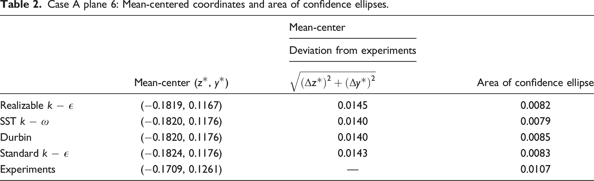
The confidence ellipses for Case A at Plane 6 are displayed in Figure 14. The distribution is based on the region covered by U/U_e ≥ 0.58. It is not surprising that the models’ ellipses have a tilt offset relative to the measurements as this was noticed earlier in the contour plots from Figure 13. The models’ tilts from the experiments are around 16° ∼ 17° anti-clockwise. The non-dimensionalized areas of the ellipses were calculated and shown in Table 2 to provide a sense of the variance in the data since it is difficult to tell from visual inspection alone. While the models’ areas are close to the same size to each other (0.0079–0.0085), they fall short of the measurements’ area of 0.0107.

Figure 14.

Case A plane 6: Confidence ellipses for the simulations and experiments with distribution based on U/U_e ≥ 0.58. The scatter plot is based on the measured plume distribution.

Table 2.

Case A plane 6: Mean-centered coordinates and area of confidence ellipses.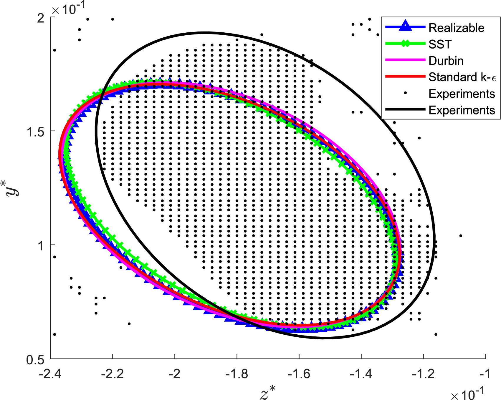

	Mean-center (z, y)	Mean-center	Area of confidence ellipse
		Deviation from experiments
		$\sqrt{{(Δ z^{})}^{2} + {(Δ y^{})}^{2}}$
Realizable k − ϵ	(−0.1819, 0.1167)	0.0145	0.0082
SST k − ω	(−0.1820, 0.1176)	0.0140	0.0079
Durbin	(−0.1820, 0.1176)	0.0140	0.0085
Standard k − ϵ	(−0.1824, 0.1176)	0.0143	0.0083
Experiments	(−0.1709, 0.1261)	—	0.0107

The principal components computed from equation (2) are ordered. That is to say, with two dimensions, Σ produces an ordered 2×2 diagonal matrix. The first principal component (the larger of the two) from Σ points to the direction along which variance is the largest. The second principal component is orthogonal to the first and maximizes the variance based on that orthogonality. Figure 15 displays the principal components for Planes 1 and 6 for Case A. The arrows denote the first principal components for models and experiments while the vectors without arrows represent the second principal components. The mean-centers for the models have been shifted to the experiment’s centers for clarity.

Figure 15.

Case A: Principal components of the ellipses from experiments and simulations, for planes 1 and 6. The arrow heads represent the first principal components while the vectors without arrows are the second principal components.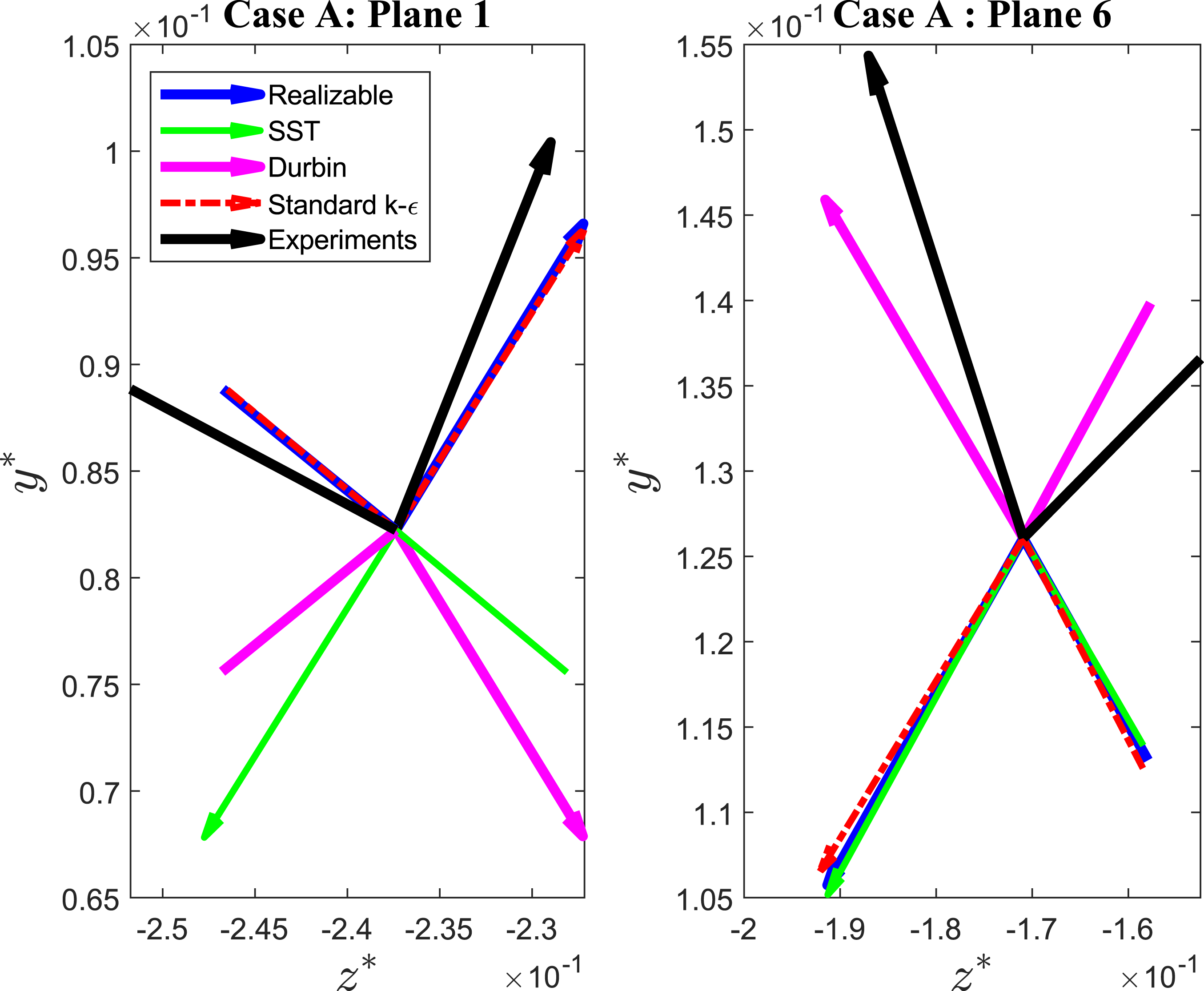

For Plane 1, the realizable and standard k − ϵ first principal components came closest to matching the experiments’ in that the projection of the variance is maximum in the first quadrant of their plumes (based on z* and y*). The SST k − ω and Durbin models showed that their first principal components are in the third and fourth quadrant, respectively. It is taken note in passing that the simulations for Case A did not reproduce the plume distributions accurately (possibly due to an ill-prescribed velocity flow field at the pipe inlet). It is thus put forth that if advection is the dominant term among the production, diffusion and dissipation of turbulence, the errors would be expected to attenuate. The basis for this argument rests on the fact that the advection term is explicit. That is to say it is not modeled unlike the Reynolds stresses via the eddy viscosity. The results presented in the next set of paragraphs are for Case B (in freestream conditions).

Case B: Plane 1

Figure 16 portrays the measured and simulated U/U_e at Plane 1 for Case B. It is interesting to note that the measured plume is not only elongated when compared to Case A at Plane 1 in Figure 8(a), but it appears to have flipped about its axis (the direction of the fold in the crescent-shaped plume for Case A favors the side away from the cowling). This predilection for the particular direction is due to the plume’s interaction with the boundary layer off the cowling. Although all the models managed to capture the essence of the plume, the intensity was not well-predicted for lower y* values. In fact, while the measurements infer significant fluid entrainment at the lower bounds of the core, the models showed flatter and weaker lower tails in the region of 0.02 ≤ y* ≤0.03. If the predicted lower tail is of any indication of a model’s accuracy, then the SST k − ω is the least accurate among the four models.

Figure 16.

Case B plane 1: Comparison between measured and calculated normalized velocity magnitude. Velocity magnitude is normalized by U_e = 21 m/s.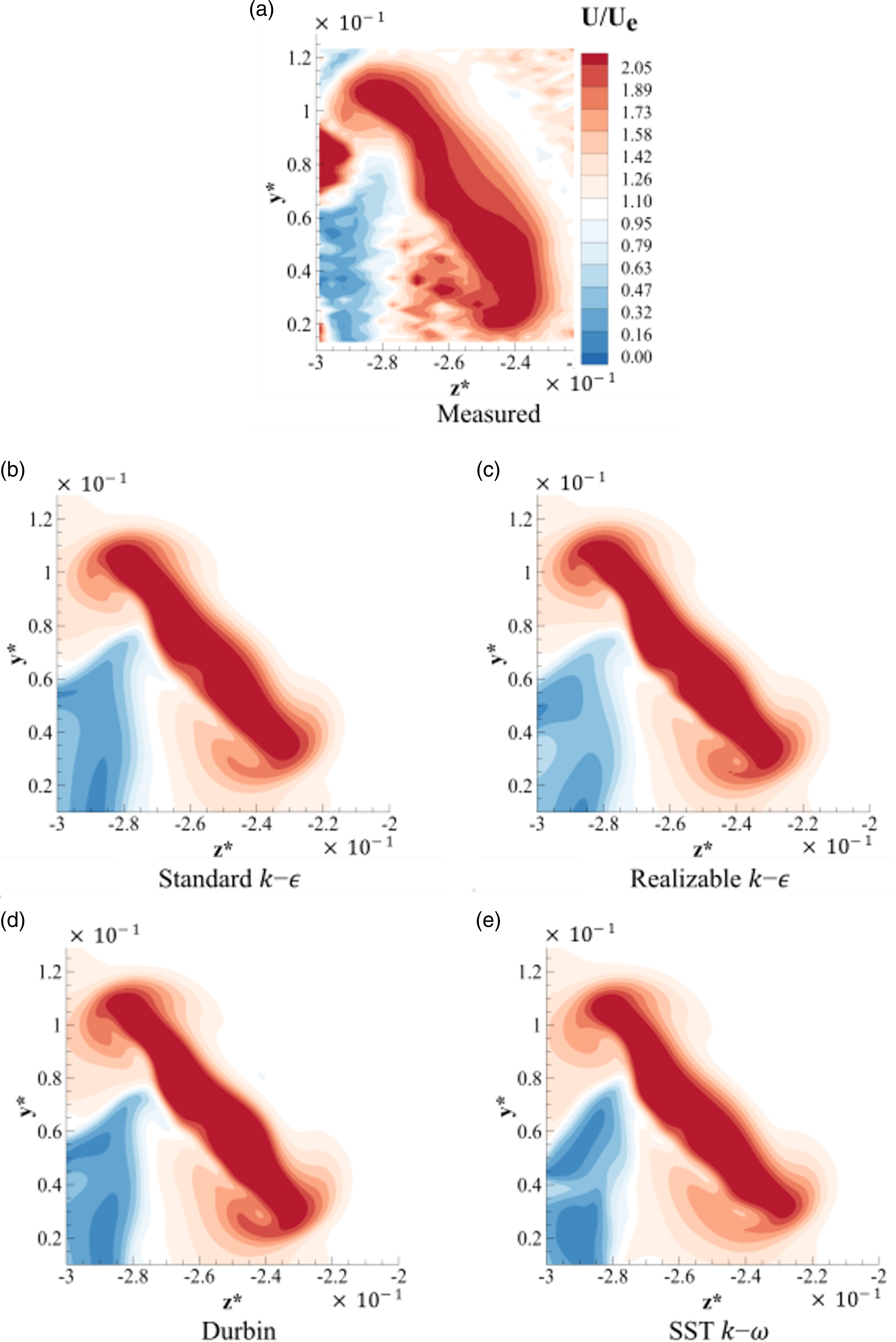

For a more robust yardstick of models’ performances, the confidence ellipses were plotted for Plane 1 and displayed in Figure 17. As with Case A, the selection of U/U_e was based on a series of trials and errors until the shape of the plume was reasonably captured. At Plane 1 for Case B, the values of U/U_e ≥ 1.73 were selected for the population. It can be inferred from Figure 17 that the simulations do not have a large dispersion of the population as compared to the experiments. This is mainly due to the region near the lower tail of the measured plume where a few “intense” spots were observed (in the region below y* = 0.04 and −0.27 $< z^{*} <$ 0.24 in Figure 16(a). Table 3 shows the large variation between the measurements’ and simulations’ ellipse areas. Although the models’ predicted mean-centers are an improvement from Case A at Plane 1, the analysis of this nature (low dimensionality) outlines its sensitivity. This is despite the fact that the essence of the plume is captured by all the models, as shown qualitatively in Figure 16.

Figure 17.

Case B plane 1: Confidence ellipses for the simulations and experiments with distribution based on U/U_e ≥ 1.73. The scatter plot is based on the measured plume distribution.

Table 3.

Case B plane 1: Mean-centered coordinates and area of confidence ellipses.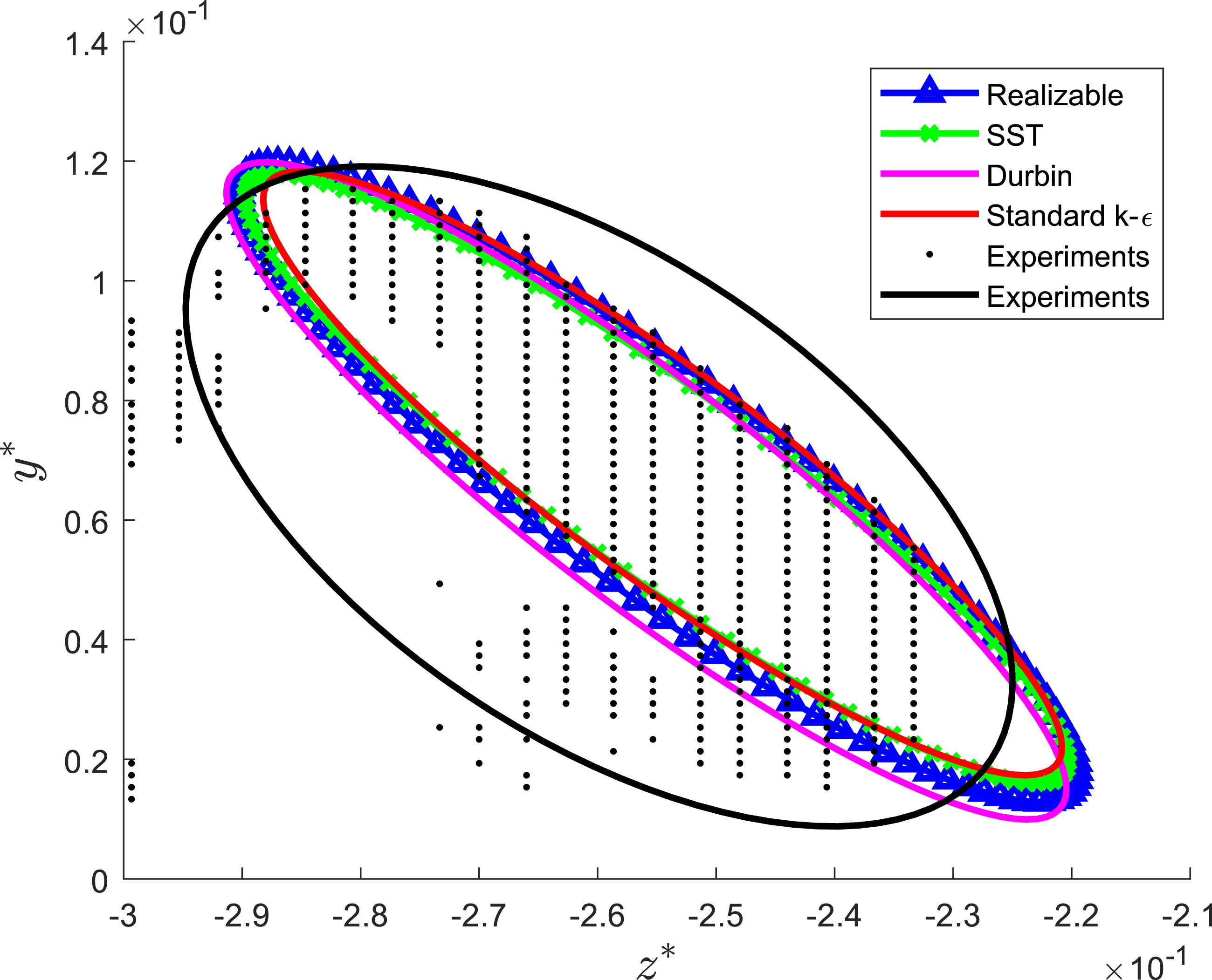

	Mean-center (z, y)	Mean-center	Area of confidence ellipse
		Deviation from experiments
		$\sqrt{{(Δ z^{})}^{2} + {(Δ y^{})}^{2}}$
Realizable k − ϵ	(−0.2548, 0.0662)	0.0056	0.0025
SST k − ω	(−0.2550, 0.0670)	0.0057	0.0021
Durbin	(−0.2559, 0.0649)	0.0041	0.0026
Standard k − ϵ	(−0.2545, 0.0678)	0.0066	0.0022
Experiments	(−0.2599, 0.0640)	—	0.0050

Case B: Plane 6

The results at Plane 6 for Case B is perhaps the most important in the experiments if the main objective is to look at the impingement of the exhaust gases on the tail boom of a helicopter. The measured plume at Plane 6 for Case B shown in Figure 18(a) appears to have risen and this is expected given the inclined angle of the exhaust on the body (see Figure 1). The plume at this location is less intense than the one seen at Plane 1, which strongly suggests it has lost much of its streamwise momentum (either through diffusion or gains in vertical and spanwise momentum). Interestingly, the plume has coiled inwards and this could be due to its interaction with a recirculation zone (possibly immediately after the exhaust tube). The simulations captured the main shape of the plume at Plane 6 albeit the difference in distribution of velocities predicted by each model. The measurements reveal that the local U/U_e maxima occurs in the center of the coil at 0.05 $< y^{*} <$ 0.1. The realizable k − ϵ captured this feature of the plume the best among the models although, like all models, it overpredicted the velocity magnitude in the lower part of the coiled plume. Another feature of the measured plume is the hook-like flow structure at the end of its path (at 0.07 $< y^{*} <$ 0.085). From the simulations, while not entirely accurate in terms of velocity distribution, Durbin’s model predicted the most profound “hook.”

Figure 18.

Case B plane 6: Comparison between measured and calculated normalized velocity magnitude. Velocity magnitude is normalized by U_e = 21 m/s.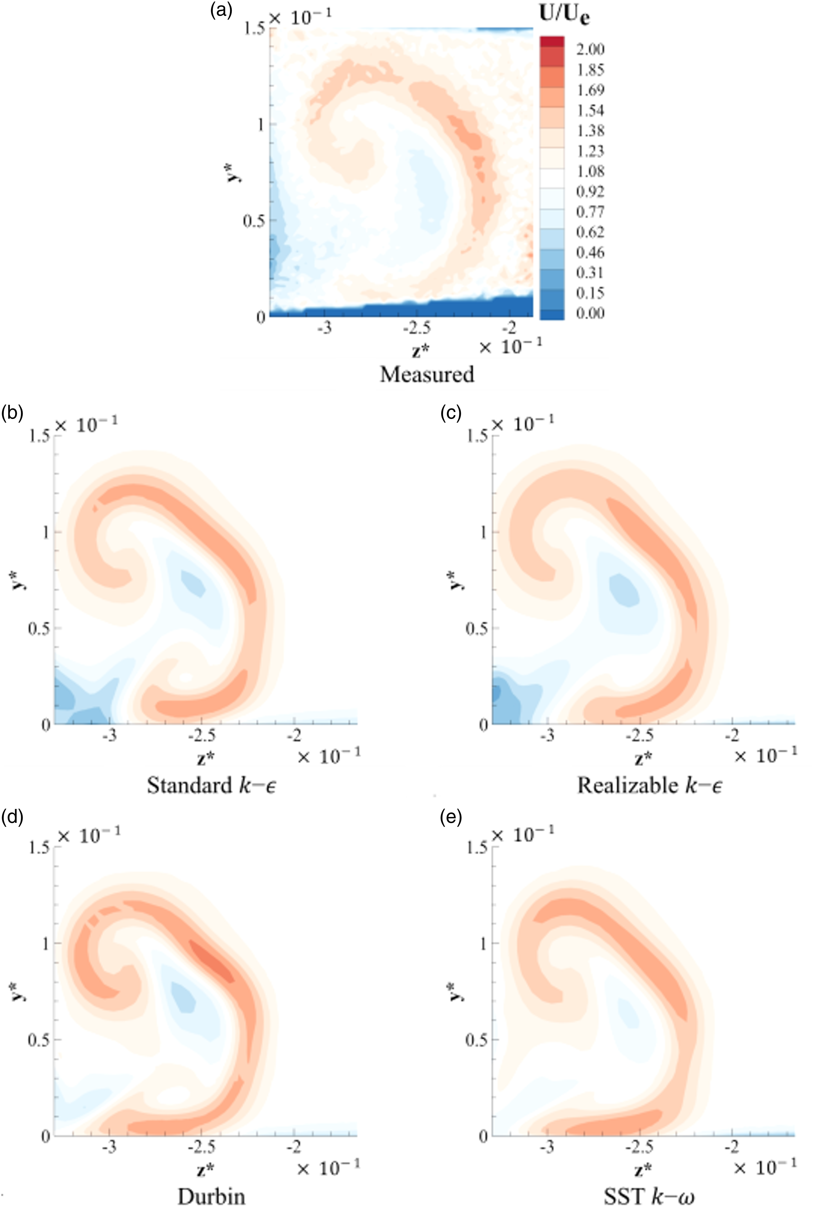

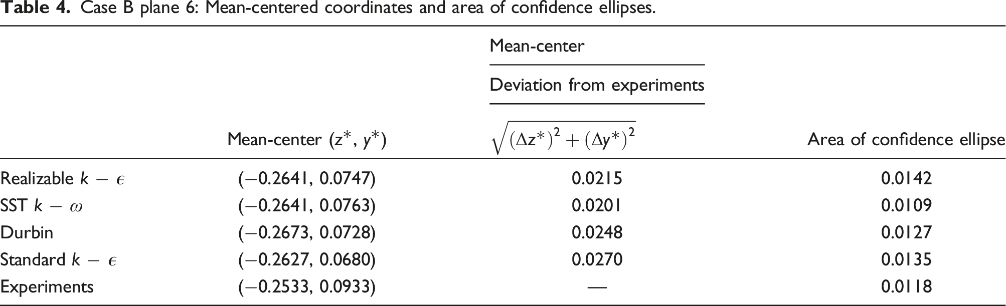
The confidence ellipses for Case B at Plane 6 are shown in Figure 19. The distribution was based on the plane having U/U_e ≥ 1.2. This is the most interesting among all the ellipses plotted previously because the plot shows visible variations between the models. In terms of the statistical variance, all models barring the SST k − ω showed a larger spread when compared to the experiments. The areas for all ellipses and their mean-centers are tabulated in Table 4. Although all simulations managed to capture the main shape of the plume at Plane 6 for Case B, their ellipse mean-centers are shifted towards the direction of negative z* (towards the cowling).

Figure 19.

Case B plane 6: Confidence ellipses for the simulations and experiments with distribution based on U/U_e ≥ 1.2. The scatter plot is based on the measured plume distribution.

Table 4.

Case B plane 6: Mean-centered coordinates and area of confidence ellipses.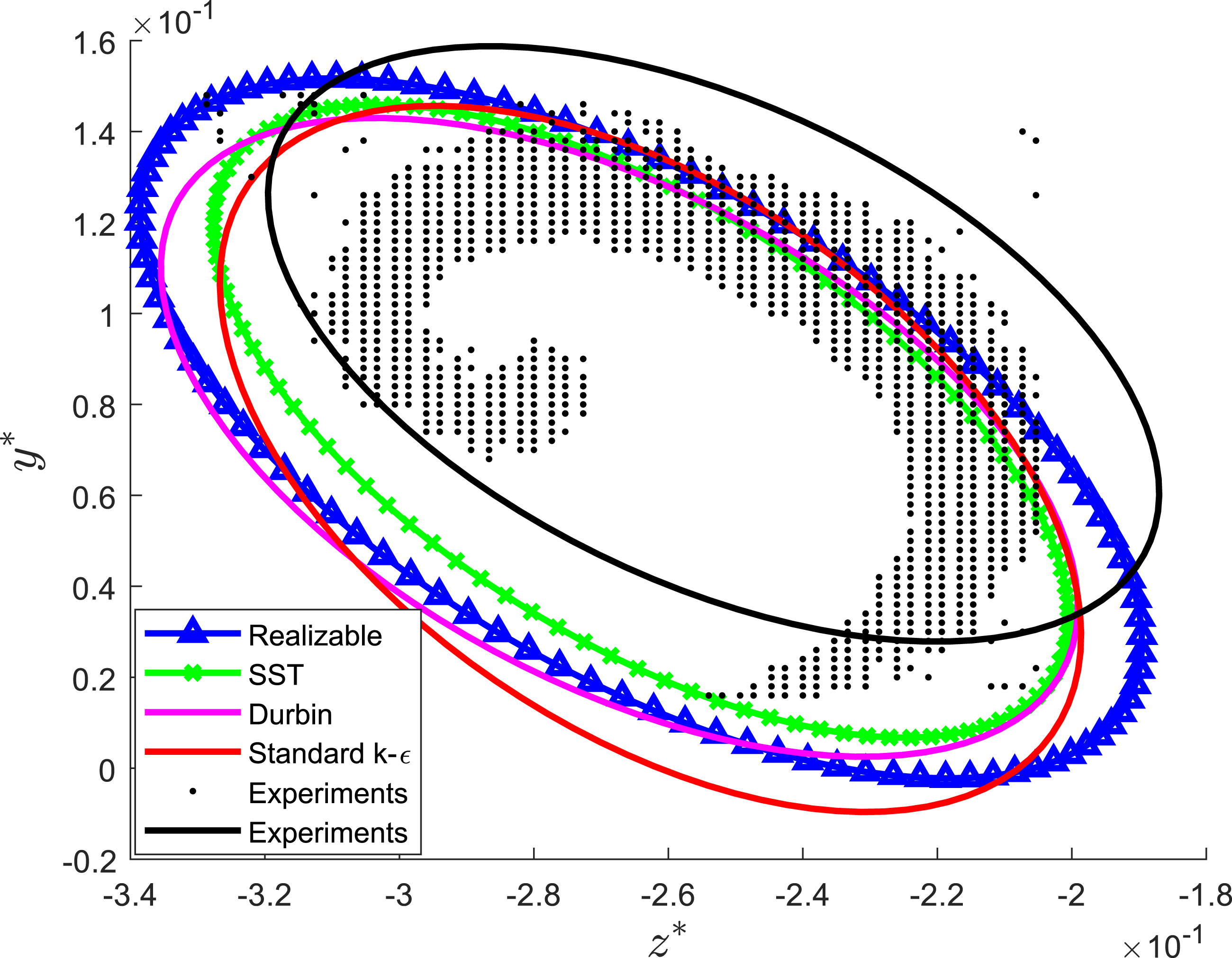

	Mean-center (z, y)	Mean-center	Area of confidence ellipse
		Deviation from experiments
		$\sqrt{{(Δ z^{})}^{2} + {(Δ y^{})}^{2}}$
Realizable k − ϵ	(−0.2641, 0.0747)	0.0215	0.0142
SST k − ω	(−0.2641, 0.0763)	0.0201	0.0109
Durbin	(−0.2673, 0.0728)	0.0248	0.0127
Standard k − ϵ	(−0.2627, 0.0680)	0.0270	0.0135
Experiments	(−0.2533, 0.0933)	—	0.0118

Apart from Plane 1 for Case B, the direction of the shifts is consistent for the two planes analyzed. Note that at Plane 1 for Case B, the experiments’ ellipse’s positioning was influenced by the velocity blobs below y* ≤0.05 (see Figure 16(a)). It is interesting to note that the qualitative assessment from Figure 18 concluded with the realizable k − ϵ being one of the more accurate models but Table 4 shows that it has the largest spread among the models with an ellipse area of 0.0142. The SST k − ω model’s ellipse area is the only one that is smaller than the experiments. If the differences in ellipse areas are compared for Case A and Case B at Plane 6 (refer to Table 5), then it can be concluded that models’ errors are reduced when freestream velocity is present. The results shown in Table 5 are encouraging given the fact that the lack of information for the boundary condition at the pipe inlet (v and w velocity components) will not generally affect the plume shape and distribution in the presence of freestream velocity.

Table 5.

Differences in models’ ellipse areas in comparison with experiments.

	Case A (%)	Case B (%)
Realizable k − ϵ	23.36	20.34
SST k − ω	26.17	7.63
Durbin	20.56	7.63
Standard k − ϵ	22.43	14.41

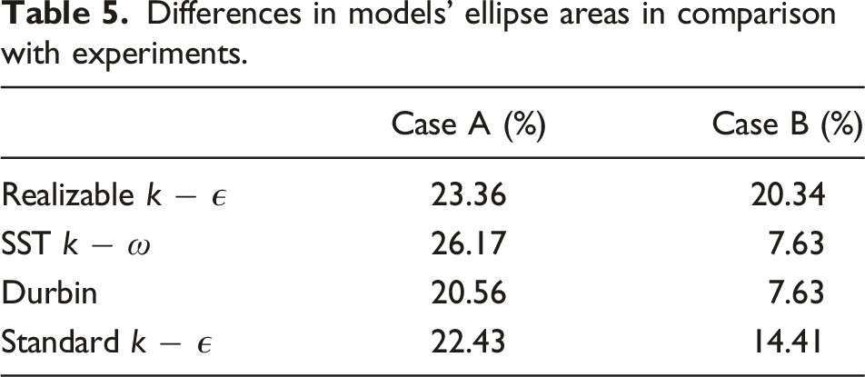
The principal components computed for Case B for the experiments and simulations are presented in Figure 20. As with Case A, the mean-centers of the models are shifted to match the experiments for clarity. At Plane 1 for Case B, the experiments showed that the largest variance (the first principal component) is projected in southwest direction. Only Durbin’s model came closest to matching this projection. This is not to say that it managed to capture the experiments’ velocity “blobs” in the southwest projection (refer to Figure 16(a)). Rather the model has larger velocity variations, relative to the other models, at the ends of the predicted plume at Plane 1 in Figure 16(d). At Plane 6 for Case B, the larger variances pointed out by the first principal component was predicted most accurately by the realizable k − ϵ model. Note that this was in the direction pointing to the hook-like feature of the measured plume seen in Figure 18. The standard k − ϵ also came close to matching the direction of the first principal component while Durbin and the SST k − ω showed that the maximum variance of the plume occurred northeast of their mean-centers. Based on the area of the ellipse at Plane 6, it appears that the SST k − ω and Durbin’s model are the most accurate.

Figure 20.

Case B: Principal components of the ellipses from experiments and simulations, for planes 1 and 6. The arrow heads represent the first principal components while the vectors without arrows are the second principal components.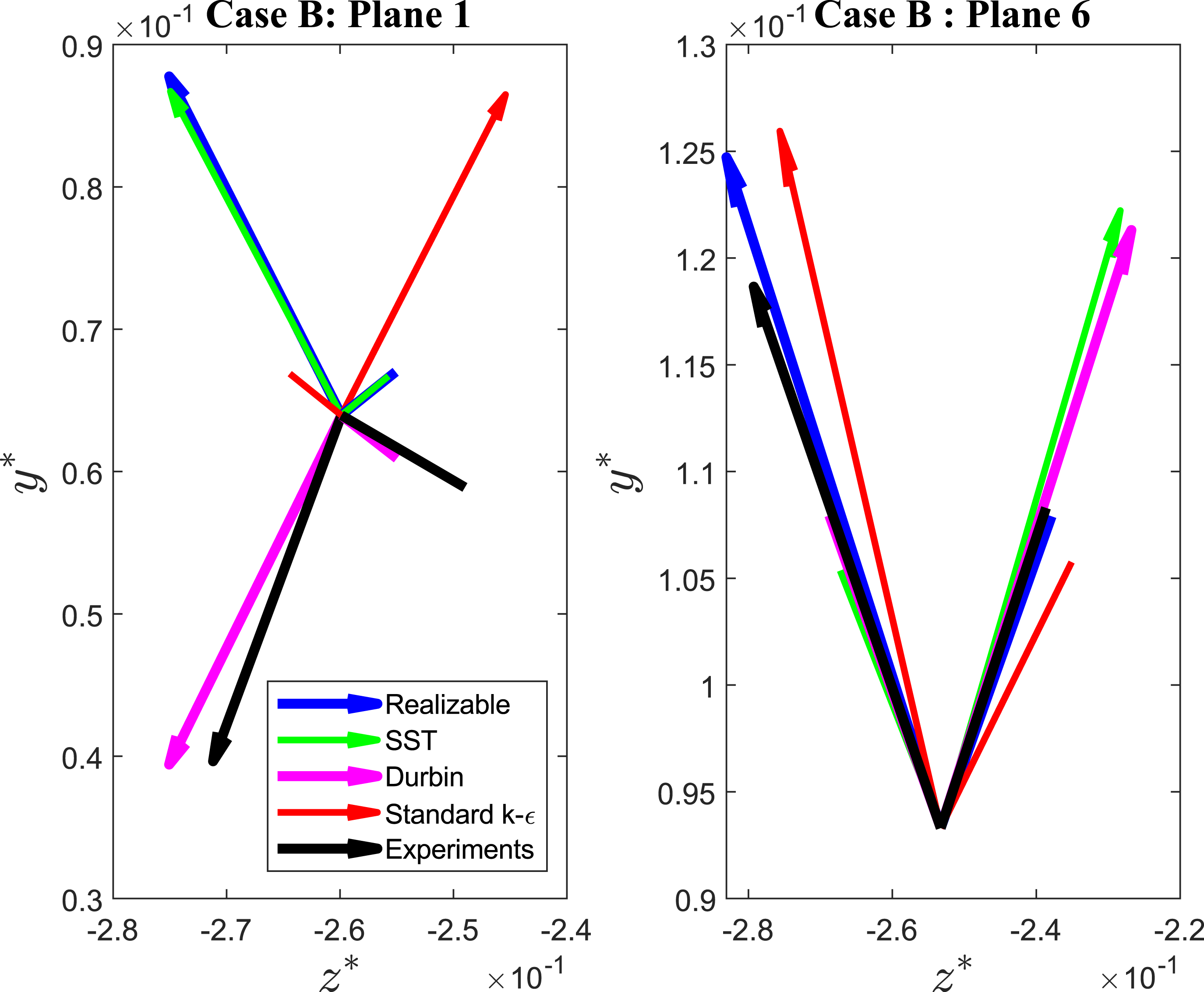

Conclusions

Four turbulence models were tested for a simulated flow of a helicopter exhaust to compare their performances on capturing the flow behavior of the resulting plume. They were the standard and realizable k − ϵ models, Durbin’s model and the SST k − ω. For the two freestream-to-exhaust velocity ratios of 0 (Case A) and 0.6 (Case B), all models managed to capture the general shape of the measured plume at two measurement stations from qualitative assessments via the comparisons of velocity magnitude contours at two planes. While velocity line profiles can quantify the comparisons, there are no precepts for suitable locations to describe the plume.

Through PCA, confidence ellipses of the plume distribution (both experiments and simulations) were computed, and the results were superimposed onto one plot. This strategy allows for the proper assessment of the models’ prediction of plume distribution relative to that of the velocity magnitude contours. The models’ confidence ellipses all showed a shift in position in comparison to the experiments. The shifts could be the due to lack of information pertaining to the v and w velocity components at the pipe inlet. The locations of the maximum statistical variance (first principal component) for the plume distribution were then extracted from the PCA calculations. It was shown that for Case A at Plane 1 and 6, the models showed a smaller variance in terms of plume distribution when compared to experiments. The reverse is true for Case B for all models except the SST k − ω at Plane 6. It was also found that with freestream, errors of the models reduced, and this is important as it is representative of actual flight conditions. The most important results are at Plane 6 as this was the furthermost measuring station. In terms of matching the measured plume shape for the no-freestream case, all models showed that they were capable of matching the general shape of the plume. It was observed however that at lower y* values, the models failed to replicate the experimental velocity distribution. Durbin’s model exhibited the best match to the experiments in terms of plume shape in freestream conditions at Plane 6. In terms of plume deviation from experiments, computed via comparisons of confidence ellipses, the SST k − ω deviated the least in freestream conditions.

Footnotes

Declaration of conflicting interests

The author(s) declared no potential conflicts of interest with respect to the research, authorship, and/or publication of this article.

Funding

The author(s) disclosed receipt of the following financial support for the research, authorship, and/or publication of this article: The authors acknowledge the support provided for this study by Leonardo-Finmeccanica Helicopter Division.

ORCID iDs

Tze How New

Bing Feng Ng

References

Teo

Wong

Lee

, et al. Characteristics of helicopter engine exhaust through scaled experiments using stereoscopic particle image velocimetry. Proc Inst Mech Eng, Part G: J Aerosp Eng 2020a; 235(9): 1091–1104. In-press.

Conlisk

. Modern helicopter aerodynamics. Annu Rev Fluid Mech 1997; 29(1): 515–567.

Zhang

Pan

Shan

. Progress in helicopter infrared signature suppression. Chin J Aeronaut 2014; 27(2): 189–199.

Knoth

Breitsamter

. Flow analysis of a helicopter engine side air intake. J Propul Power 2017; 33(5): 1230–1244.

Teo

Wong

Mohamed

, et al. On the flow measurements of simulated helicopter exhausts. In: AIAA Scitech 2020 Forum. Orlando, FL, 2020b. p. 2226.

Götten

Havermann

Braun

, et al. Wind-tunnel and CFD investigations of UAV landing gears and turrets–improvements in empirical drag estimation. Aero Sci Technol 2020; 107: 106306.

Le Chuiton

. Actuator disc modelling for helicopter rotors. Aero Sci Technol 2004; 8(4): 285–297.

Shi

, et al. Numerical investigation on the ship/multi-helicopter dynamic interface. Aero Sci Technol 2020; 106: 106175.

Launder

Spalding

. The numerical computation of turbulent flows. In: Numerical prediction of flow, heat transfer, turbulence and combustion, 1983. pp. 96–116.

10.

Durbin

. On the k-ɛ stagnation point anomaly. Int J Heat Fluid Flow. 1996; 17(1): 89–90. doi:10.1016/0142-727X(95)00073-Y

11.

Koutmos

McGuirk

. CFD predictions of lobed mixer performance. Comput Methods Appl Mech Eng 1995; 122(1–2): 131–144.

12.

Menter

. Zonal two-equation k-ω turbulence models for aerodynamic flows. In: 23rd fluid dynamics, plasmadynamics, and lasers conference, 1993. p. 2906.

13.

Menter

. Two-equation eddy-viscosity turbulence models for engineering applications. AIAA J 1994; 32(8): 1598–1605.

14.

Fogaing

MBT

Hemmati

Lange

, et al. Performance of turbulence models in simulating wind loads on photovoltaics modules. Energies 2019; 12(17): 3290.

15.

Stokkermans

Veldhuis

Soemarwoto

, et al. Breakdown of aerodynamic interactions for the lateral rotors on a compound helicopter. Aero Sci Technol. 2020; 101: 105845. doi:10.1016/j.ast.2020.105845

16.

İper

Ergin

Cenik

, et al. Investigation of the effects of lobe number and configuration on mixing performance in lobed mixer. In: AIAA Propulsion and Energy 2020 Forum, 2020. p. 3778.

17.

McCormick

Bennett

Jr . Vortical and turbulent structure of a lobed mixer free shear layer. AIAA J 1994; 32(9): 1852–1859.

18.

Dettleff

. Plume flow and plume impingement in space technology. Prog Aero Sci. 1991; 28(1): 1–71. doi:10.1016/0376-0421(91)90008-R

19.

Biava

Khier

Vigevano

. CFD prediction of air flow past a full helicopter configuration. Aero Sci Technol 2012; 19(1): 3–18.

20.

Spalart

Allmaras

. A one-equation turbulence model for aerodynamic flows. In: 30th Aerospace Sciences Meeting and Exhibit. Reno, NV, 1992. p. 439.

21.

Durbin

Reif

. Statistical theory and modeling for turbulent flows, vol. 2. Hoboken, NJ; Wiley Online Library, 2001.

22.

Knoth

Breitsamter

. Aerodynamic characteristics of helicopter engine side air intakes. Aircraft Eng Aero Technol 2018; 90(9): 1355–1363.

23.

Dean

. XVI. Note on the motion of fluid in a curved pipe. London, Edinburgh Dublin Phil Mag J Sci 1927; 4(20): 208–223.

24.

Shaw

Wilson

. Wind tunnel investigation of simulated helicopter engine exhaust interacting with windstream. Techreport NASA TM X-3016. Hampton, VA: NASA Langley Research Center, 1974.

25.

Kyrkos

Ekaterinaris

. Assessment of an unstructured mesh approach for CFD predictions of the NH90 fuselage rotor. Aero Sci Technol 2012; 19(1): 77–85.

26.

Pearson

. Principal components analysis. London, Edinburgh Dublin Phil Mag J Sci 1901; 6(2): 559.

27.

Brunton

Kutz

. Data-driven science and engineering: machine learning, dynamical systems, and control. Cambridge: Cambridge University Press, 2019.

28.

Rocchi

MBL

Sisti

Ditroilo

, et al. The misuse of the confidence ellipse in evaluating statokinesigram. Ital J Sport Sci 2005; 12(2): 169–172.

On the numerical assessment of engine exhaust plumes with a scaled cowling