
Abstract
This paper aims at presenting a novel monocular vision–based approach for drones to detect multiple type of weeds and estimate their positions autonomously for precision agriculture applications. The methodology is based on classifying and detecting the weeds using a proposed deep neural network architecture, named fused-YOLO on the images acquired from a monocular camera mounted on the unmanned aerial vehicle (UAV) following a predefined elliptical trajectory. The detection/classification is complemented by a new estimation scheme adopting unscented Kalman filter (UKF) to estimate the exact location of the weeds. Bounding boxes are assigned to the detected targets (weeds) such that the centre pixels of the bounding box will represent the centre of the target. The centre pixels are extracted and converted into world coordinates forming azimuth and elevation angles from the target to the UAV, and the proposed estimation scheme is used to extract the positions of the weeds. Experiments were conducted both indoor and outdoor to validate this integrated detection/classification/estimation approach. The errors in terms of misclassification and mispositioning of the weeds estimation were minimum, and the convergence of the position estimation results was short taking into account the affordable platform with cheap sensors used in the experiments.
Keywords
Introduction
Agriculture as a whole provides a means of livelihood ranging from food production, pharmaceuticals, textiles and raw materials for industries. However, the productivity of this sector is threatened by the existence of weeds which are parasitic in nature. 1 Weeds are unwanted plants that grow on the farmland and compete with the desired plants for water, nutrients, space and sunlight. The losses in productivity reach 25% in Europe, but in the less developed areas in Africa and Asia, almost half of the potential food yield is lost due to weeds. 2 It is reported that lettuce yield is reduced over 50% due to weeds, 3 wheat yield is reduced by 15% 4 and there is up to 71% drop in seeded tomato yield 5 due to weed infestation.
Conventionally, weeds are removed using crude tools and herbicides. However, these processes are wasteful and dangerous to the environment since these herbicides are made of harmful chemicals. To efficiently remove weeds, there is a need to carefully identify the weed, then localize its exact position and then finally apply the right quantity of the herbicides or deploy the appropriate tool for the weed removal. This gives rise to the consideration of robotics platforms for weed removal. While some works have proposed mechanical robotic tools,1,6 others proposed robotic sprayers to reach the objective.7–10
Weeds can be identified using computer vision techniques.1,11 The adoption of deep neural networks (DNNs) for weed detection is increasing.12–14 To bridge the gap between weed detection and precise weed removal, this paper addresses the problem of identification and localization of the weeds.
Commercially available systems for smart weed detection and removal are generally expensive. The availability of affordable off-the-shelf unmanned aerial vehicles (UAVs) with essential sensors makes it pertinent to exploit them for this research. The fusion of the information from several sensors through a robotics operating system (ROS) 15 makes it possible to perform several complicated tasks through effective communication between the sensors. Works such as navigation, 16 path planning 17 and localization of targets 18 have been possible through this set-up. Thus, we seek to exploit an affordable platform for this work and extend the solution scope to localizing and estimating the relative position of the weed.
In this paper, a Parrot AR drone platform is subjected to a predefined elliptic trajectory, and the stream of images from a monocular camera mounted on it are acquired throughout its motion. The stream of images are utilized to precisely detect the object of interest in the images using a deep detection network. The used network is a cascaded ResNet-50 19 and YOLOv4. 20 The detected weeds are then assigned to bounding boxes, and the centre pixels of the assigned bounding boxes are extracted. A centre pixel is assumed to be the centre of the detected weed, and it is transformed from image frame to world coordinates. Azimuth and elevation angles of the target centre point with respect to the are extracted and later fused in the unscented Kalman filter (UKF) 21 to estimate the location of the weed. The contributions of the paper are twofold: (1) utilizing an affordable platform equipped with a monocular camera for accurate multiple target position estimation and (2) extending the use of a DNN output beyond detection and identification to relative position estimation such that the information obtained from the detection network (bounding boxes, region of interest pixels) can be further processed to achieve relative position estimation of the detected target.
The paper continues with a literature review in the next section. The simulation and experimental frameworks are discussed in the subsequent sections. The results are demonstrated and discussed in the final sections.
Literature review
Weed detection using feature extraction in image processing is the earliest technique used to identify weeds with computer vision. Edge detection has been utilized as a technique for weed detection.22,23 However, the main plant and weed cannot be effectively differentiated using edge detection only. Different illumination conditions can be used to improve the detection using a colour model and split component of gray images. 7 A vertical projection method and a linear scanning method are combined to quickly identify the centre line of the crop rows. However, in this method, it is assumed that every plant detected outside the centre line of the crop rows is a weed. This is not always the case as weeds can also grow along the centre line. Machine learning techniques provided results that perform better if weeds are not on the centre line of the crop rows.13,24 Nevertheless, all these methods are not capable of precisely detecting the exact specie of weed. These limitations prompted the use of DNN for weed detection.
Weed detection was performed for perennial rye-grass with deep learning convolutional neural network. 14 The work concluded that VGGNet 25 performed better with the rye-grass dataset. This performance can be improved by capturing sequential information and combining RGB and NIR images. 26 The drawback to this work is again the lack of weed specie detection for accurate herbicide selection. Another work investigated the combination of classification and detection for fruits. 12 Similarly, in our previous work, we combined a classification and detection network for weed detection. 27 This way, we can categorically tell the type of weed and identify a region of interest (ROI) for further processing.
The accuracy of weed detection can be impacted by many factors such as variable lighting condition, sun angles, occluded and damaged plant leaves, and changing morphological or spectral properties of plant leaves at different growth stages. 28 It becomes imperative to use a rich dataset for training with different conditions. The conventional four steps in the procedure for using ground-based machine vision and imaging processing techniques in weed detection are the pre-processing, segmentation, feature extraction and classification. 29 We aim at extending this procedure to localizing and estimating the relative position of the weed.
The crowded literature on target localization can be grouped according to the platform used,30,31 or the sensors employed18,32 or the estimation model studied.31,33 The main aim for all is to maximize the localization accuracy and minimize the time required. Few however seek to use small UAVs with affordable sensors to achieve a high performance. A combination of 2D laser range finder with a monocular camera can be used for the localization. 30 Although the maximum deviation recorded using this method was about 13% from the actual measurement. This may be due to the not so robust target detection process employed in the paper. Edge detection and colour detection were utilized to detect the only green circular target in the scene. In reality, there can be many targets with seemingly similar features. Moreover, using this approach to detect the target while in flight can cause target blurring. An alternative approach was presented based on real-time kinematic positioning and thermal imagery. 33 This approach is based on the assumption that as long as a ground rover and a base station maintain at least 5 satellites in common, there can be an accurate prediction of the rover’s location.
The first to exploit the combination of UAV state estimates with the image data to acquire bearing measurements of the target and utilizing them in the target localization is Ponda et al. 34 In their work, a fixed wing UAV was subjected to numerous trajectories to find the optimal trajectory for target localization. The image data of the target are processed to obtain bearing angles from the drone to the target, and an extended Kalman filter (EKF) is used for position estimation. Even though it is a simulation work, good estimation results were obtained after 50 measurements for a single target. Another work also attempted the estimation with a fixed wing UAV and using a recursive least squares (RLS) filter but suffered a wide error of 10.9 m. 31 To tackle the limitations of fixed wing UAV particularly in manoeuvrability and altitude of flight, a quad-rotor can be used. 31 Accurate results were obtained after 30 seconds for a single target using this method.
Methodology
Problem definition
The problem is to estimate the exact position of the weed using a UAV with no sophisticated sensors. An affordable platform equipped with monocular camera with no sufficient information such as depth being generated makes it difficult to estimate the positions of weeds relative to the platform. The idea is to utilize the camera to detect a target and utilize the detection bounding boxes to estimate the target’s position. To do so, first the platform identifies/detects and localizes the target in the image frame. We used our trained network for the target detection and performed some post-processing to localize the target in the image frame. Second, the information from bounding boxes are used to estimate the centre position in the image frame. Since the objective is to reach a solution with a monocular camera set-up, where the depth information is not readily at hand as in the case of a stereo camera set-up, we converted the bounding box’s centre pixels to bearing angles and afterwards into azimuth and elevation angles (further explained in the Technical and Theoretical Approach section) with respect to the UAV. Thus, our problem can be divided into (1) acquiring the images from a monocular camera and transferring them to the ground station together with the position of the UAV, (2) detection and classification of the weed from a monocular camera, (3) extracting the position of the weed in the image frame and (4) estimating the position of the weed in the world frame. In order to have an accurate estimate for world coordinates of the weed, measurements regarding this information should be rich. The UAV is controlled to make a predefined ellipse trajectory. The nature of the trajectory is an important factor of the estimation accuracy as the field of view (FOV) varies from one point to another along the trajectory. Since the targets are at a stationary position, we try to limit the FOV of the camera to cover all the targets at each point along the trajectory so that we can obtain updates from each target simultaneously. A constant trajectory altitude at 1 m is selected. The bearing angle measurements for the position of the weed are fused in a UKF framework.
Technical and theoretical approach
The solution approach is summarized in a process flow chart shown in Figure 1. The process flow encompasses mainly the data acquisition section, and the ROS nodes on the ground station and the output section. The input data acquisition section is the hardware that provides inputs to the system. The image stream from the monocular camera mounted on the drone, and the ground truth positions of the UAV and the target (weed) measured by the tracking system are the inputs to the process. The ROS nodes hosted on a ground station with core-i7 processing power are the main processing part of the system. Detection and classification of the weed using a DNN, centre pixel extraction on the images, calculating the bearing angles, fusing the bearing angles to estimate world coordinates of the weed with UKF and the trajectory planning with drone driving tasks are performed on the ROS nodes. The output section consists of position coordinates of the estimated target (weed). Solution architecture.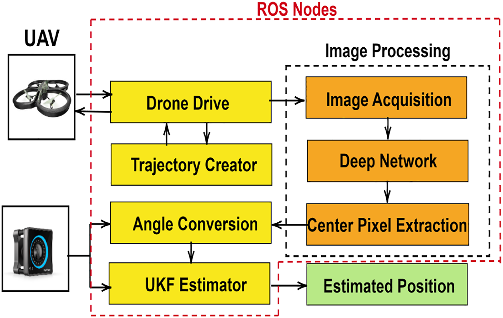
Unmanned aerial vehicle and tracking system
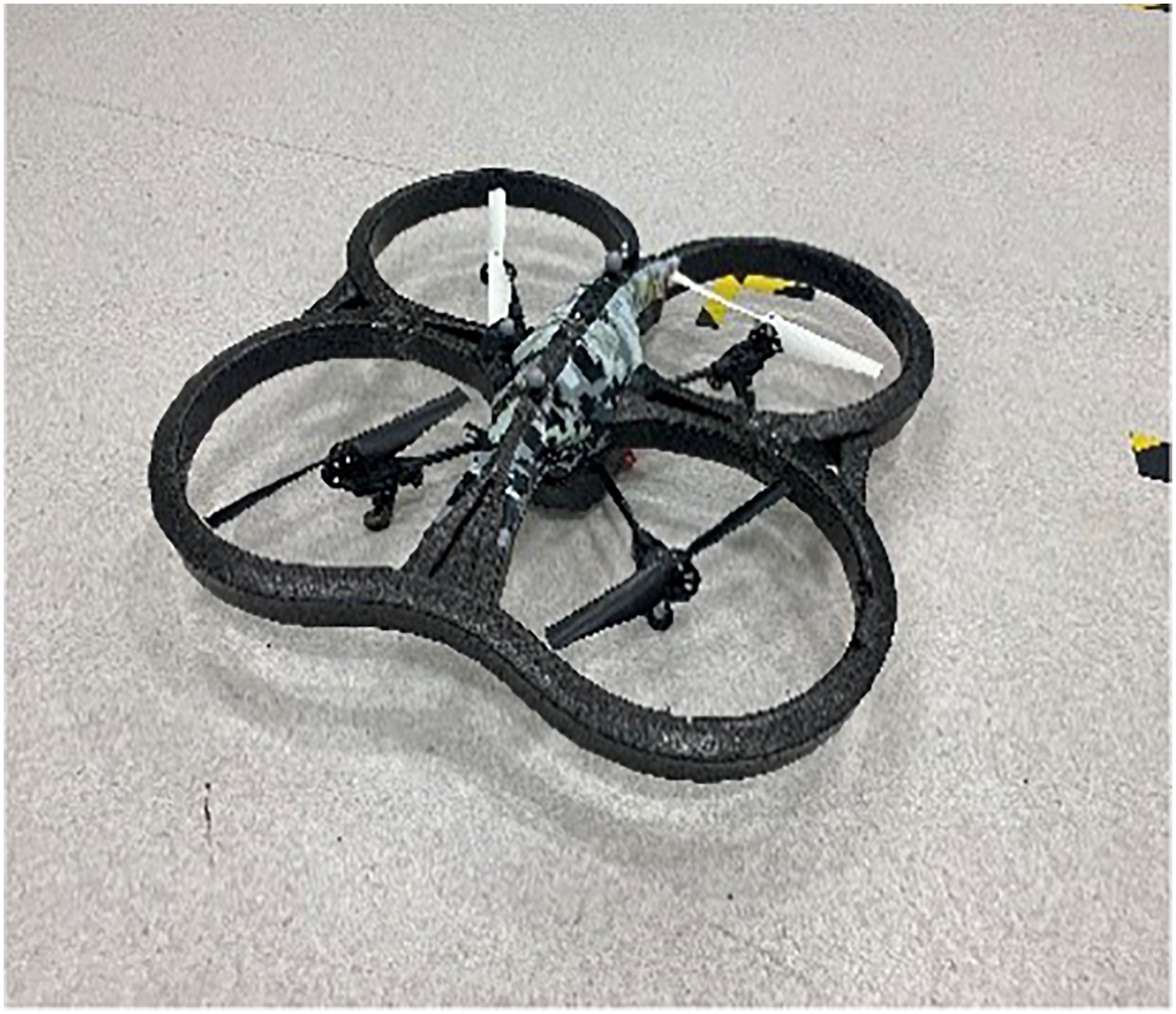
The UAV used is an affordable off-the-shelf Parrot AR drone. It is a six degree-of-freedom quadcopter with a miniaturized IMU, an ultrasonic sensor, a frontal camera with 720p sensor and 93° lens, a downward/vertical camera with QVGA sensor with 64° lens and 4 brushless 14.5 watt, 28.500 RPM in-runner type motors. 35 The tracking system is a set of cameras with 1.3 MP resolution, +/−0.30 mm 3D accuracy, 240 frames per second (FPS) native frame rate and 1000 FPS max frame rate which are used for tracking. 36
Drone driver
The drone driver is a ROS package that consists of all the libraries of the Parrot drone’s sensors and inbuilt controllers. We utilize the drone driver to control the drone and also to receive image feeds from the drone’s camera. The planar velocity references in UAV frame

Trajectory creator
This node provides the profile of trajectory to be performed by the drone and updates the drone driver with the necessary control parameters for following this trajectory. In this work, an ellipse trajectory is employed taking inspiration from the circular proposed for target localization.
8
We modified this to an ellipse so that the neighbouring targets can fit into the FOV. The trajectory profile is defined as follows
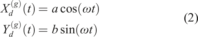
Therefore
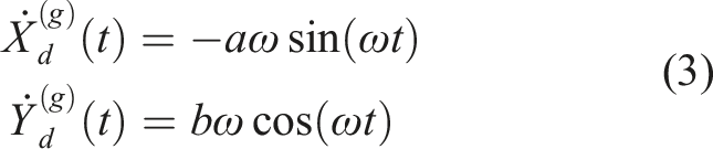
Image acquisition
This node receives image data from the drone driver and distributes to the detection network via an image transport link. Images are transported in the form of messages at a frequency of 200 Hz so they can effectively be utilized by the detection network. The drone’s camera was calibrated beforehand and the parameters were obtained.
Deep network
Conventionally, approaches such as colour detection or edge detection are deployed for weed detection problem.18,37 Most of the time, weeds have about 90% resemblance with the main plant. To contain this, a DNN is used to detect the weeds, similar to our previous work 27 but with modifications to suit this peculiar problem. The network is a cascade of a classification network ResNet-50 and a detection network YOLOv4. A detection network is necessary since using a classification network alone will classify the entire image as a weed which includes the ROI and the background without categorically indicating the weed within the image. In this paper, it is required to know the region within the image that corresponds to the weed. The choice of ResNet-50 as the classification network is pertinent to the work of the accuracy obtained in fruit classification. 12 YOLO framework was selected since the speed of detection for this network is almost twice as fast as two-staged detectors in weed detection. 27 This architecture is 95%–98% effective in weed classification and detection. 27 The network was trained with a dataset of 2000 images of the weed obtained form. 38
The DNN used for this work is shown in Figure 2. The final layers of the ResNet-50, namely, average pooling layer, fully connected layer, softmax and classification layers were truncated and merged with a YOLOv4 network. The final activation layer of the ResNet-50 was utilized as the feature extraction layer of the YOLOv4 so that the activation layer becomes the input to the YOLOv4. In the rest of the paper, this architecture will be referred as fused-YOLO. Fused-YOLO deep neural network architecture.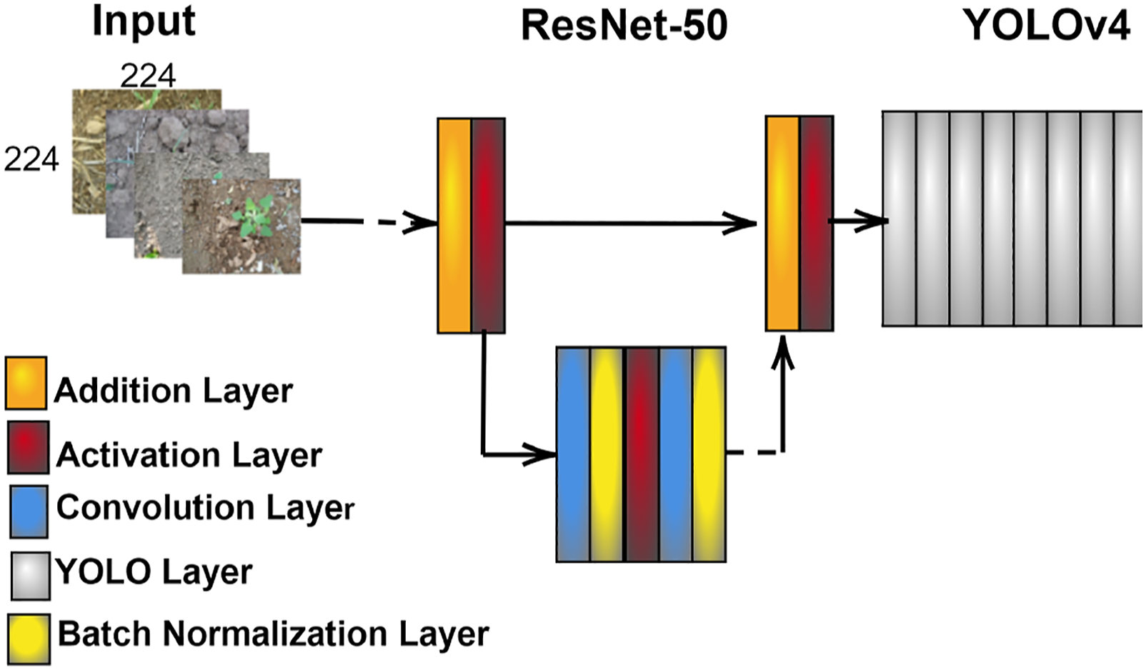
The input layers of the trained network are not compatible with the output coming from the drone camera. An encoding–decoding operation was performed as shown in Figure 3 to remap and rearrange the pixels. Encoding–decoding of images.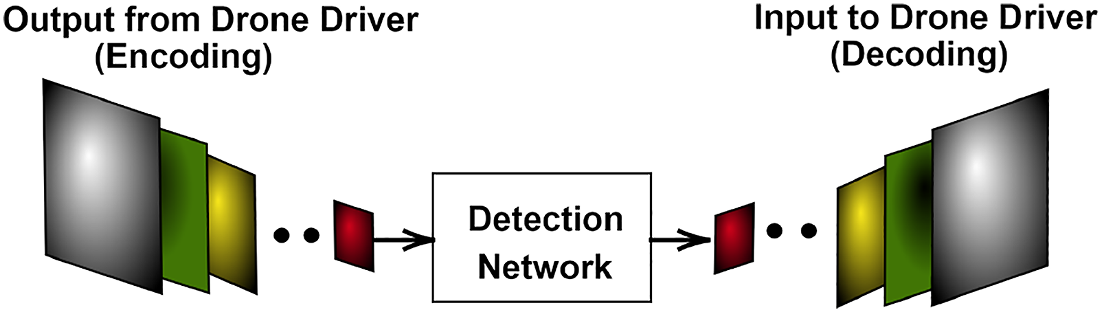
The encoding–decoding process was done to rearrange all the pixels from the drone camera to fit into the input layer of the fused-YOLO. The fused-YOLO receives images from the image acquisition node as input, the targets/weeds are detected and a bounding box is assigned for each weed detected as seen in Figure 4. Bounding box extraction. 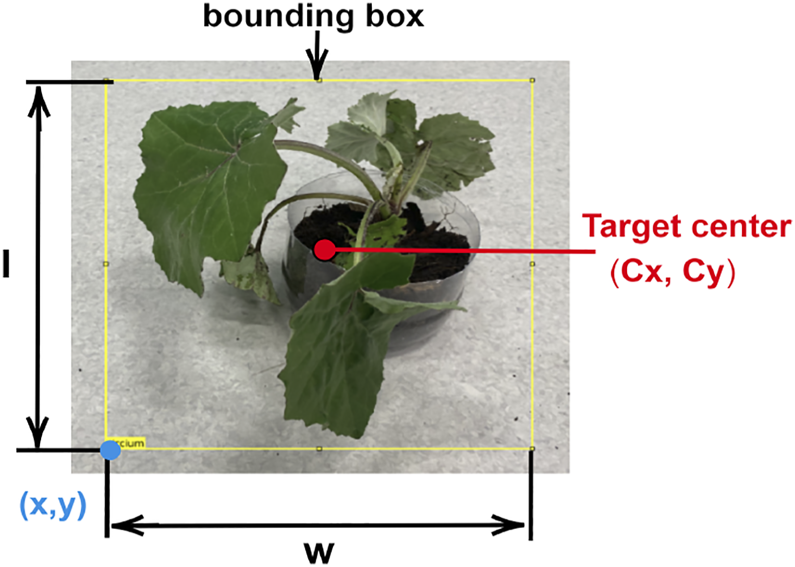
Centre pixel extraction
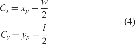
After each detection, the centre pixel of the detection bounding box is extracted. It is assumed that the centre of the bounding box coincides with the centre of the weed whose position is to be estimated as in Figure 4. This location in the image frame is converted to world coordinates as the geometric centre of the weed
Calculation of bearing angles
Provided the frontal camera orientation and pointing axis are known, using the Parrot drone on-board inertial measurement unit (IMU) and the odometry information, the centre pixels are converted to bearing angles ( Image projection figure where Obtained azimuth and elevation angles 
Unscented Kalman Filter estimator
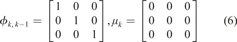
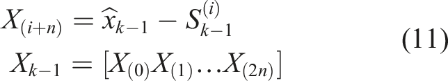
As the drone follows a prescribed trajectory, different bearing measurements for the position of the target are acquired, and these measurements are fused in a UKF framework. The nonlinearity in the azimuth and elevation measurements (
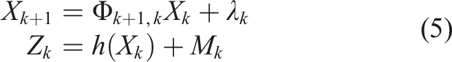
Here,
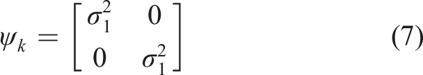
The measurement covariance matrix is
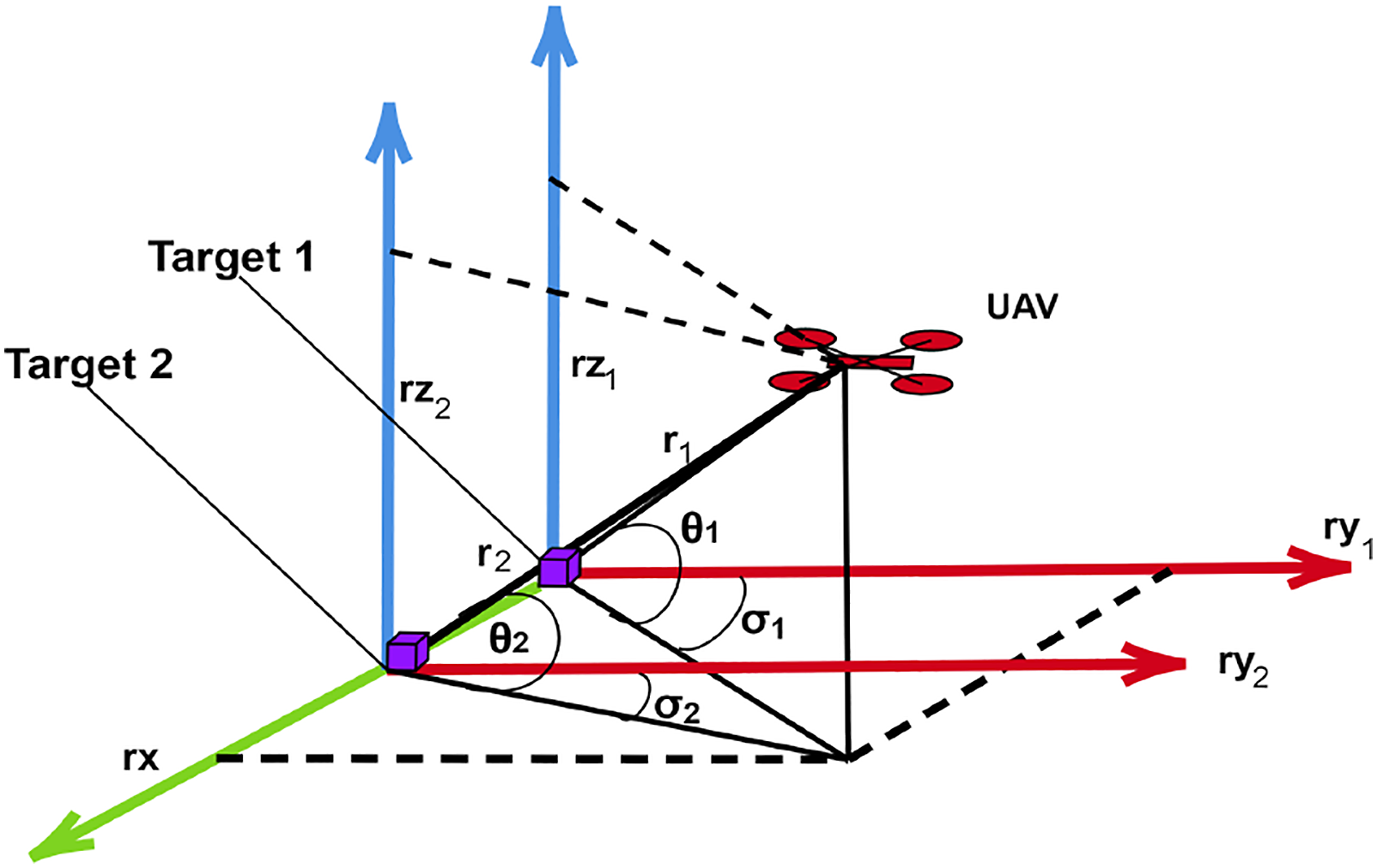
From Figure 7, we can deduce that Vector representations of UAV’s and targets positions.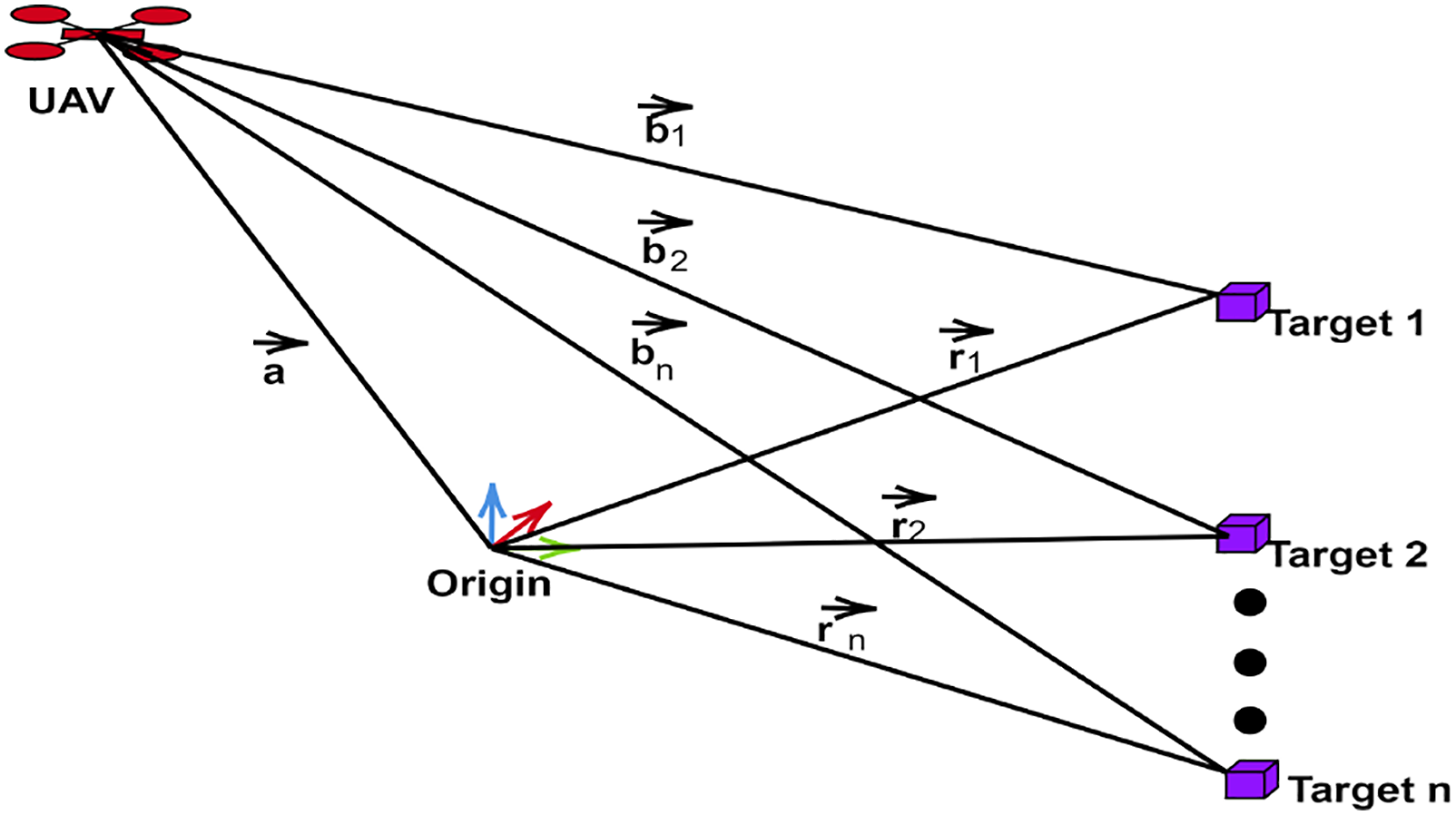
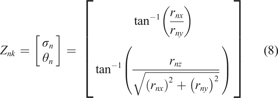
The measurement model is based on the azimuth angle σ and the elevation
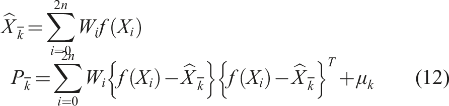
The UKF model constitutes of firstly the time update step then the measurement update step. The time update encompasses the weight and the sigma points calculations. The measurement update utilizes the sigma points to generate covariance matrices and the Kalman gain. 18
The time update
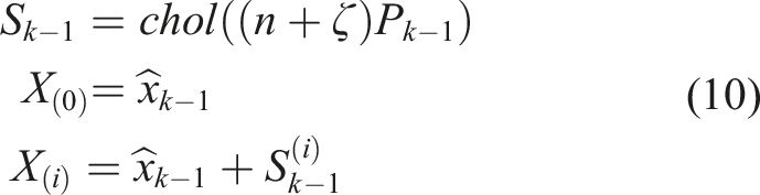
This process includes calculation of the sigma points and their weights and finally obtaining the time update equations after the Cholesky decomposition. We define the weights as
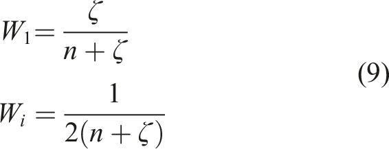
Similarly
Measurement update
The augmented sigma points can be obtained as
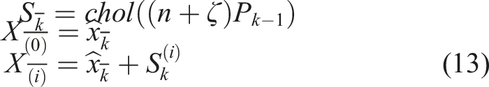
Similarly
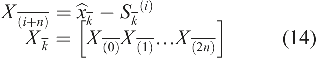
Finally, the measurement covariance and the Kalman gain are calculated as
The final estimated state and it’s covariance are
The position of the targets in ground frame is the output from the estimator.
Gazebo simulation and experimental set-up
Gazebo simulation set-up
For the simulation level verification experiments, the Gazebo environment is used in this paper. A model of the Parrot AR drone was developed in Gazebo,
39
as demonstrated in Figure 8. The drone is equipped with all the sensors (monocular camera, rotors, ultrasonic sensors, etc.) as in the real platform. The properties of the sensors are assigned to match with real characteristics as best as possible. Gazebo environment set-up showing the drone and the targets.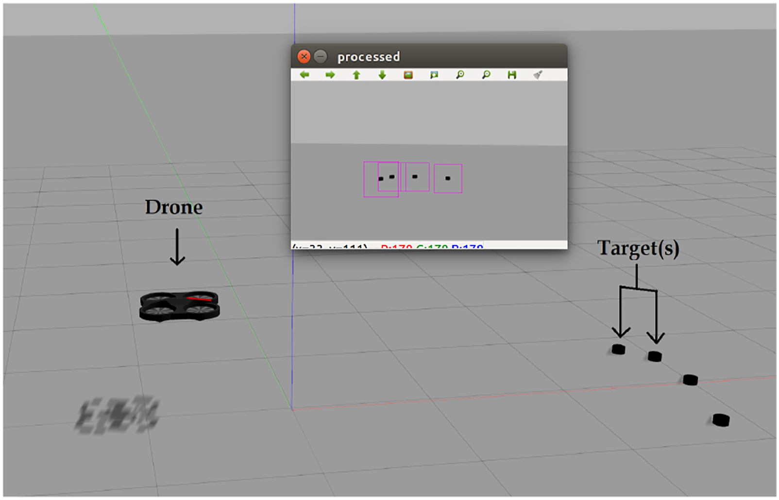
For the simulation works, the ROS is used together with Gazebo. In addition to drone and sensors model, the ROS nodes responsible for the detection and classification of the weed using a DNN, centre pixel extraction on the images, calculating the bearing angles, fusing the bearing angles to estimate world coordinates of the weed with UKF and the trajectory planning and drone driving behave as the same in the real-time. A typical scene in Gazebo is presented in Figure 8. The black dot-like object represents the target/weed.
Experimental set-up
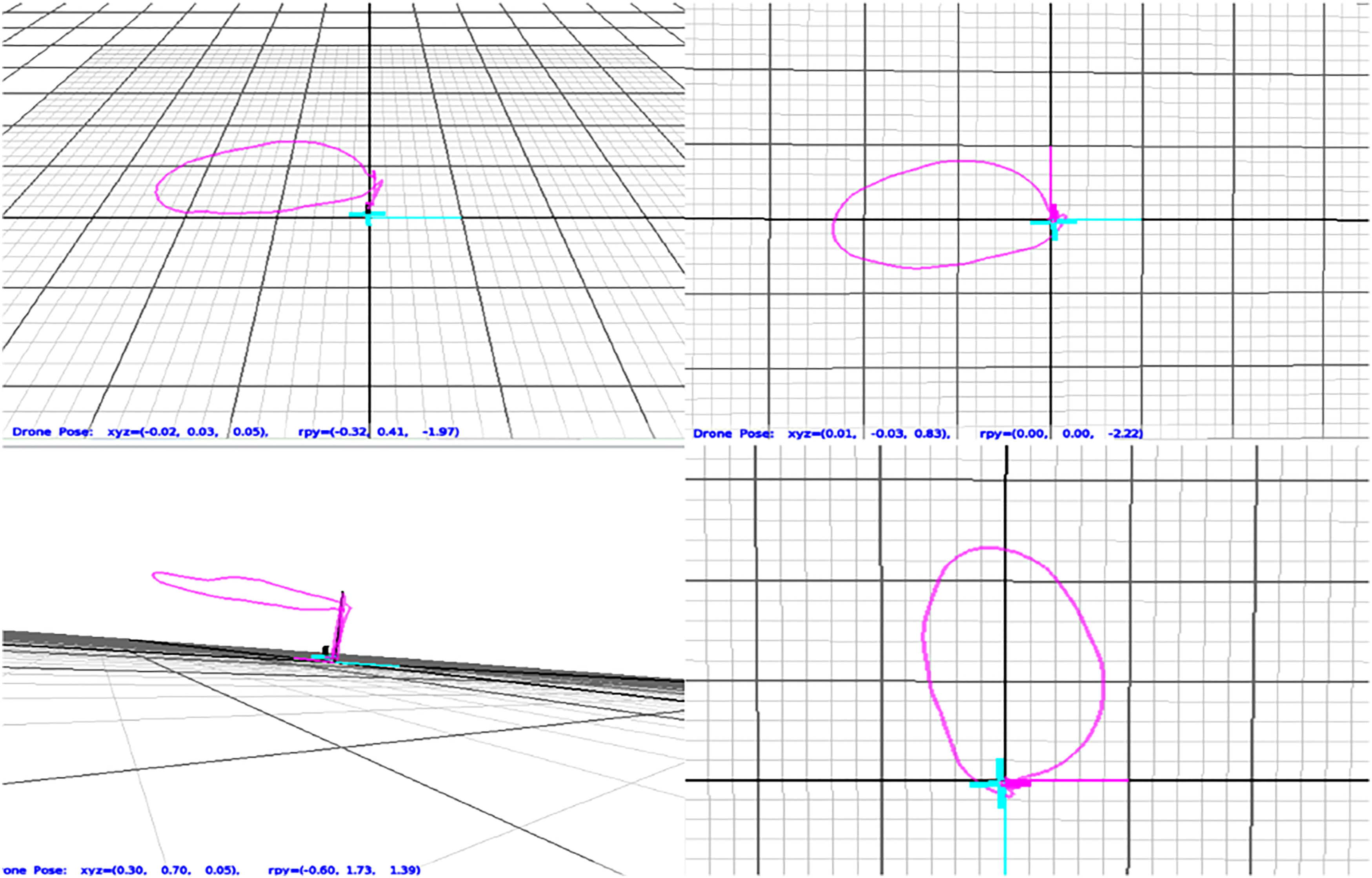
The experimental set-up includes Optitracks tracking system (see Figure 9), the Parrot drone (see Figure 10), the ground station and the target/weed. An indoor scene was created where real weeds were placed at some known positions. The Optitrack system is used to track the drone and also to obtain the ground truth positions of the targets. An actual Parrot drone shown in Figure 10 is subjected to a trajectory while the on-board monocular camera is utilized to detect these weeds. The trajectory parameters are selected such that the targets are covered in the FOV of the drone. A typical trajectory for four targets is seen in Figure 11 using a major axis radius a = 0.6 m and minor axis radius b = 0.4 m with a height of 1 m. Optitrack tracking camera. Parrot AR drone. Obtained trajectory using a major axis radius = 0.6 m and minor axis radius = 0.4 m.
The centre pixels of the detected weeds are processed on the ground station to estimate the relative positions of the weeds. The weights of the fused-YOLO were exported as a static library with a function format which makes it easy to be called from any script. The MKLDNN libraries were linked so that neural network can run on the ground station CPU. 40
It is impossible to connect the workstation to the drone and the Optitracks at the same time. To overcome this issue, the internal configuration of the AR drone is updated so that it serves as a client and can be connected to a local network as shown in Figure 12. Network connection set-up.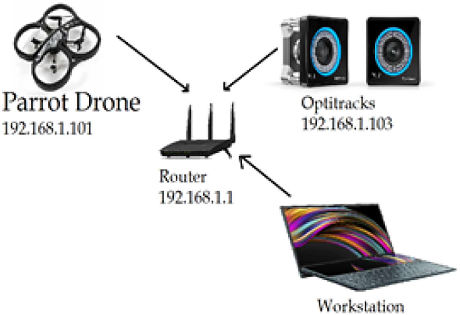
Connecting to the Optitracks is not enough to establish a pipeline to receive position updates, a supporting package is used to receive the broadcasted positions from the Optitracks so it can be used as a ROS topic and can be subscribed by any node. The real-time experiment was carried out on i7 Core CPU. It took approximately 45 seconds to complete the estimation which includes weed detection and localization as well. All the CPU cores were utilized with an average utilization factor of 90% while running the fused-YOLO. The frequency of the CPU was maintained at 2435 MHz.
Results
For both simulation and experimental works, the initialization was done arbitrarily; however, the initial state estimate and its covariance are taken as follows
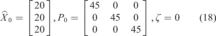
Targets/weeds are placed at different ground truth positions. The drone is placed at [x,y] = [0.00, 0.00]
Simulation results
The simulation results were analyzed by comparing the estimated positions with the ground truth position. Weeds were placed at ground truth positions [x, Coordinate estimation and error (simulation tests along x-axis). The dashed lines represent the ground truth while the continuous lines are the estimations.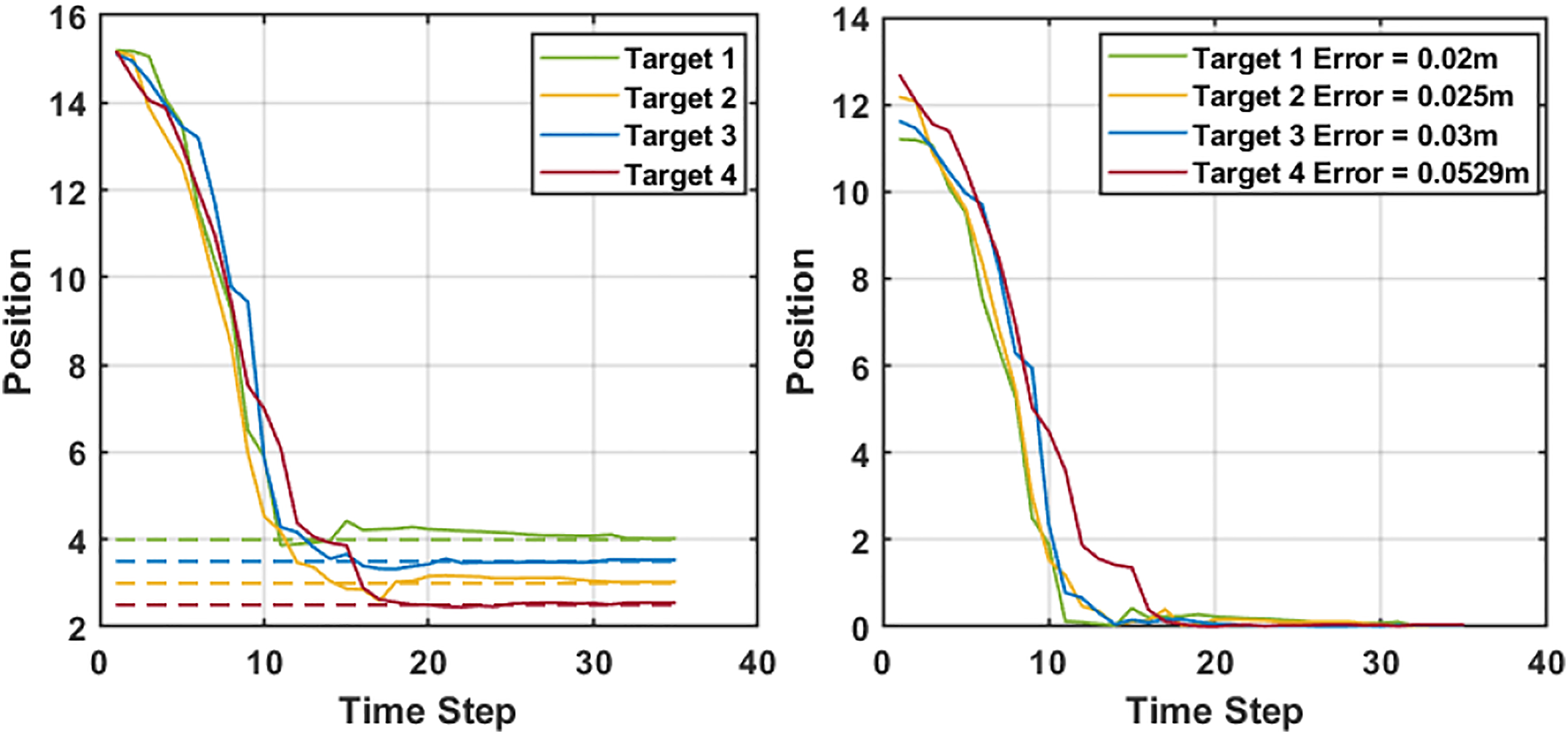
The 2D localization of the weed is performed simultaneously. For the lateral tests, we estimate the y component of the ground truth, that is, [ Coordinate estimation and error (simulation tests along y-axis). The dashed lines represent the ground truth while the continuous lines are the estimations.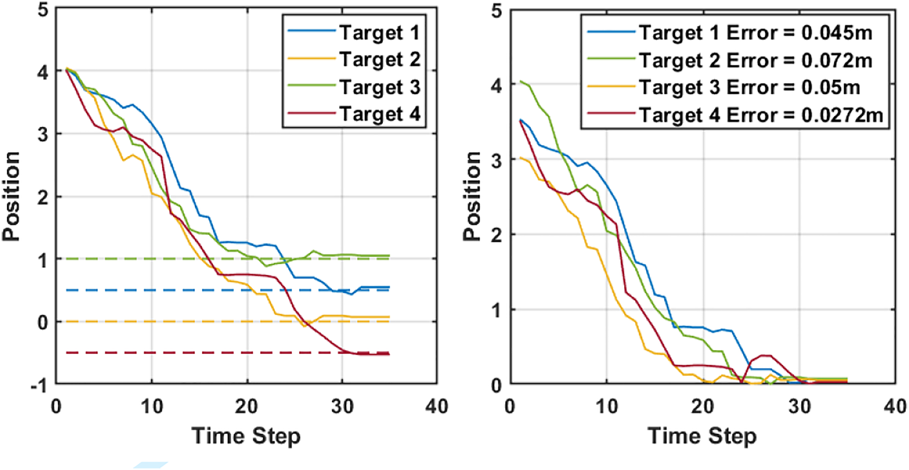
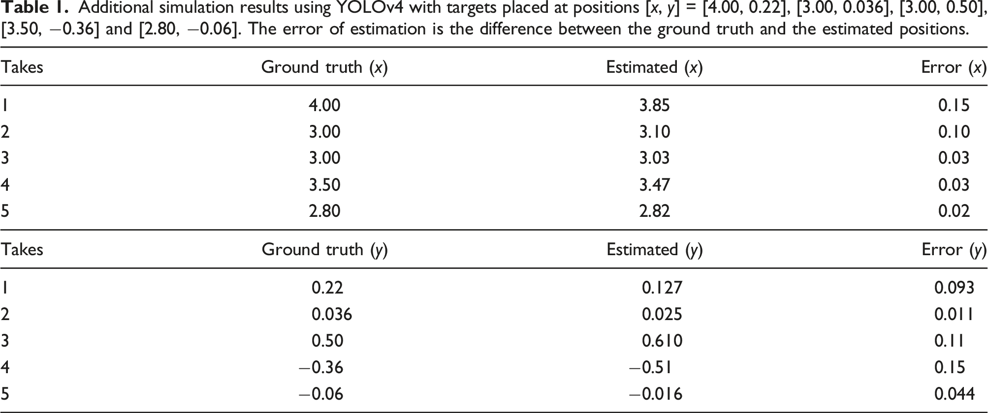
Additional simulation results using YOLOv4 with targets placed at positions [x, y] = [4.00, 0.22], [3.00, 0.036], [3.00, 0.50], [3.50, −0.36] and [2.80, −0.06]. The error of estimation is the difference between the ground truth and the estimated positions.
Experimental results
Detection score
The accuracy of detection has an effect on the overall estimation performance, since the centre of bounding box of the detected weeds is assumed to match the geometric centres of the targets. The detection score evaluates how well a bounding box is assigned to a target Detection score.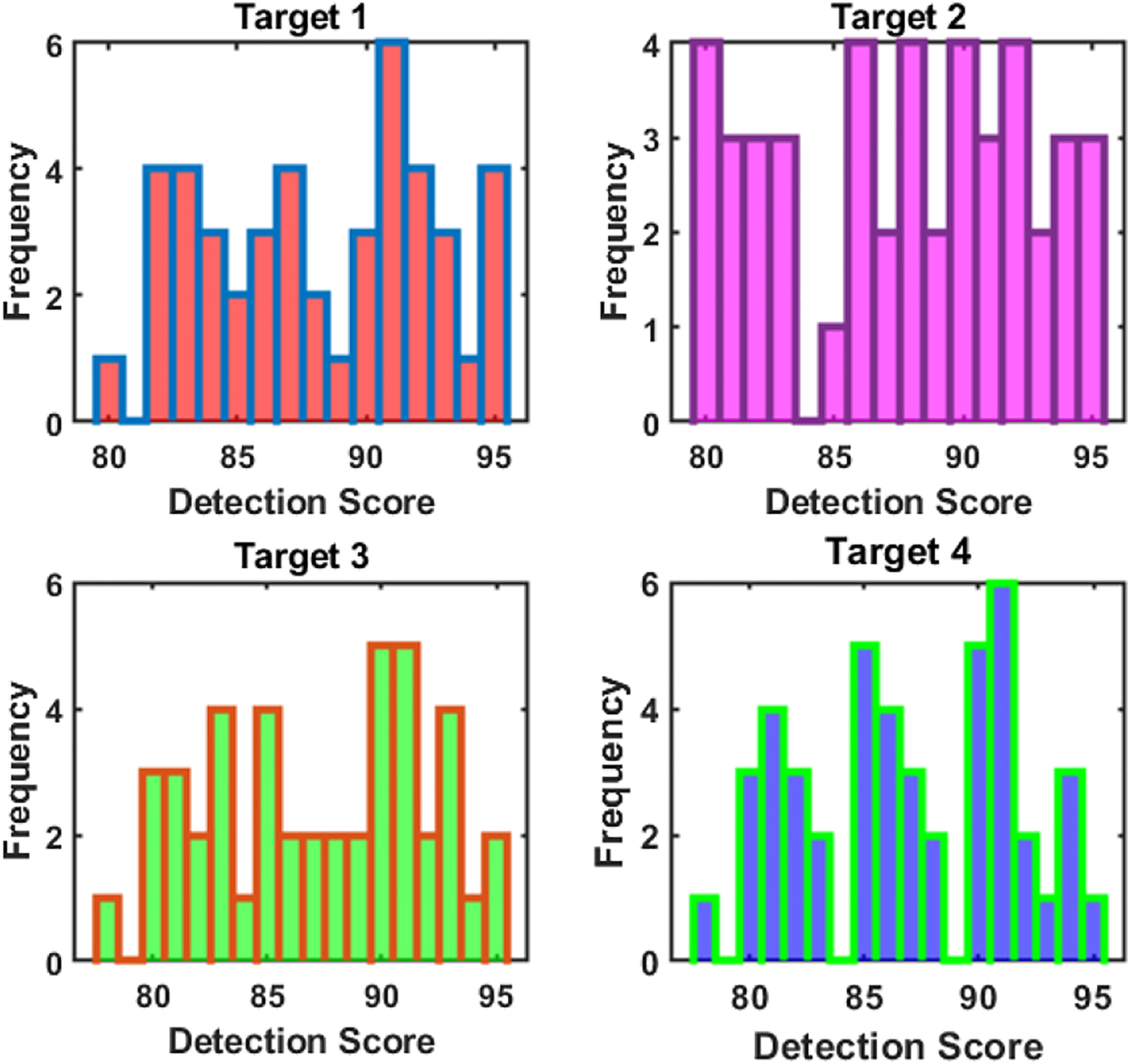
Detection deviation
The detection deviation is defined to indicate how much is the deviation in Detection deviation.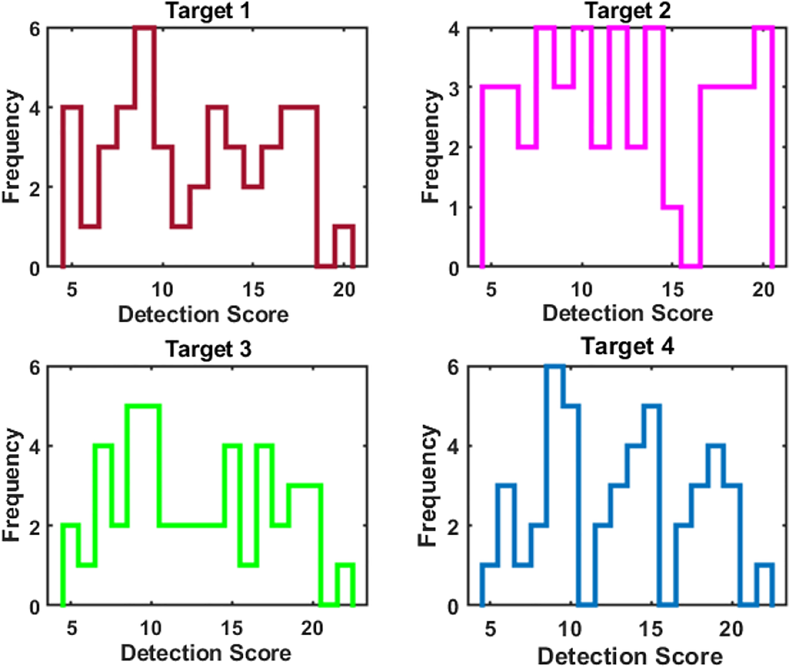
Position estimation
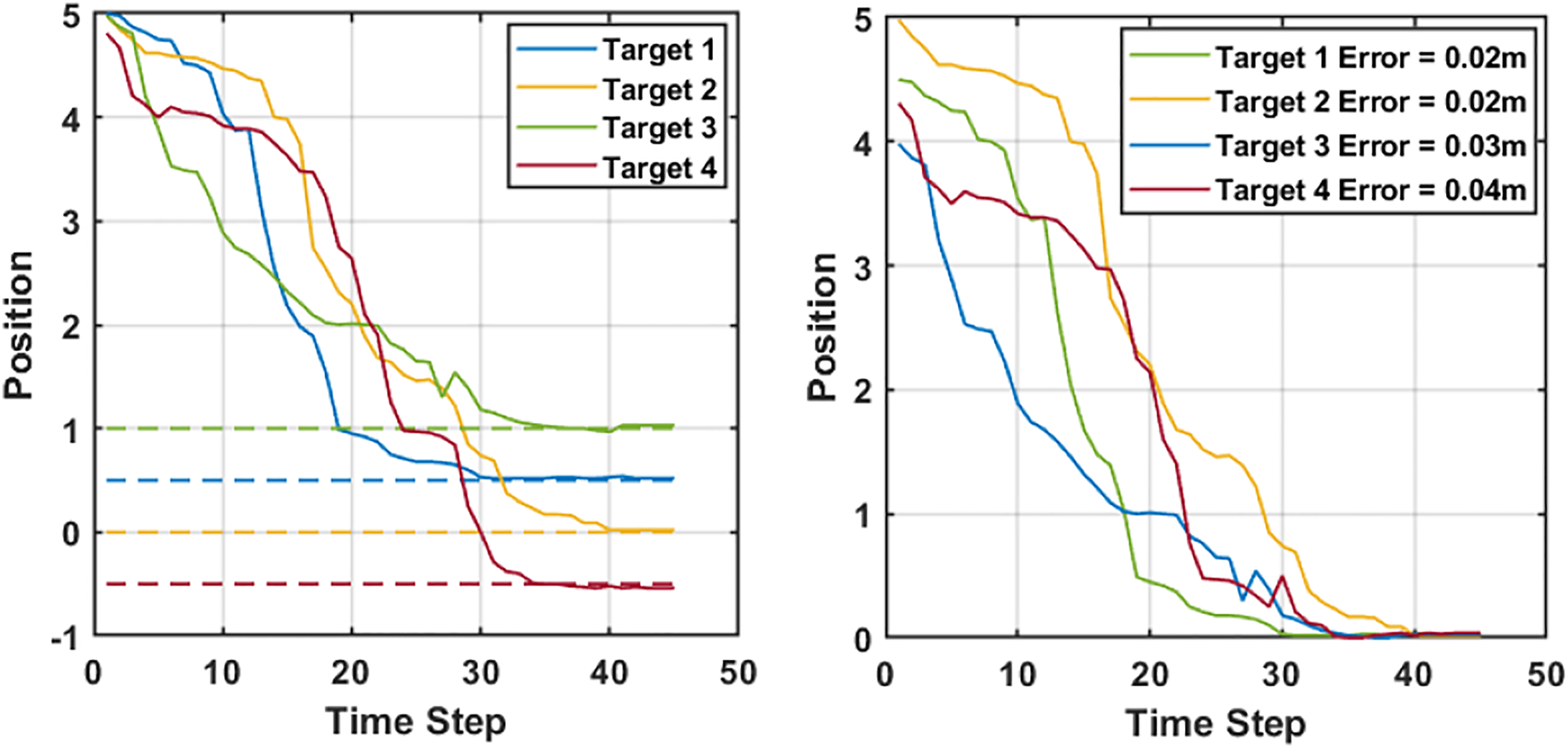
As the drone follows its predefined elliptical trajectory, the depth, the azimuth and elevation angles vary continuously, and the measurements are fused to estimate the positions of targets. Weeds were placed at ground truth positions [x, Coordinate estimation and error (experimental tests along x-axis). The dashed lines represent the ground truth while the continuous lines are the estimations. Coordinate estimation and error (experimental tests along y-axis). The dashed lines represent the ground truth while the continuous lines are the estimations.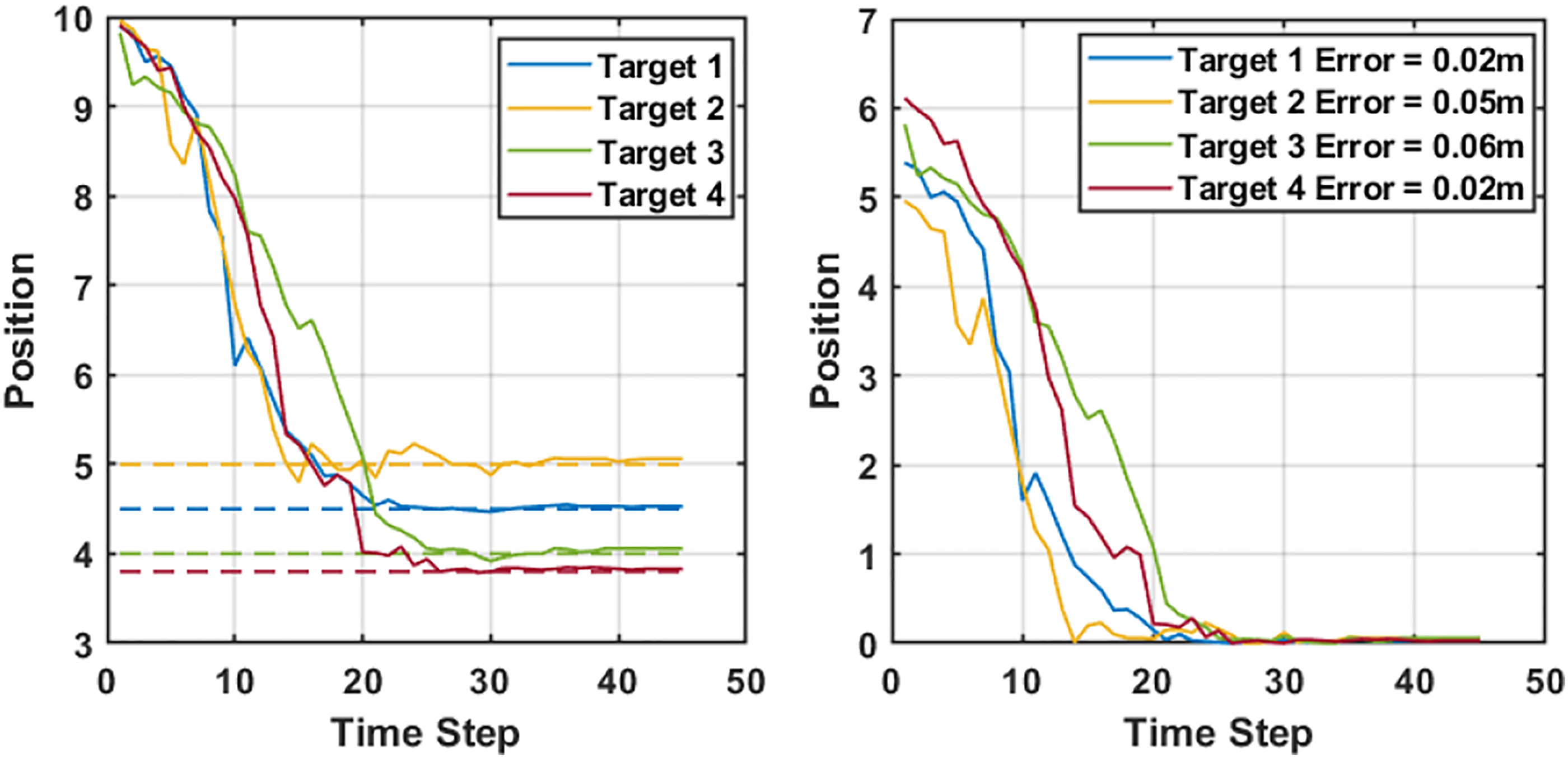
To show the robustness of the proposed scheme, a test is conducted where the Optitrack cannot sufficiently provide feedback to the drone for control. The fixed altitude assumption is violated in these experiments, and consequently, the estimator recorded a greater error in these scenarios, as can be seen in Figure 19. Targets were placed at a y coordinate [ Coordinate estimation and error (experimental tests along y-axis, insufficient Optitrack data case). The dashed lines represent the ground truth while the continuous lines are the estimations.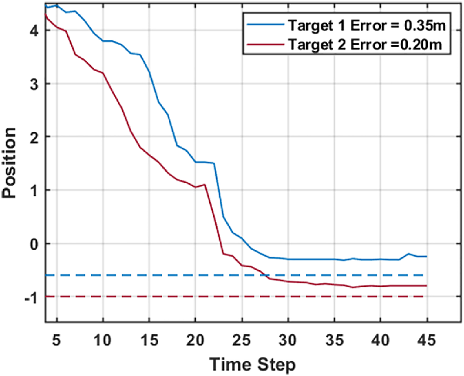
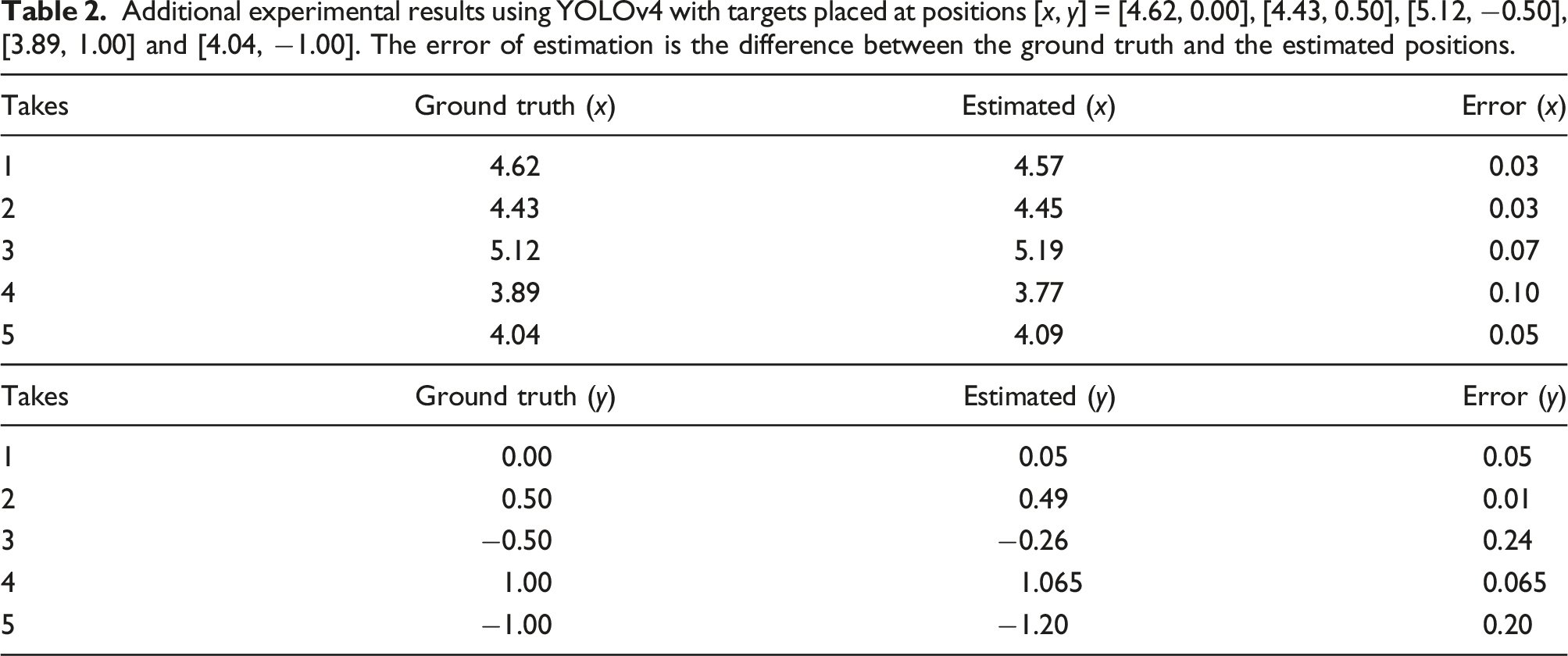
Additional experimental results using YOLOv4 with targets placed at positions [x, y] = [4.62, 0.00], [4.43, 0.50], [5.12, −0.50], [3.89, 1.00] and [4.04, −1.00]. The error of estimation is the difference between the ground truth and the estimated positions.
Depth estimation
The depth, Depth estimation.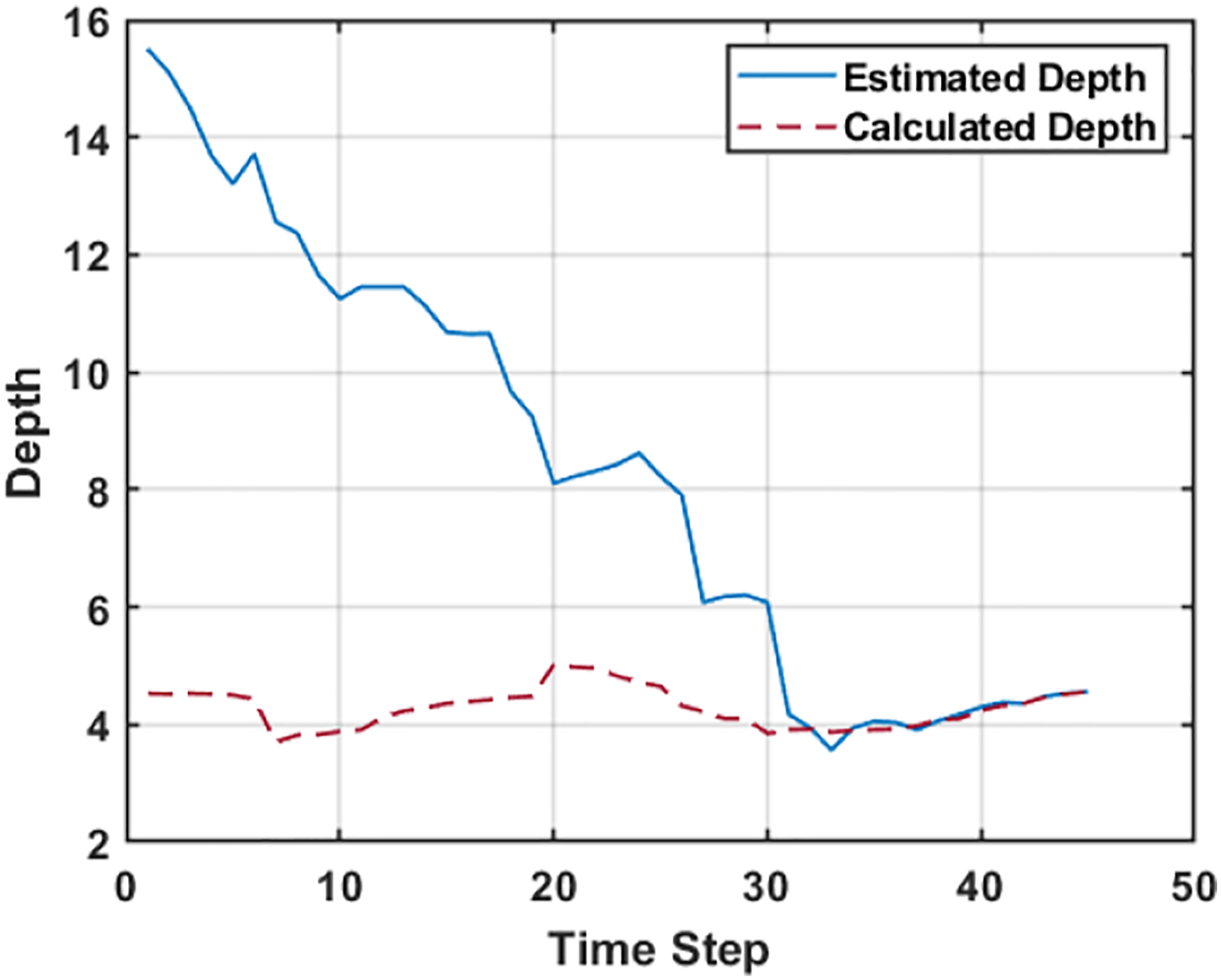
The experimental results converge after 45 seconds while the simulation results converge after 35 seconds. This is majorly due to the latency as the image updates are transported over a network in the experimental set-up. On the other hand, the simulation set-up assumes an ideal world with no update delay.
Detection score comparison
Our pipeline can be utilized with different YOLO versions by simply substituting the detection end of the pipeline. This shows how flexible the pipeline proposed is since it can easily be adapted to other versions of YOLO. This can be done by truncating the final layers of ResNet-50 and utilizing the final activation layer of the RestNet as the feature extraction of the preferred YOLO version as earlier explained in Figure 2. Provided a detection is made and a bounding box is assigned to the target, detected target’s position can be estimated. However, there can be a slight deviation in detection score across different YOLO versions.
Newer versions of YOLO such as YOLOv4 may have better accuracy and FPS. However, these properties may not significantly increase the overall accuracy of the estimation since the detection is performed at regular time steps. Nonetheless, the most sensitive parameter is the detection score which can introduce error to the estimation. A better detection score will result in a better estimation. We define the detection score as how well the centre of the bounding box aligns with the centre pixels of the target. We have compared the detection scores obtained using both YOLOv2
41
and YOLOv4 as the final layers of the proposed architecture across 45 time steps for each target as seen in Figure 21. The overall average detection score (ADS) for the four targets using YOLOv4 is 87.505% while with YOLOv2 it is 86.5%. Although both ADS fall within an acceptable range for this experiment, YOLOv4 is expected to provide a slightly more accurate result than YOLOv2 since it has a better detection score. (a) Detection score comparison between YOLOv2 and YOLOv4 for target 1, (b) detection score comparison between YOLOv2 and YOLOv4 for target 2, (c) detection score comparison between YOLOv2 and YOLOv4 for target 3 and (d) detection score comparison between YOLOv2 and YOLOv4 for target 4.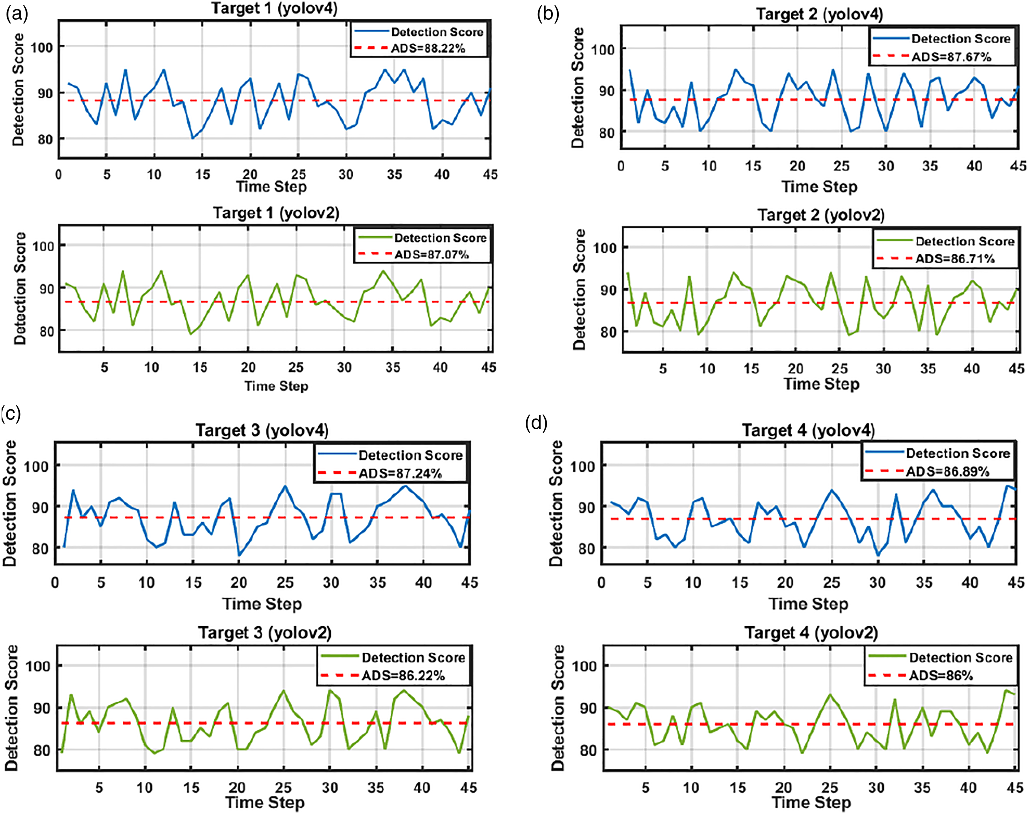
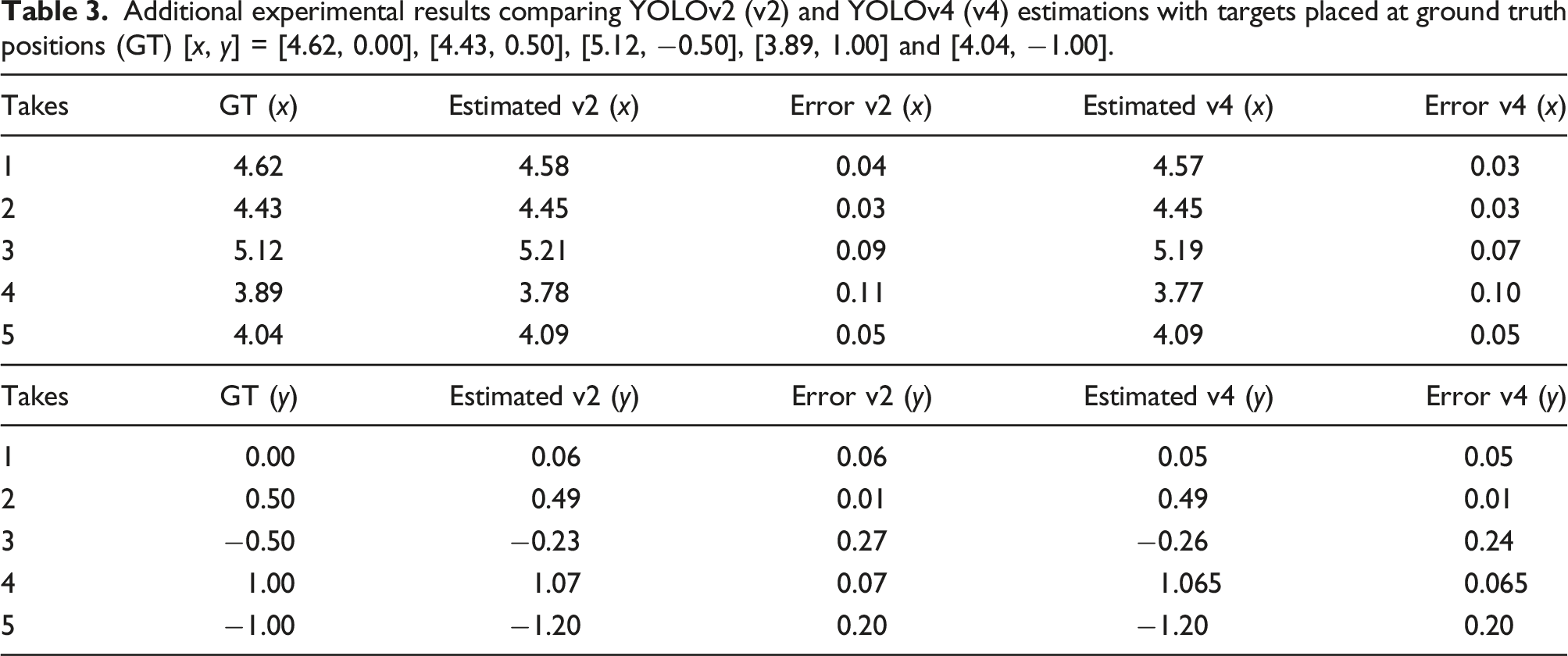
Additional experimental results comparing YOLOv2 (v2) and YOLOv4 (v4) estimations with targets placed at ground truth positions (GT) [x, y] = [4.62, 0.00], [4.43, 0.50], [5.12, −0.50], [3.89, 1.00] and [4.04, −1.00].
Network performance
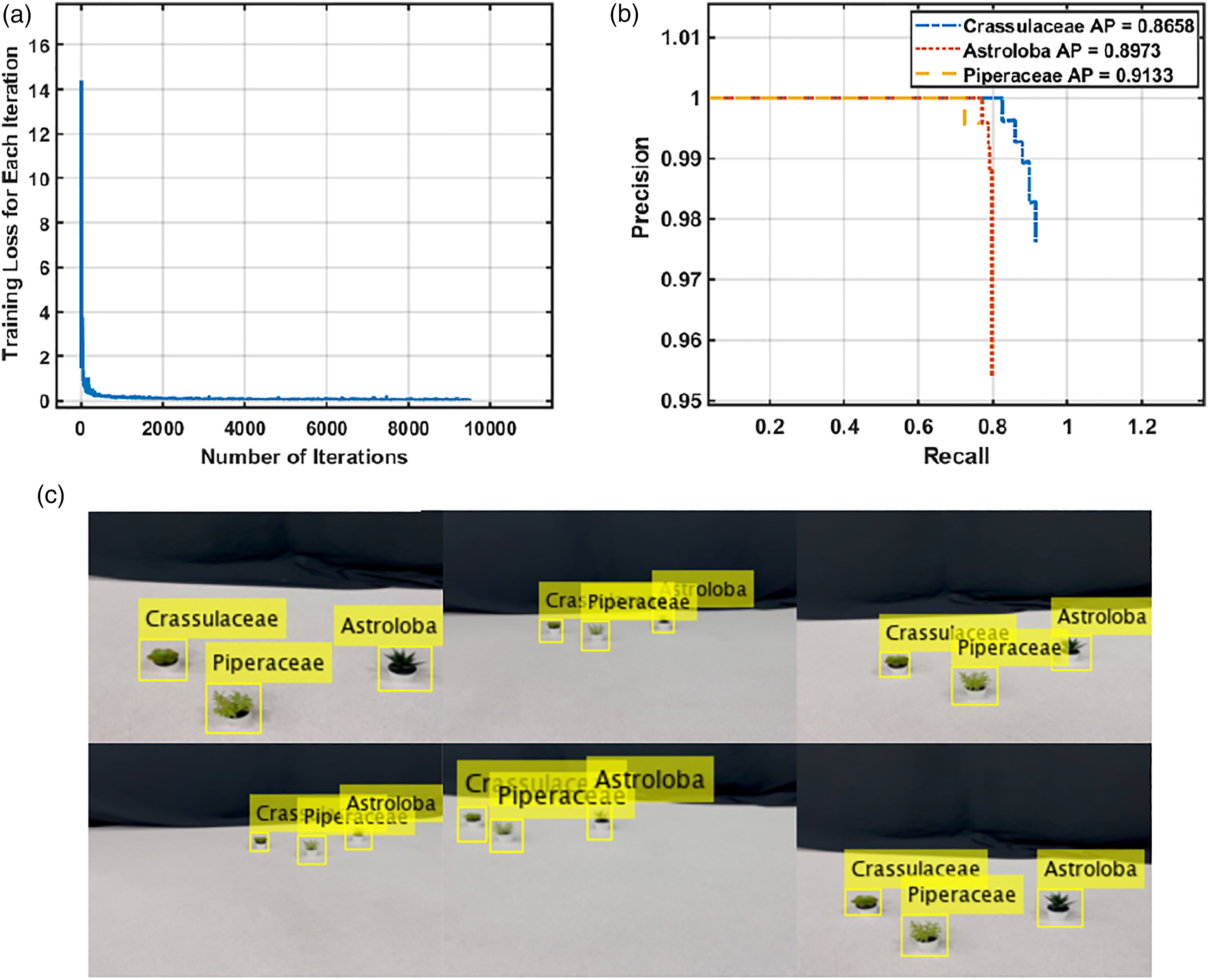
We validated the performance of the proposed network both in the indoor and the outdoor scenarios. Three classes of weeds, namely, Crassulaceae, Astroloba and Piperaceae are used in the experiments. The obtained final training loss was 0.032 for the outdoor training as seen in Figure 22(a). The outdoor validation in Figure 22(b) shows the Average Precision (AP) obtained for these weed classes. Crassulaceae obtained an AP of 0.8643, Astroloba obtained an AP of 0.9362 and Piperaceae obtained an AP of 0.9432 across 443 frames. Samples of the detection using the fused-YOLO network are displayed in Figure 22(c). The bounding boxes as seen in most cases are corresponding to the target’s centre which will facilitate better position estimation. For the indoor setting, a final training loss of 0.0203 was obtained as shown in Figure 23(a). The validation results from Figure 23(b) show the AP of Crassulaceae class at 0.8658, Astroloba at 0.8973, while Piperaceae obtained an AP of 0.9133 evaluated across 315 frames. t(a) Training loss per iteration for fused-YOLO network in an indoor setting, (b) precision/recall results for Crassulaceae, Astroloba and Piperaceae with their respective AP in an indoor setting and (c) qualitative result samples from fused-YOLO network in an indoor setting. (a) Training loss per iteration for fused-YOLO network in an outdoor setting, (b) precision/recall results for Crassulaceae, Astroloba and Piperaceae with their respective AP in an outdoor setting and (c) qualitative result samples from Fused-YOLO network in an outdoor setting.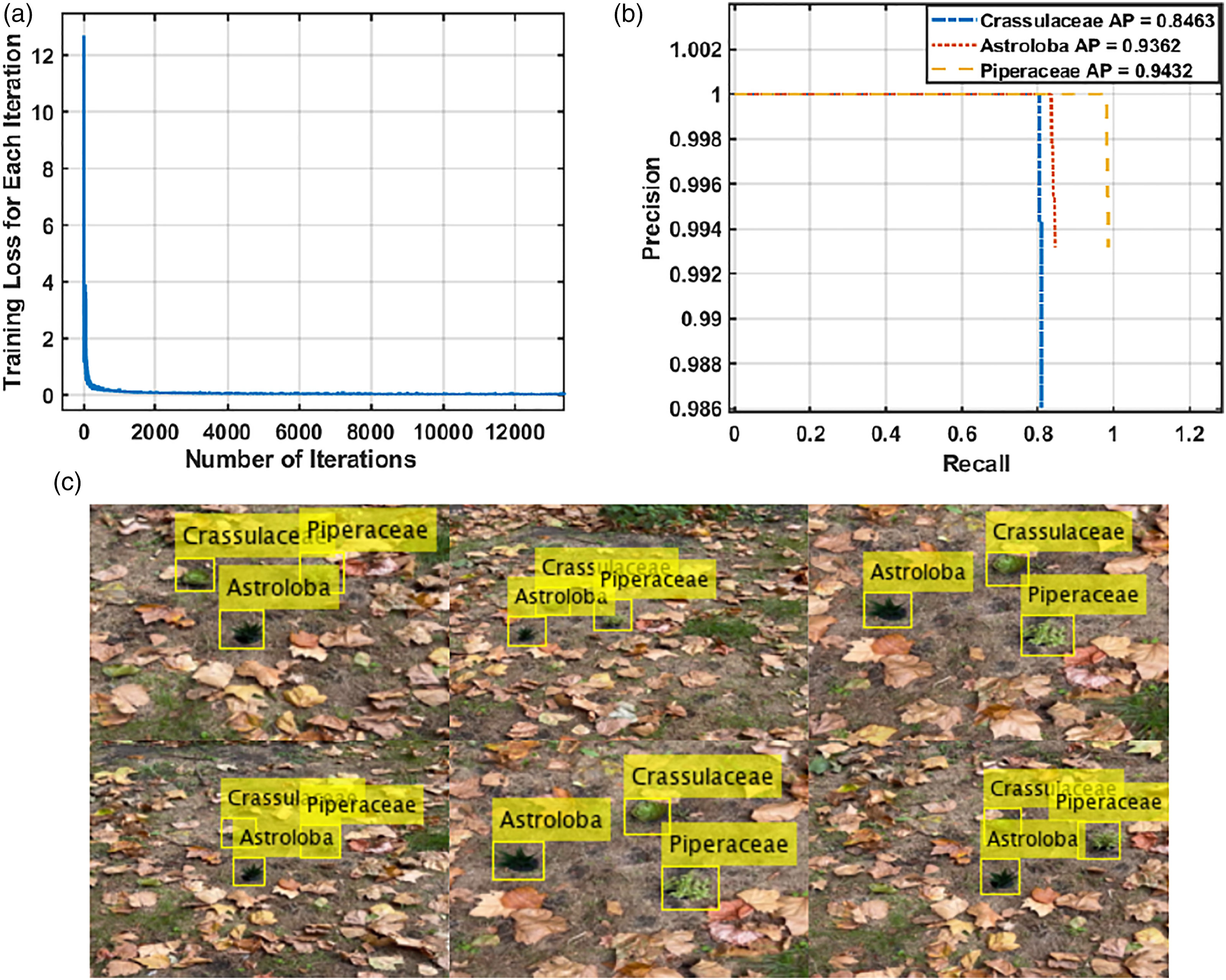
Another experiment was conducted to estimate the positions of the different classes of weeds concurrently. The different classes of weeds (Crassulaceae, Astroloba and Piperaceae) were placed at ground truth positions at [x, Coordinate estimation [x, y] (experimental tests with different classes of weeds). The dashed lines represent the ground truth while the continuous lines are the estimations.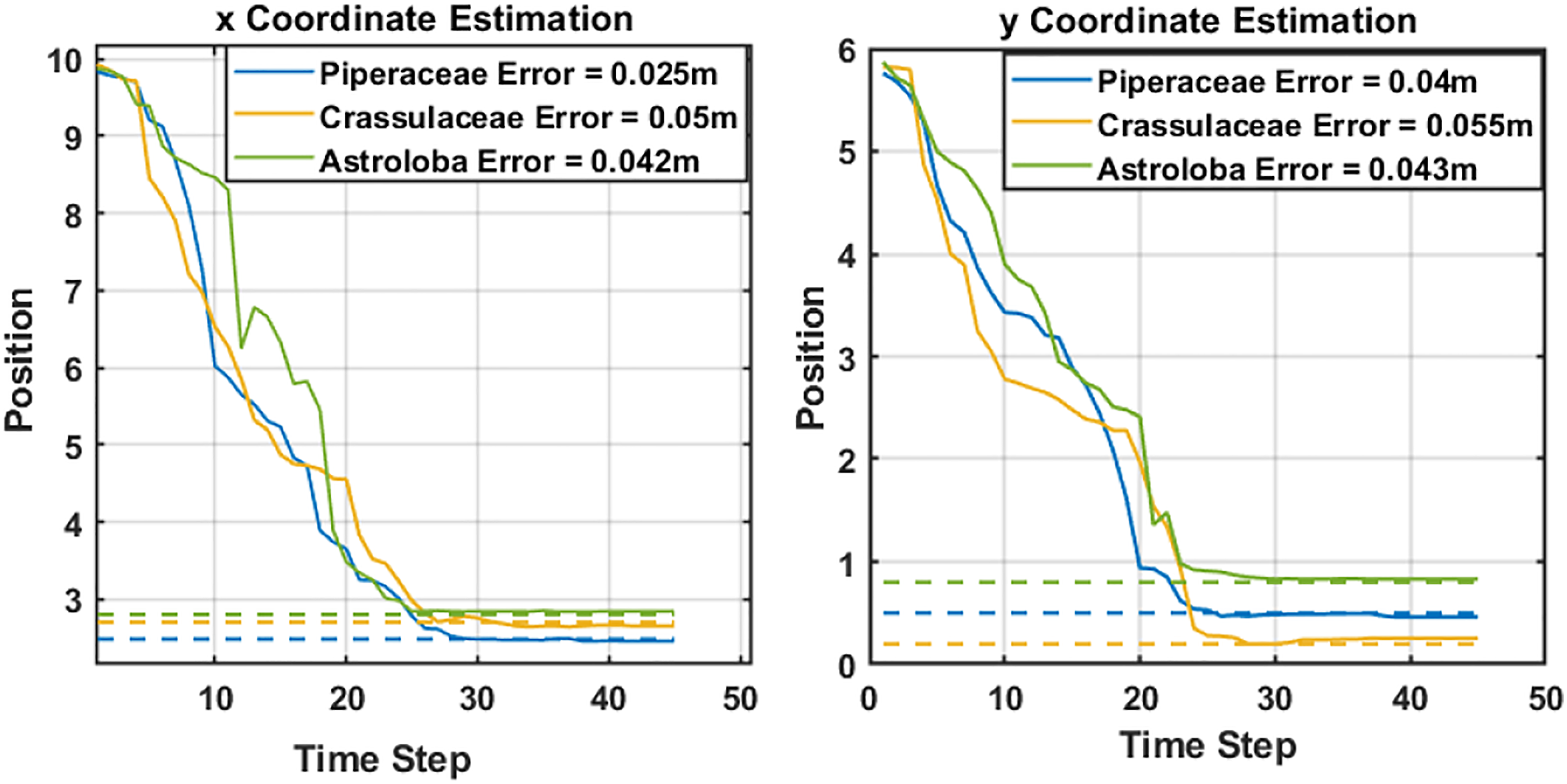
Conclusion
This paper shows the implementation of relative position estimation for multiple targets (weeds) by the combination of UKF with a deep neural network. It addresses the use of sophisticated algorithms for position estimation and detection of weeds, and presented a faster and reliable accuracy using affordable sensors. It extends to not only using bounding boxes for detection but utilizing them for position estimation.
In the proposed solution for weed detection, an affordable UAV platform with a monocular camera is used. Weeds are detected and classified using a trained neural network and the detection boxes are utilized to extract the centre of the target using the image data from the UAV platform which performs a elliptic trajectory and thus forms the basis for the varying bearing angles for UKF estimation. The UKF utilizes the noisy azimuth and elevation angles to perform the estimation.
The simulation results converge after 35 seconds while the experimental results converge after 45 seconds. The detection score was 87.5% in average. Overall average estimator error is (x = 0.056 m, y = 0.0703 m). The proposed method is able to achieve multiple target (weed) position estimation with lesser error margin using an off-the-shelf platform without requiring any sophisticated or additional devices or sensors. The estimation error is measured from the weed’s centre, and most detectable weeds have a cross-section of up to or more than 10 cm. Also, these positions are estimated positions, and mechanical weeding arms or sprayers are usually accompanied with camera to perform visual servoing (post-processing) to fine tune the exact positions of the target, and hence, these results are satisfactory for this mission.
For the future works, this method can be extended to dynamically optimize the trajectory for the estimation for better field of view so more targets/weeds can be estimated. Cooperative estimation can be investigated for faster convergence.
Footnotes
Declaration of conflicting interests
The author(s) declared no potential conflicts of interest with respect to the research, authorship, and/or publication of this article.
Funding
The author(s) received no financial support for the research, authorship, and/or publication of this article.