Sage Journals: Discover world-class research

Abstract

This work addresses a hyperspectral imaging system for maritime surveillance using unmanned aerial vehicles. The objective was to detect the presence of vessels using purely spatial and spectral hyperspectral information. To accomplish this objective, we implemented a novel 3-D convolutional neural network approach and compared against two implementations of other state-of-the-art methods: spectral angle mapper and hyperspectral derivative anomaly detection. The hyperspectral imaging system was developed during the SUNNY project, and the methods were tested using data collected during the project final demonstration, in São Jacinto Air Force Base, Aveiro (Portugal). The obtained results show that a 3-D CNN is able to improve the recall value, depending on the class, by an interval between 27% minimum, to a maximum of over 40%, when compared to spectral angle mapper and hyperspectral derivative anomaly detection approaches. Proving that 3-D CNN deep learning techniques that combine spectral and spatial information can be used to improve the detection of targets classification accuracy in hyperspectral imaging unmanned aerial vehicles maritime surveillance applications.

Keywords

Unmanned aerial vehicle convolutional neural network hyperspectral imaging anomaly detection deep learning

Introduction

The importance of hyperspectral imaging systems for robotic applications is growing. The huge increase in hyperspectral computational systems capacity, together with their dimensions and weight reduction, has encouraged its use in several research and industrial domains such as agriculture,¹ industry,² inspection,³ and surveillance.⁴ The development of novel computational methods, some of them enabling parallel hardware/software implementations, made hyperspectral imaging systems more affordable in terms of price and computational cost, by increasing their capacity to acquire and process huge amounts of data.

One of the most recent applications is the use of hyperspectral imaging systems for maritime surveillance.⁵ This work was performed under the scope of the SUNNY project,⁶ whose objective was to patrol maritime borders using unmanned aerial vehicles (UAVs). For the hyperspectral image sensor, the intended objective was to perform the data processing system onboard the UAV, to acquire hyperspectral imaging data related to the vessels, and to perform vessel detection using solely spatial and spectral information. The information is then transmitted to a Ground Control Station for further processing.

This application imposes two important challenges in the context of Unmanned Aerial Systems: first, the need to customize a hyperspectral payload that holds a sensor unit, a data acquisition unit, and a navigation unit GPS/IMU, which are considerable both in size and weight to fit into an UAV; second and most importantly the development of the capability to detect vessels with hyperspectral image information.

In this article, we will focus our attention on the development of deep learning methods that allow to detect vessels using hyperspectral imaging information. Lots of research efforts have been conducted to use deep learning based approaches for hyperspectral image classification.^{7

–14} However, all of these methods fail in two keypoints:

Almost none correlate spatial and spectral information in the context of hyperspectral images, and the few that do, use it with small-scale networks with relatively fewer number of layers and nodes, instead of a deeper and wider network, leading to poor results.

To overcome the lack of training of hyperspectral imaging data, but also its high dimensionality, most of the state-of-the-art approaches use techniques such as Principal Component Analysis,¹⁵ to work with reduced spectral data inputs. However, these techniques can lead to significant loss of spectral information and do not explore the high-level data dimensionality, leading to an incorrectly exploit of the underlying nonlinear spectral and spatial information.

To overcome such constraints, we implemented a Convolutional Neural Network (CNN) approach for performing maritime target detection that combines hyperspectral spatial and spectral data information. The data used to obtain the results were collected during the final demonstration of the SUNNY project in São Jacinto Air Force Base in Aveiro (Portugal), where a rotary wing UAV equipped with a hyperspectral payload was used to simulate a maritime drug smuggling scenario. The UAV performed multiple flight passages over the vessels that were in the area. To compare the results obtained using the deep learning (CNN) approach, we also implemented our own versions of the Spectral Angle Mapper (SAM) method, which is one of the most used method for anomaly detection using hyperspectral data. We also tested our previous detection method that used an unsupervised approach hyperspectral derivative anomaly detection (HYDADE).

All the aforementioned methods were tested using the same data sets to analyze their capabilities in the detection of vessels in maritime surveillance environment. The results were classified using three different metrics: precision, recall, and F1 score. The results show that the 3-D CNN architecture obtains the best results, being able to increase the recall value by approximately 30%, when compared to the non deep learning approaches. Furthermore, when comparing 3-D CNN results with the SAM and HYDADE results, is possible to observe the lower number of false positives that this approach obtains, proved by the recall and precision numbers that are quite similar when compared with SAM and HYDADE.

The remaining article is structured in the following way: the next section presents related work to the use of deep learning approaches in hyperspectral image classification applications. Afterward, the UAV hyperspectral system setup is described, followed by the methods’ implementation details and obtained results. Finally, some conclusions about the obtained results are drawn, together with some insights on future work directions.

Related work

There are multiple approaches to the deep learning problem, such as AutoEncoders (AE) and Stacked AE,⁷ Deep Belief Networks¹⁶ and CNN.^8,17,18 Recently, CNN have attracted a lot of attention due to their performance in many applications: face recognition,^19,20 object detection,²¹ and video classification.²² CNN is used for hyperspectral data classification due to the ability to automatically learn feature representations through several convolutional blocks, with promising results in terms of accuracy.^23
–25

The CNN hyperspectral image classification approaches can be divided according to their data inputs, namely as follows:

If the method only uses spectral information as presented by Li et al.,²⁶ it is possible to use a 1-D CNN. In this case, the spectral feature of the original image data is used as an input vector, and the 1-D CNN receives $N \times 1$ input vectors (N is the number of spectral bands).^10,27
–29

Another approach is using only spatial information. This type of models considers the neighboring pixels of a certain pixel in the original input image to extract the spatial feature representation. This results in a 2-D CNN, where the input data is a patch of $P \times P$ neighboring pixels, only in the XY space (spatial domain).¹⁰

Another approach is a hybrid approach that considers both types of data (spectral and spatial), where it is possible to combine more information and improve the classification accuracy. This architecture is known as 3-D CNN, and the input data is a patch with all spectral data associated ( $P \times P \times N$ , where P is the patch size, which defines the width and height in the spatial domain, and N is the number of spectral bands) as presented by Chen et al.¹⁰

One example of the CNN use for hyperspectral data classification is given by Chen et al.,¹⁰ where the authors use multiple convolutional layers to extract the nonlinear and invariant deep features, in the spectral–spatial domain, using well-known hyperspectral data sets.^30,31,32 They also investigated some strategies to avoid overfitting during the training of the model. Another example of spectral–spatial feature classification using deep learning is given by Zhao and Du,⁹ where the authors use a CNN to automatically find spatial-related features at higher hierarchical levels. The authors also employ a dimension reduction method before the deep CNN application. Yue et al.³³ show a similar work, where a specific deep CNN is used to learn spectral and spatial features. Hu et al.⁸ only use spectral information to build a CNN able to perform material classification. The work presented by Parkhi et al.¹⁹ shows an application where a CNN based on spectral information is used to automatically extract the hierarchical spectral features and then a 2-D CNN is used to extract the hierarchical space-related features. To combine both information, they use a softmax regression classifier, which allows predicting classification results, and a data augmentation scheme is also used to overcome the problem of hyperspectral limited available training samples.

A more recent approach is performed by Gao et al.,³⁴ where a CNN architecture benefits from the multiple inputs corresponding to various image features, in addition to the concurrent exploitation of both spectral and spatial contextual information. This allows creating a robust and efficient network even with a small number of training samples available. Paoletti et al.²⁴ developed a deep 3-D CNN architecture for spatial–spectral classification of hyperspectral data and also compared all the results obtained with other 1-D, 2-D, and 3-D CNNs already implemented.

Table 1 presents a summary of the related work using CNN method to classify hyperspectral data.

Table 1.

Hyperspectral related work with deep learning summary.

Paper	Method	Application	Data set
Hu et al.⁸	1-D CNN	HSI Classification	Salinas
Lee et al.¹⁷	1-D CNN	HSI Classification	Indian Pines, Salinas, Pavia University
Zhang et al.¹⁸	3-D CNN	HSI Classification	Indian Pines, Botswana, Pavia University
Yu et al.²³	3-D CNN	HSI Classification	Indian Pines, Salinas, Pavia University
Paoletti et al.²⁴	3-D CNN	HSI Classification	Indian Pines, Pavia University
Liu et al.²⁵	Extract features from spectral and spatial domains with two different CNN, and then combine all information into one CNN	HSI Classification	HYDICE HSI
Chen et al.¹⁰	1-D CNN, 2-D CNN and 3-D CNN	HSI Classification	Indian Pines, Pavia University, KSC

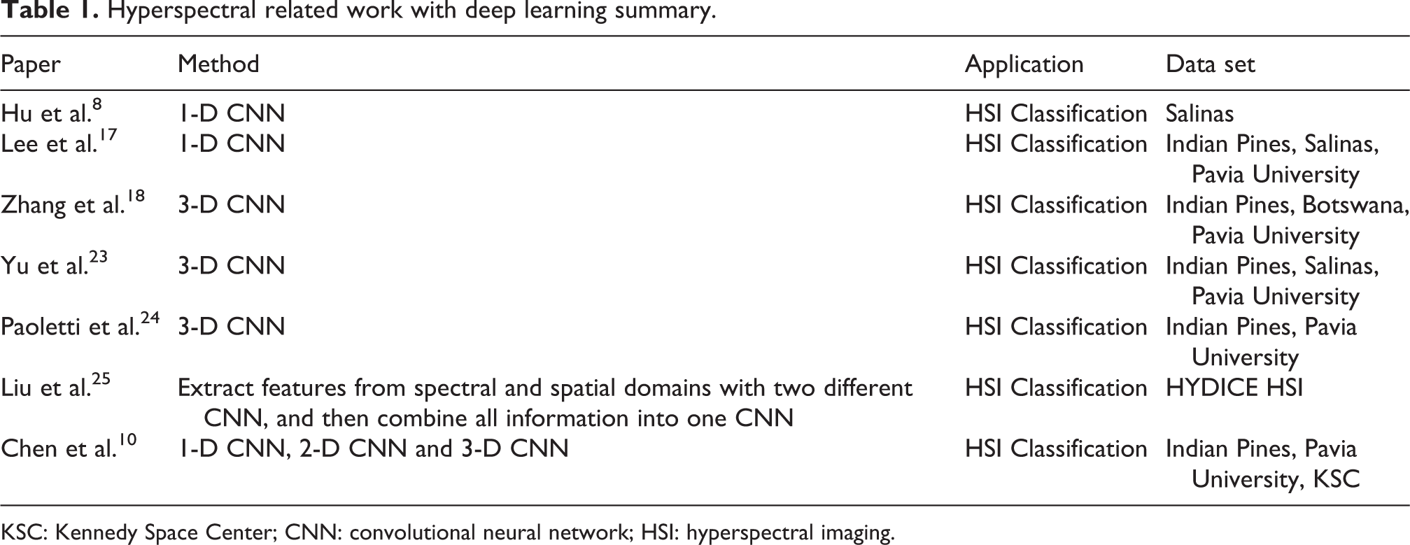
KSC: Kennedy Space Center; CNN: convolutional neural network; HSI: hyperspectral imaging.

Hyperspectral payload UAV integration and data collection

We start this section with a brief introduction and explanation of the hyperspectral payload integration onto the UAV and detail how the hyperspectral data were acquired during the flight trials.

Hyperspectral cameras

Hyperspectral imaging sensors have fine spectral resolution at given wavelengths of illumination, allowing the measurement of the radiation reflected by each pixel in a large number of wavelengths (bands) in the visible and infrared spectrum. To do this, the hyperspectral imaging system uses a spectrometer. This instrument divides the radiation into a number of finite bands and measure the energy in each band. Based on the spectrometer design, the bands may be contiguous or not, with equal width.

Hyperspectral cameras are a combination of spectroscopy and image forming that during the data acquisition create an electromagnetic profile by capturing the intensity of radiation emitted from each pixel at various wavelengths. The collected information is usually combined into a hyperspectral image data cube, which has two spatial dimensions and one spectral dimension. Each pixel (in spatial dimension XY) is a spectrum over the different wavelengths observed by the camera. Figure 1 shows an example of a hyperspectral cube.

Figure 1.

Hyperspectral cube.⁵

The hyperspectral camera utilized in our UAV system payload is a pushbroom hyperspectral camera. Pushbroom cameras acquire data line by line, allowing a full spectral data acquisition simultaneously with spatial line scanning over time, which makes this camera capable of acquiring all the spectral information at the same time. Figure 2 shows an example of a data acquisition method for pushbroom hyperspectral cameras.

Figure 2.

Hyperspectral pushbroom scan.⁵

The hyperspectral system setup displayed in Figure 3 was composed by two subsystems: the hyperspectral imaging system and data processing system. The hyperspectral imaging system used was the SPECIM (Spectral Imaging Ltd., Finland) Aisa Kestrel 16 and is constituted by:

Hyperspectral camera, composed by the sensor, spectrometer, and lens. The data is collected by Camera Link interface and allow the use of an external trigger to control the acquisition. This interface also guarantees sufficient transfer capacity even at the maximum data rates from the camera.

Hyperspectral PC and Control Electronics, composed by a computer motherboard (CPU) with Windows 7, SSD, framelink express frame grabber that allows the connection between the sensor and the CPU for data acquisition, a hyperspectral control board for synchronization between image data and GNSS/IMU data acquisition with 0.1 ms accuracy and hyperspectral camera shutter control, and also a power regulator.

GPS/inertial measurement unit (IMU) unit, with a GPS receiver and an inertial system. This is physically coupled to the camera.

Figure 3.

ETHERAS UAV payload connections. UAV: unmanned aerial vehicle.

The SPECIM Aisa Kestrel 16 characteristics are presented in Table 2.

Table 2.

SPECIM Aisa kestrel 16 characteristics.

Parameter	Kestrel 16
Spectral range	600–1650 nm
Spectral sampling	4 nm
F/#	F2.4
Smile/keystone	<0.15 pixels
Polarization sensitivity	<±2%
SNR (peak)	800
Spatial resolution	320 or 640 pixels
Integration time	Adjustable within frame period
FOV	21.7° or 40°
Electromechanical shutter	Yes
Data interface	Cameralink 14-bit

The data processing system is composed by:

data processing CPU, using Linux Ubuntu 16.04, responsible for the image data acquisition and processing;

eletro-optical camera (EO), a Point Grey Blackfly 3.2 MP Color GigE PoE (Sony IMX265, FLIR Integrated Imaging Solutions Inc., Canada) model, used for confirmations purposes only.

The communication between the hyperspectral CPU and the data processing CPU was accomplished via Ethernet and Serial Port. The Ethernet Port was used to send the image and navigation data, while the Serial Port received the PPS synchronization pulse to synchronize both boards with a common timestamp given by the navigation sensor.

The experimental setup was installed into a rotary wing UAV from a Greek company, ALTUS LSA, named ETHERAS, shown in Figure 4. In Table 3, it is possible to observe some of the UAV characteristics.

Figure 4.

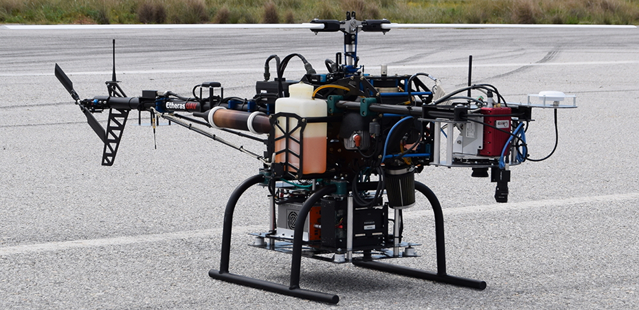
ETHERAS UAV. UAV: unmanned aerial vehicle.

Table 3.

ETHERAS UAV characteristics.

ETHERAS UAV
Gross weight	35 kg
Payload capacity	12 kg
Endurance	60 min
Speed	90 km/h
Range	50 km
Length	1.78 m
Width	18.4 cm

UAV: unmanned aerial vehicle.

The payload was installed in two major different areas of the UAV: the bottom tray hold all computational power equipment, while the other sensor parts (cameras and inertial system) were placed in the front part of the UAV, to diminish the occlusions and electromagnetic interference.

Spectrum processing

To process the hyperspectral data, first we need to preprocess the raw hyperspectral data. This preprocessing is composed by two main procedures: the reference pattern and the conversion of the raw sensor data into radiance at-sensor values.

The first, reference pattern, is established by analyzing and subtracting to the acquired data the average of the dark frames value, where the dark frames are images taken with the camera shutter closed. To accomplish the conversion from the raw sensor data into radiance at-sensor values, it is necessary to use the equation (1)

L_{λ} = Gain \times Pixel Value + Offset

where the λ refers to the wavelength. The gain is a fixed value per pixel and wavelength given by a calibration performed by the manufacturer, while the offset is set to zero.

Target detection methods

Hyperspectral image sensors are advanced devices capable to return a considerable amount of information about a scene in just one frame. Given this information, we need to process the collected data to provide usable surveillance information using target detection methods.

For the purpose of this work, we implemented three different methods to detect and identify vessels. The first was a CNN, a supervised method, with a 3-D approach that allows to use both spatial and spectral information given by the hyperspectral camera. The second method tested was SAM,³⁵ a supervised method that uses the angle between spectra to identify their similarity and finally HYDADE,⁵ our previous anomaly detection method.

Deep CNN

In this work, we implemented a 3-D deep CNN architecture using both spatial and spectral data information. A complete CNN stage is constituted by a convolutional layer with a nonlinear operation and a pooling layer. Joining multiple convolution layers with a nonlinear operation and several pooling layers is possible to formulate a deep CNN. A typical CNN is composed by 1–3 complete stages followed by one or more fully connected layers and a final classifier layer. The convolutional layer uses a filter defined by the user and then convolve the filter in a small part of the input data. The main goal of this layer is to identify certain features from the previous layer and mapping their appearance to a feature map.³⁶ The resulting output volume of a layer l is a feature map with size $d^{l} \times d^{l} \times k^{l}$ and stores the information where the feature occurs in the original input volume. This output is calculated with equation (2), where $i \in [1, k^{l}]$ , $B^{l}$ is the bias matrix of the layer l, and $W_{i j}^{l}$ is the kernel that connects the jth feature map in layer $l - 1 (z_{j}^{l - 1})$ with the ith feature map in layer l

z_{i}^{l} = B^{l} + \sum_{j = 1}^{k^{l - 1}} W_{i j}^{l} \times z_{j}^{l - 1}

The nonlinearity layer embeds a nonlinear function (such as Rectified Linear Unit (ReLU),^37
–39 which is applied to each feature map component to learn nonlinear representations. The pooling layer makes the features invariant from the location and summarizes the output of multiple neurons in convolutional layers using a pooling function. In the CNN method, this is a max polling layer and allows to reduce the spatial size of the output.

Our approach also holds dropout layers to prevent overfitting. The dropout layer deactivates a percentage of neurons during the training stage, improving generalization because each layer will learn the same characteristics with different neurons. These are usually applied after the fully connected layers because of their large parameters number, which increases the overfitting probability of these layers. However, due to the stochastic regularization used in the dropout layers, in practice, these layers can be applied in any place of the network. The dropout probability can be changed according to the desired regularization impact.

To generate enlarged and dense feature maps and to allow the network to increase the resolution of the output map, we implemented deconvolution layers after the convolutional layer, also known as transposed convolution layer. Despite mathematically performing the operations corresponding to the second designation, the final result will be similar to a deconvolution.

The input of the first layer of our CNN implementation is a patch built from the data set, as observed in Figure 5, where the data set hypercube is shown. This hypercube contains all the data used for these tests, and each portion of the data set will be included in a patch. This patch is given as an input to the first CNN layer.

Figure 5.

Data set hypercube and an example of the 3-D patch scheme implemented.

For the hyperspectral data, each pixel of a hyperspectral scan line that is acquired can belong to a different class. Which means that an individual line can hold all the classes present in the data set. However, if only one line is considered, the spatial information is going to be lost. To exploit the rich spectral and spatial information contained in the hyperspectral data, the CNN is fed with a neighborhood window centered around each pixel vector, which means that the input layer accepts a patch with the size $p_{w} \times p_{h} \times n$ , where $p_{w}$ and $p_{h}$ represent the width and height, respectively, defined by the patch value, and n is the number of bands. The label of each patch is given by the label of the central pixel of the patch, located in $[p / 2 + 1, p / 2 + 1, n]$ .

Afterward, the data is divided into 3-D patches and is grouped into batches of size a and sent to the CNN, where the first convolution layer receives the $d \times d \times n$ patches. This layer is composed by $r^{c 1}$ filters of $d^{c 1} \times d^{c 1} \times b^{c 1}$ , where $b^{c 1}$ represents the number of bands, the stride is fixed to 1, and there is no padding, with a ReLU function. This layer is followed by another convolutional layer with the same characteristics, and then the ReLU function is applied and the $r^{c 1}$ feature maps generated by the second convolutional layer are sent to the first MaxPool layer, with a $d^{m p 1} \times d^{m p 1}$ kernel, stride of 2 and no padding. The output with size $l^{m p 1} \times l^{m p 1} \times r^{c 1}$ is sent to the deconvolutional layer with $r^{d c 1}$ filters of size $d^{d c 1} \times d^{d c 1} \times b^{d c 1}$ . This output is sent to the third convolutional layer with $r^{c 3}$ filters of size $d^{c 3} \times d^{c 3} \times b^{c 3}$ , with the stride fixed to 1 and no padding. Again, a ReLU function is applied, and then the $r^{c 3}$ feature maps generated by the third convolutional layer are sent to the second and last MaxPool layer, with the stride equal to 2 and no padding. The output has the size $l^{m p 2} \times l^{m p 2} \times r^{c 3}$ is reshaped and sent to the fully connected layer. In this CNN, there are three fully connected layers, where the first two layers compute their output as $y^{f c} = f (w^{f c} y^{f c - 1} + b^{f c})$ , where $w^{f c}$ are the weight matrices, $b^{f c}$ are the bias vectors, $y^{f c - 1}$ is the output of the previous layer, and the activation function ( $f (\cdot)$ ) is ReLU. The last fully connected layer is a softmax function as $y^{f c 3} = w^{f c 3} y^{f c 3} + b^{f c 3}$ , where $y^{f c 3}$ are the true labels for the input data. After each fully connected layer is applied a dropout layer with a rate of 0.5. The architecture of the CNN is displayed in Figure 6.

Figure 6.

CNN architecture scheme. CNN: convolutional neural network.

The loss function used is a sparse softmax cross entropy, which applies the cross-entropy to determine the loss of the CNN model. The initialization of all weights and bias is done using the Xavier initializer,⁴⁰ which allows the CNN to gain more stability. The Adagrad optimizer⁴¹ is used for learning rate adaptation.

The CNN was implemented using the TensorFlow⁴² open source library for machine learning, optimized for GPU utilization.

Spectral angle mapper

SAM is a supervised method, which compares a reference spectrum with the image spectrum. With this comparison, it is possible to determine the angle between both spectra, denoted as spectral angle. The value of this angle represents the similarity between the spectrum, where the smaller angles represent closer matches to the reference spectrum. In this method, it is usual to implement two different thresholds, one to prevent that pixels further away than a given value are not classified and another to limit the maximum value at which the spectra can be considered as the same class.

The value of the spectral angle is given by

α = {cos}^{- 1} (\frac{\sum_{i = 1}^{n b} t_{i} r_{i}}{\sqrt{\sum_{i = 1}^{n b} t_{i}^{2}} \sqrt{\sum_{i = 1}^{n b} r_{i}^{2}}})

where r represents the reference spectrum, t is the image spectrum, and $n b$ corresponds to the number of bands.

Hyperspectral derivative anomaly detection

HYDADE is an anomaly detection method that analyzes the transitions/existing peaks in the spectrum response. This is done with the processing of the first and second derivative of the acquired spectrum for each pixel. This method uses a two-step procedure to segment the target pixels from the background. In the first phase, it tests if the first derivative of the spectrum is higher than a predetermined threshold (that was found empirically based on the acquired data), and if it is higher than the threshold, it means that the pixel is a good candidate (possible target pixel). This allows a quick separation of the target candidate pixels from the background. The second step consists of a deeper analysis of the candidate pixels. For this, it is necessary to count the number of peaks of the first and second derivative of each candidate pixel. Based on this procedure, it is possible to obtain the spectrum data smoothness and detect transitions in the spectrum and then group the different pixels into clusters based on their similarity information. The number of peaks is compared with an adaptive threshold for each derivative. A more detailed description of this method can be found in the study by Freitas et al.⁵

Results

During this section, we will present the results obtained with the data collected in the scope of the SUNNY project.

Flight experiment

The SUNNY project final demonstration field trials took place in São Jacinto Air Force Base, in Aveiro (Portugal). The data were collected during the 30th of April flight, where two boats of the same material were in the water. The mission objective was to detect the boats using only hyperspectral image information. Figure 7(b) shows the boats during the rehearsal of a drug smuggling scenario.

Figure 7.

Data set collection elements: (a) São Jacinto air force base and (b) boats with an illegal behavior.

The SUNNY demonstration scenario consisted of a 12-m fishing boat approaching the surveillance area, with a speed not higher than 5 knots. Then, an 8-m speedboat leaves the harbor heading to the fishing boat, with a speed not higher than 3 knots. The two boats meet at the open sea and leash each other, as it is possible to observe in Figure 7(b), where the people on the boat exchange possible illegal substances. Finally, the speedboat gets in motion heading to the coastline while the fishing boat changes course as its initial heading. There were two different boats used during the SUNNY project demonstration: a recreational vessel and also a fishing vessel. These are vessels with easy access, which can be easily rented, bought or even stolen for illegal operations. They also allow a considerable amount of payload and due to their physical characteristics (small to medium size, white color) typically do not raise suspicion to maritime authority.

In Figure 8, it is possible to observe the UAV trajectory during the flight and also the boats’ location. The UAV took off from the São Jacinto airfield runway with an interception trajectory toward the boats. The flight altitude of the UAV was 150 m.

Figure 8.

ETHERAS UAV trajectory in white, and the two boats’ locations are represented by the red markers. UAV: unmanned aerial vehicle.

To have an easy comprehension of the results, it is necessary to define the metrics used to evaluate the methods. The results are presented in two distinct shapes: through images, where some key points are showed in the image, and also using three different metrics, precision, recall, and the F1 score, which are usually the metrics for this type of systems.

In the case of the unsupervised method, HYDADE, we consider only two classes: boat or water. In this case, the calculation of the three metrics is performed directly based on the number of true positives and negatives and false positives and negatives. However, in the case of the supervised method, CNN, we consider three classes: boat, light water, and dark water. In this case, we use an approach one against all to calculate precision and recall values and compare the true positives of each class versus the false negatives and positives of the remaining classes. The unsupervised methods used are anomaly detection methods, which means that they detect objects/materials from the background. To detect light water, these methods should be able to detect non-background items and also determine their object class. However, due to the light reflection, the difference between the light water spectrum and some boat pixels spectrum is reduced, which will lead to false positives. In the case of anomaly detection, due to the spectra similarity, it is not possible to make these type of distinction. However, CNN is a supervised method, which will allow to train the method for each class, and consequently allow the distinction between similar spectra. This distinction improves the results as shown in the results section.

First, we present the results of the CNN method, where we considered three different classes: boat, light water, and dark water. This division was created due to the similarity between some light water and boat points, mainly due to the water that rises around the boat during its movement. Then, we present the results for SAM using the same class division. Finally, we present the results obtained for the unsupervised method, HYDADE, in which we consider only two classes: boat and water. In this case, the method only detects anomalies, so the boat is considered an anomaly when compared to the background (water).

To test the CNN method, we implemented the architecture displayed in Figure 6, using a Nvidia Jetson TX2 (NVIDIA, Santa Clara, CA), with 8 GB LPDDR4 RAM and 32 GB eMMC 5.1 Flash Storage, using the TensorFlow open-source library.

For the CNN implementation, it was required to divide the data into training and test data. The training data is used to train the CNN, and then, the trained network is evaluated with the test data. Due to the class imbalance problem,⁴³ because of the quantity of water data when compared with the boat data, only a few samples of each class were selected for the training data. The samples were randomly selected, a standard procedure in a deep learning data set. In this case, 75% of the data set was used for training, while the rest is used for testing, and the number of selected samples was 500 samples per class.

The SAM implementation is similar to CNN implementation, and the data division and the number of samples per class are equal for both cases. For this two methods, the data set was divided into three different classes: light water, dark water, and boat. The batch size was fixed with the value 100, and the learning rate value was 0.005. The maximum step number was 500, while the epoch number was 20. The optimizer used was the Adagrad optimizer, while the patch size was a square with 7 pixels. The data set used is a boat data combination collected in São Jacinto Airfield, with 111 lines, 640 pixels, and 384 bands, and during the course of the flight, the UAV acquired boat data six times.

In Figure 9, it is possible to observe one image constructed with the data set, using single band information.

Figure 9.

Data set image constructed using only one band information.

CNN results

In Figure 10, one can observe the results for the CNN implementation. We start by showing a ground truth image with the classes of each pixel, which is presented in the Figure 11 top left image, where the red points symbolize the boat points, the blue points represent the light water points, and all other pixels without color correspond to dark water.

Figure 10.

CNN results: (a to f) the red points represent the boat points, the blue points represent the light water points and all the points with no color represent the dark water pixels. CNN: convolutional neural network.

Figure 11.

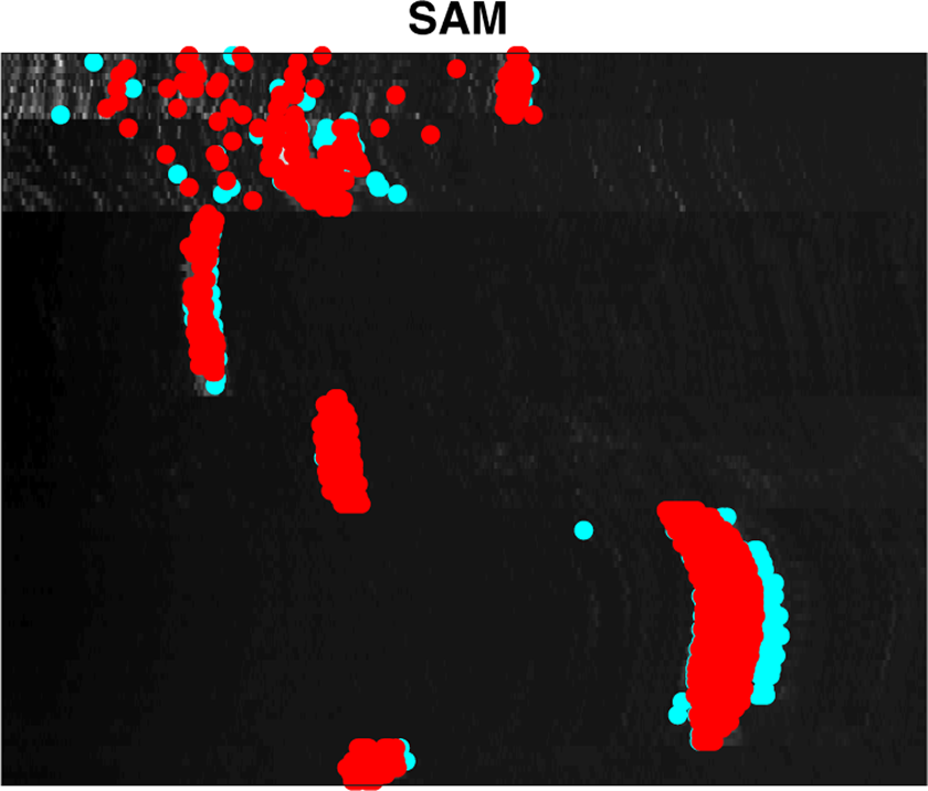
SAM method results—the red points represent the points classified as boat, the blue points represent the light water points and all the points with no color represent the dark water pixels. SAM: Spectral Angle Mapper.

The other images show the results obtained in different phases of the network training. For this, the state of the network was stored after 99, 199, 299, and 399 iterations, and then the prediction for each pixel was performed to be assigned to a class in each stage of the network.

The first line of images shows the ground truth, the results with 99 and 199 iterations, while the second line of images shows the results with 299, 399, and 499 iterations. Taking in consideration the upper left corner of each image, it is possible to observe that in the ground truth image, there are no red dots (boat pixels). However, in the results with 99 and 199 iterations, it is possible to observe red points in the upper left corner. But if we analyze the results of 299, 399, and 499 iterations, these red points disappeared, which shows the improvement with the training evolution of the CNN, by increasing the number of iterations. This will result in more points correctly associated with the correct class.

Table 4 depicts a brief summary of the CNN results.

Table 4.

Summary of CNN results.

	Precision (%)	Recall (%)	F1 Score (%)
Boat	95.38	98.22	96.78
Dark water	97.77	99.98	98.86
Light water	96.96	51.83	67.55

CNN: convolutional neural network.

SAM results

Figure 11 depicts the results for the SAM method, where the red points represent the points classified as boat, while the blue points represent the light water points, and all the points with no color are associated with dark water. In Table 5, we present the precision, recall, and F1 score values obtained for this method.

Table 5.

Summary of SAM method results.

	Precision (%)	Recall (%)	F1 score (%)
Boat	92.17	63.83	75.42
Dark water	93.75	100	96.80
Light water	11.67	10.34	10.97

SAM: spectral angle mapper.

HYDADE results

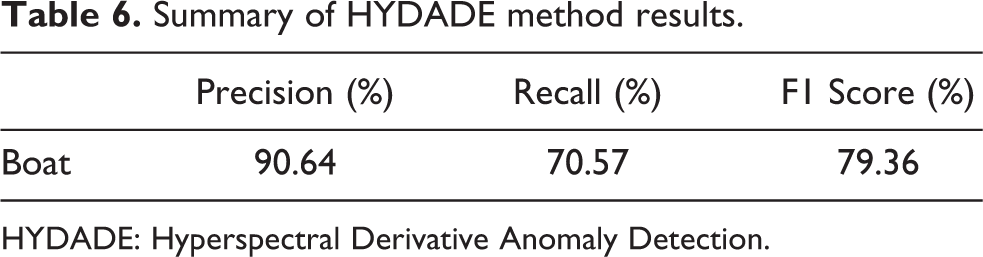
Finally, in Figure 12, we present the results for HYDADE method, where the red points represent the anomaly detection, corresponding to boat points. The other pixels, without any color, represent the water points. It is possible to observe, in the first lines and pixels, that there are some false positives represented mainly because of the sunlight reflection. Despite these external artefacts, the method is able to display accurate results as shown in Table 6.

Figure 12.

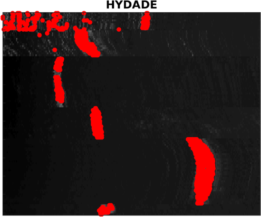
HYDADE method results—the red points represent the points classified as boat. HYDADE: Hyperspectral Derivative Anomaly Detection.

Table 6.

Summary of HYDADE method results.

	Precision (%)	Recall (%)	F1 Score (%)
Boat	90.64	70.57	79.36

HYDADE: Hyperspectral Derivative Anomaly Detection.

Comparing the results of the three methods, it is possible to observe that CNN obtains the higher precision value for all classes. The precision value increases according to the class, being approximately 3% and 5% in relation to SAM and HYDADE, respectively. The dark and light water classes are only used for CNN and SAM, and in the case of the first one, the precision increase using the CNN method compared with SAM method was approximately 4%, while in the light water class, it increased approximately 85%.

However, the effects of the CNN improvements are even more visible in the recall value. For the case of the boat class, the recall value increased approximately 34% when compared to the SAM method and about 27% when compared to the HYDADE method. The dark water class is the only one with higher recall value, when comparing CNN versus SAM approaches. However, the improvement of the SAM method when compared with CNN is only 0.02%. In the case of light water, CNN has an improvement of more than 40% when compared to SAM method.

It is necessary to take into account precision and recall values to evaluate the method performance. A good balance between both metrics indicates best balance between false and true positives. The method that gives the results with both metrics and more balanced is the CNN method, as can be observed in Table 4.

Conclusions and future work

Hyperspectral data classification is always challenging due to the amount of data to be processed. In this work, we implemented three different methods, two supervised (3-D CNN and SAM) and one unsupervised (HYDADE). There are several differences between the three methods, mainly in the training architecture of each one. While supervised methods need to have information about the classes before training, unsupervised methods perform the classification without any prior knowledge about the data.

These differences are reflected in the results obtained, where better results were obtained using supervised methods. The best results were obtained with the 3-D CNN, being possible to notice that this method is more invariant to light and environment changes, although it is the more expensive computational method. The precision and recall values for this method are the most balanced between the three methods, and this balancing can be observed for all the classes.

The results were obtained using a data set collected in the scope of the SUNNY project, in a maritime scenario. During the data set, a surveillance action was simulated with two boats having illegal behaviors. All the data collected were transformed into the radiance domain and then classified using the three different method.

The future work includes testing all methods in different classification scenarios. The implementation of the Nvidia Jetson TX2 already performed will simplify this step and allow an easy integration in future data classification with UAVs.

Footnotes

Declaration of conflicting interests

The author(s) declared no potential conflicts of interest with respect to the research, authorship, and/or publication of this article.

Funding

The author(s) disclosed receipt of the following financial support for the research, authorship, and/or publication of this article: This work is financed by National Funds through the Portuguese funding agency, FCT - Fundação para a Ciência e a Tecnologia within project UID/EEA/50014/2019 and under grant SFRH/BD/139103/2018.

ORCID iD

Sara Freitas

References

Nansen

Zhao

Dakin

. Using hyperspectral imaging to determine germination of native Australian plant seeds. J Photochem Photobiol B Biol 2015; 145: 19–24.

Zhang

Nansen

Aryamanesh

. Importance of spatial and spectral data reduction in the detection of internal defects in food products. Appl Spectrosc 2015; 69(4): 473–480.

Polerecky

Bissett

Al-Najjar

. Modular spectral imaging system for discrimination of pigments in cells and microbial communities. Appl Environ Microb 2009; 75(3): 758–771.

Stein

Schoonmaker

Coolbaugh

. Hyperspectral imaging for intelligence, surveillance and reconnaissance. Space and Naval Warfare Systems Center Command, San Diego, CA, 2001.

Freitas

Silva

Almeida

. Hyperspectral imaging for real-time unmanned aerial vehicle maritime target detection. J Intell Robot Syst 2018; 90(3): 551–570.

SUNNY Project. Online Referencing, http://www.sunnyproject.eu (2014, accessed 10 October 2018).

Chen

Lin

Zhao

. Deep learning-based classification of hyperspectral data. IEEE J Sel Top Appl Earth Obs Remote Sens 2014; 7(6): 2094–2107.

Huang

Wei

. Deep convolutional neural networks for hyperspectral image classification. J Sens 2015; 2015: 1–12.

Zhao

. Spectral-spatial feature extraction for hyperspectral image classification: a dimension reduction and deep learning approach. IEEE Trans Geosci Remote Sens 2016; 54(8): 4544–4554.

10.

Chen

Jiang

. Deep feature extraction and classification of hyperspectral image based on convolutional neural networks. IEEE Trans Geosci Remote Sens 2016; 54: 6232–6251.

11.

Liu

Zhang

Eom

. Active deep learning for classification of hyperspectral images. IEEE J Sel Top Appl Earth Obs Remote Sens 2017; 10(2): 712–724.

12.

Zhong

Gong

. Learning to diversify deep belief networks for hyperspectral image classification. IEEE Trans Geosci Remote Sens 2017; 55(6): 3516–3530.

13.

Chen

Zhao

Jia

. Spectral-spatial classification of hyperspectral data based on deep belief network. IEEE J Sel Top Appl Earth Obs Remote Sens 2015; 8(6): 2381–2392.

14.

Zhang

. Classification of hyperspectral image based on deep belief networks. IEEE Image Proc 2014; 5132–5136.

15.

Farrell

Mersereau

. On the impact of PCA dimension reduction for hyperspectral detection of difficult targets. IEEE Geosci Remote Sens Lett 2005; 2(2): 192–195.

16.

Zhong

Gong

Schönlieb

. A diversified deep belief network for hyperspectral image classification. Int Arch Photogram Remote Sens Spatial Inform Sci 2016; XLI-B7: 443–449.

17.

Lee

Kwon

. Going deeper with contextual CNN for hyperspectral image classification. IEEE Trans Image Process 2017; 26(10): 4843–4855.

18.

Zhang

. Spectral-spatial classification of hyperspectral imagery using a dual-channel convolutional neural network. Remote Sens Lett 2017; 8(5): 438–447.

19.

Parkhi

Vedaldi

Zisserman

. A deep face recognition. In Proceedings of the British machine vision. 2015.

20.

Lawrence

Giles

Tsoi

. Face recognition: a convolutional neural-network approach. IEEE Trans Neural Networ 1997; 8(1): 98–113.

21.

Ren

Girshick

. Faster r-cnn: towards realtime object detection with region proposal networks. IEEE Trans Pattern Anal 2017; 39: 1137–1149.

22.

Karpathy

Toderici

Shetty

. Large-scale video classification with convolutional neural networks. In: Proceedings of the IEEE international conference on computer vision and pattern recognition 2014.

23.

Jia

. Convolutional neural networks for hyperspectral image classification. Neurocomputing 2017; 219: 88–98.

24.

Paoletti

Haut

Plaza

. A new deep convolutional neural network for fast hyperspectral image classification. ISPRS J Photogramm 2018; 145: 120–147.

25.

Liu

Sun

Liu

. Hyperspectral image classification based on convolutional neural network and dimension reduction. In: 2017 Chinese automation congress (CAC), Jinan, 2017, pp. 1686–1690. DOI: 10.1109/CAC.2017.8243039.

26.

Zang

Zhang

. A review of remote sensing image classification techniques: the role of spatio-contextual information. Eur J Remote Sens 2014; 47: 389–411.

27.

Zhang

. Deep learning for remote sensing data advances in machine learning for remote sensing and geosciences. IEEE Geosci Remote Sens Mag 2016; 4: 22–40.

28.

Ghamisi

Plaza

Chen

. Advanced supervised spectral classifiers for hyperspectral images: a review. IEEE Geosci Remote Sens Mag 2017; 5: 8–32.

29.

Xia

. Transferring deep convolutional neural networks for the scene classification of high-resolution remote sensing imagery in surveying, mapping and remote sensing. Remote Sens 2015; 7: 14680–14707.

30.

Salinas Hyperspectral Remote Sensing Scenes. Grupo de Inteligencia Computacional. Online Referencing, http://www.ehu.eus/ccwintco/index.php/Hyperspectral_Remote_Sensing_Scenes#Salinas (2014, accessed 2 October 2018).

31.

Baumgardner

Marion F.

Biehl

Larry L.

Landgrebe

David A.

220 Band AVIRIS Hyperspectral Image Data Set: June 12, 1992 Indian Pines Test Site 3. Online Referencing, http://www.ehu.eus/ccwintco/index.php/Hyperspectral_Remote_Sensing_Scenes#Indian_Pines (2014, accessed 2 October 2018).

32.

Pavia Centre and University. Grupo de Inteligencia Computacional. Online Referencing, http://www.ehu.eus/ccwintco/index.php/Hyperspectral_Remote_Sensing_Scenes#Pavia_Centre_and_University (2014, accessed 2 October 2018).

33.

Yue

Zhao

Mao

. Spectral–spatial classification of hyperspectral images using deep convolutional neural networks. Remote Sens Lett 2015; 6: 468–477.

34.

Gao

Lim

Jia

. Hyperspectral image classification using convolutional neural networks and multiple feature learning. Remote Sens 2018; 10(2): 299.

35.

Kruse

Lefkoff

Boardman

. The spectral image processing system (sips)—interactive visualization and analysis of imaging spectrometer data. Remote Sens Environ 1993; 44(2): 145–163.

36.

LeCun

Bengio

learning

GHD

. Deep learning. Nature 2015; 521: 436–444.

37.

Jarrett

Kavukcuoglu

Ranzato

. What is the best multistage architecture for object recognition? In: IEEE international conference on computer vision (ICCV), Vision, Kyoto, 2009, pp. 2146–2152.

38.

Nair

Hinton

. Rectified linear units improve restricted Boltzmann machines. In: Proceedings of the 27th international conference on machine learning, 2010, pp. 807–814.

39.

Glorot

Bordes

Bengio

. Deep sparse rectifier neural networks. In: Proceedings of the fourteenth international conference on artificial intelligence and statistics (AISTATS-11) journal of machine learning research – workshop and conference proceedings, USA, 11–13 April 2011, pp. 315–323.

40.

Glorot

Bengio

. Understanding the difficulty of training deep feedforward neural networks. In: Proceedings of the international conference on artificial intelligence and statistics (AISTATS10), Chia Laguna Resort, Sardinia, Italy, 13–15 May 2010, pp. 249–256.

41.

Duchi

Edu

Hazan

. Adaptive subgradient methods for online learning and stochastic optimization. J Mach Learn Res 2011; 12: 2121–2159.

42.

TensorFlow. Online Referencing, https://www.tensorflow.org/ (2015, accessed 11 October 2018).

43.

Garcia

. Learning from imbalance data. IEEE Trans Knowl Data En 2009; 21(9): 1263–1284.

Convolutional neural network target detection in hyperspectral imaging for maritime surveillance

Abstract

Keywords

Introduction

Related work

Hyperspectral payload UAV integration and data collection

Hyperspectral cameras

Spectrum processing

Target detection methods

Deep CNN

Spectral angle mapper

Hyperspectral derivative anomaly detection

Results

Flight experiment

CNN results

SAM results

HYDADE results

Conclusions and future work

Footnotes

Declaration of conflicting interests

Funding

ORCID iD

References