Sage Journals: Discover world-class research

Abstract

The boundary layer state has a critical effect on hypersonic vehicle performance and the noise level is the main factor causing the differences between the boundary layer transition in a wind tunnel test and that in a real flight. The second mode wave frequency of the 7° half-angle cone models as measured in four hypersonic wind tunnels is collected. The effects of the noise level on the boundary layer are determined by comparing dimensionless parameters, which are nondimensionalized based on computed values. The results indicate that the noise level could affect the second mode wave frequency and the boundary layer thickness, where the second mode wave frequency decreases and the boundary layer thickness increases with increasing noise level. However, the mechanism by which the noise level influences the second mode wave frequency and the boundary layer thickness requires further study.

Keywords

Hypersonic flow boundary layer transition noise level second mode wave frequency boundary layer thickness cone model

Introduction

The hypersonic boundary layer transition has a dramatic effect on skin friction, heat transfer rates, and flow separation, and thus influences the aerodynamic, aerothermal, stability, inlet starting, and burning performances of hypersonic vehicles. The laminar-turbulent transition prediction has been one of the main factors limiting the development of hypersonic vehicles.^1–7

The boundary layer transition is a complex nonlinear phenomenon that is strongly affected by multiple factors, including freestream disturbances, the Mach number, the Reynolds number, the angle of attack, the wall temperature, leading edge bluntness, the wall roughness, and wall catalysis.^8,9 The current prediction accuracy for the hypersonic boundary layer transition is seriously insufficient. Bertin and Cummings¹⁰ noted that none of the semi-empirical models that have predicted the boundary layer transition position accurately under different flight conditions had been obtained within the past 50 years. In summing up the history of research into the hypersonic boundary layer transition, Bushnell¹¹ stated that researchers have not yet succeeded in predicting the hypersonic (or even supersonic) boundary layer transition. Schneider¹² counted large quantities of flight test data and found that although the distribution of the boundary layer transition Reynolds number in flight tests was similar to that obtained from ground wind tunnel test data, the divergence was very high, even ranging up to a difference of one order of magnitude.

In hypersonic flow, the noise level, which is the ratio of the root mean square of the fluctuating pressure to the mean pressure, is used widely to characterize the flow disturbance. The noise level is an important factor in determining the major differences between the boundary layer transition Reynolds numbers of different hypersonic wind tunnels, and is also a factor in the differences between wind tunnel tests and flight tests. Under hypersonic conditions, the noise level differences between the hypersonic wind tunnel test conditions and those of a real flight environment are significant, and may even extend one to two orders of magnitude.¹³ The noise level not only affects the transition path of the hypersonic boundary layer but also has been shown to have a significant influence on the bluntness effect,¹⁴ the attack angle effect,^15,16 the roughness effect, the second mode disturbances,¹⁷ the transition zone length,^14,18 and cross-flow instability.^19,20 Therefore, most of the transition data obtained from hypersonic wind tunnel tests under high noise level conditions are likely to be invalid.⁸ To study hypersonic boundary layer transitions under low noise level conditions, hypersonic quiet wind tunnels were developed.^13,21,22 Although the noise level in these tunnels is much lower than that in a conventional hypersonic wind tunnel, the noise level is still higher than that in a real flight environment. In addition, because of the limited ranges available for the Mach number, the nozzle dimensions, and the Reynolds number, it is difficult for the hypersonic quiet wind tunnel to meet the requirements of hypersonic vehicle boundary layer transition testing. Conventional hypersonic wind tunnels, which have wide simulation ranges and high noise levels, thus continue to play an irreplaceable role in hypersonic boundary layer transition research.

It should be noted here that previous studies of the noise level effect were mainly in the form of qualitative analyses, which produced results that cannot be applied directly to hypersonic boundary layer prediction under real flight conditions. For this reason, the influence of the hypersonic flow noise level on the boundary layer is studied further here, and the quantitative relationship between the hypersonic flow noise level and the boundary layer thickness is thus established.

Research method

Numerical calculations, wind tunnel tests, and flight tests are the three major means of aerodynamic research. In studies of the noise level effect, numerical calculations cannot fully simulate the real free disturbances in the hypersonic wind tunnel. A hypersonic wind tunnel cannot generate different noise levels for the flow conditions while maintaining the other flow parameters at the same levels, and flight tests cannot obtain sufficient flow and boundary layer information. There is thus a lack of a direct means with which to study the noise level effects of hypersonic wind tunnels.

Because of the lack of a high-precision hypersonic boundary layer thickness measurement method, the second mode wave frequency of a 7° half-angle cone model that is measured in four hypersonic wind tunnels is collected to study the effects of the noise level on the boundary layer. As shown in Figure 1, based on the relationship between the second mode wave frequency and the boundary layer thickness,²³ the boundary layer thicknesses in the hypersonic wind tunnels with the different noise levels are converted using this indirect method and are then compared with the numerical calculation results. The effects of the hypersonic wind tunnel noise level on the boundary layer thickness can then be obtained.

Figure 1.

Diagram of the research method used.

First, the boundary layer thickness δ_CFD (0.99) and the boundary layer edge velocity U_e of the cone model are calculated under different flow conditions using a computational fluid dynamics (CFD) approach. Then, based on the relationship between the second mode wave frequency, the boundary layer edge velocity, and the boundary layer thickness, the computed second mode wave frequency f_2nd-CFD can be determined, and the value obtained is confirmed by the result of the linear stability analysis. Finally, by using f_2nd-CFD as a reference value, the dimensionless second mode wave frequency f_2nd-EXP/f_2nd-CFD is calculated, and the noise level effect on the second mode wave frequency can then be obtained.

Similarly, the values of the boundary layer thickness δ_EXP are computed using the measured second mode wave frequency f_2nd-EXP and the calculated boundary layer edge velocity U_e from the simulations. Using the simulated boundary layer thickness δ_CFD as a reference value, the dimensionless boundary layer thicknesses δ_EXP/δ_CFD are determined, and the noise level effect on the boundary layer thickness can then be obtained.

The second mode wave frequency values measured in the different hypersonic wind tunnels can reflect the influence of the noise level. The boundary layer thicknesses at different locations in the different hypersonic wind tunnels can also be compared with the calculated boundary layer thickness values.^24–27

Experimental data

Experimental data were obtained from four hypersonic wind tunnels: hypersonic quiet wind tunnel BAM6QT,²⁴ conventional hypersonic wind tunnel H2K,²⁵ shock tunnel JF-8A,²⁶ and shock tunnel FD-14A.²⁷ The noise levels of the four wind tunnels ranged from 0.05% to 4.5%. Table 1 lists the experimental data obtained.

Table 1.

Experimental results from hypersonic wind tunnels.

Case no.	Wind tunnel	Test gas	Mach number (Ma)	SR ¹ (mm)	Noise level	Location²	f _2nd-EXP (kHz)
Case 1	BAM6QT-RUN21	Air	6	0	≈0.05%	X=340 mm	217.2
Case 2	BAM6QT-RUN21	Air	6	0	≈0.05%	X=390 mm	202
Case 3	BAM6QT-RUN26	Air	6	0	≈0.05%	X=340 mm	237
Case 4	BAM6QT-RUN26	Air	6	0	≈0.05%	X=390 mm	221.4
Case 5	BAM6QT-RUN35	Air	5.8	0	≈3%	X=340 mm	214.5
Case 6	BAM6QT-RUN35	Air	5.8	0	≈3%	X=390 mm	199.5
Case 7	BAM6QT-RUN11	Air	5.8	0	≈3%	X=340 mm	228.5
Case 8	BAM6QT-RUN11	Air	5.8	0	≈3%	X=390 mm	212.2
Case 9	JF-8A	Air	6.5	0	≈2.8%	X=405 mm	206
Case 10	H2K	Air	7	1.6	≈3%	X=399.1 mm	236
Case 11	H2K	Air	7	1.6	≈3%	X=456.1 mm	221
Case 12	FD-14A	N₂	10	0.05	≈4.5%	X=285 mm	342.8
Case 13	FD-14A	N₂	10	0.05	≈4.5%	X=365 mm	290
Case 14	FD-14A	N₂	10	0.05	≈4.5%	X=445 mm	272.5

¹SR: cone tip radius.

²The origin is located at the tip of the cone model.

Because the noise level of the H2K wind tunnel could not be found in the published literature, its noise level was determined by comparing the boundary layer transition Reynolds numbers for the cone model in the H2K and FD-07 wind tunnels.^25,28,29

Numerical calculations

Numerical simulations are generally conducted in this field for two purposes. The first purpose is to determine the boundary layer outer edge velocity U_e and then calculate the boundary layer thickness δ_EXP using the measured second mode wave frequency f_2nd-EXP. Second, the computed boundary layer thickness δ_CFD is selected as a reference value that can then be used to nondimensionalize the boundary layer thickness at different locations in various wind tunnels.

Computational method

The second-order upwind finite volume method is used to solve the boundary layer equation and the laminar flow field of the cone model at a 0° angle of attack is then obtained. Figure 2 presents the computation domain, where the axisymmetric boundary condition is applied to simplify the three-dimensional flow field to the two-dimensional case. The cone tip has two configurations. When SR>0, the cone has a blunt tip with radius SR, and the case where SR=0 represents a sharp cone tip. The inlet and outlet are both far-field pressure conditions, the model wall is isothermal, and the wall temperature is T_w=300 K. Either ideal air or nitrogen is used, which is the same as the wind tunnel test gas conditions. The computational mesh is shown in Figure 3. The grids in the areas close to the wall and to the tip are denser to aid in resolving the shock wave and the boundary layer accurately.

Figure 2.

Computational domain.

Figure 3.

Computation mesh (SR=1.6 mm).

Mesh independence

Three mesh sizes were used to calculate the flow field around the cone model.²⁶ The flow conditions for the numerical calculations are consistent with those of the wind tunnel test and the mesh details are as listed in Table 2. The streamwise velocity profiles at X =405 mm obtained from the numerical simulations using three different meshes are shown in Figure 4. The three velocity profiles are basically the same, and a mesh of 1550×200 is selected for use in the subsequent numerical calculations.

Table 2.

Computational mesh details.

Mesh no.	Streamwise velocity component (m/s)	Spanwise velocity component (m/s)
1	900	130
2	1550	200
3	1620	270

Figure 4.

Spanwise velocity profile (X=405 mm).

Method validation

To provide further validation of the calculation method, the high-precision WENO5 scheme was used to calculate the flow fields of Run 21 and Run 11 in the BAM6QT tunnel,²⁴ and the boundary layer thickness and boundary layer edge velocity were then obtained. The growth rates of the perturbation waves (α_i) at X=340 mm and X=390 mm were studied by performing a linear stability analysis. The second mode wave frequencies were acquired and the results are shown in Table 3 and Figure 5. The boundary layer edge velocities calculated using these two schemes are very close but the boundary layer thickness calculated using the WENO5 scheme was a little thinner, with a difference of less than 10%. Furthermore, the values of the second mode wave frequencies, which are the frequencies of the most unstable perturbation waves, were obtained using the linear stability analysis and the empirical equation (1), and the calculated values are nearly the same. Therefore, the second-order upwind scheme was selected to study the boundary layer thickness of the cone model hereinafter.

Table 3.

Calculation results for the cone boundary layer in wind tunnel BAM6QT.

Run	Location	U _e (m/s)	U _e-WENO5 (m/s)	δ _CFD (mm)	δ _CFD-WENO5 (mm)	f _2nd-CFD ¹ (kHz)	f _2nd-LST ² (kHz)	f _2nd-EXP (kHz)
Run 21	X=340 mm	842.15	842.5	1.91	1.73	176.4	188.4	217.2
Run 21	X=390 mm	842.15	842.5	2.02	1.86	166.8	175.7	202
Run 11	X=340 mm	920.3	920.73	1.53	1.44	240.6	240.7	228.5
Run 11	X=390 mm	920.3	920.73	1.60	1.54	230.1	223.7	212.2

¹f _2nd-CFD=0.4×U_e/δ_CFD.

²f _2nd-LST is obtained using the linear stability analysis method.

Figure 5.

Perturbation wave growth rates.

The second mode wave frequency f_2nd can be estimated using equation (1):²³

f_{2 nd} \approx 0.4 \frac{U_{e}}{δ}

(1)

where U_e is the laminar boundary layer edge velocity and δ is the laminar boundary layer thickness.

To compare the simulation method with the empirical formula, the cone model flow field is simulated using the method from the literature.²⁶U_e is 1039.4 m/s at the location X=405 mm, and δ is 1.79 mm. The second mode wave frequency estimated using equation (1) is 232.3 kHz, which is very close to the actual measured frequency of 206 kHz, showing a difference of less than 13%. Similarly, the cone model flow field is also calculated as shown in the literature²⁴ (Run 11), where U_e is 920.3 m/s at the location X=340 mm and δ is 1.53 mm. The second mode wave frequency estimated using equation (1) in this case is 240.6 kHz, which is very close to the measured frequency of 228.5 kHz, showing a difference of less than 6%. The estimated second mode wave frequencies are thus consistent with the experimental results.

Tip radius effect

The tip radius of the sharp cone model may vary slightly because of variations in the machining tolerance. Given that the model tip’s bluntness may potentially influence the boundary layer properties, the velocity profiles of cone models with different tip radii (SR=0 mm and SR=0.05 mm) were acquired via numerical simulations, where the flow conditions were the same as those of Run 21 in reference [24]. The resulting velocity profiles are compared in Figure 6, which shows that the tip radius hardly affects the boundary layer. In the subsequent calculations for the sharp tip cone model, the tip radius is defined as SR=0 mm without consideration of the machining tolerance.

Figure 6.

Velocity profiles of the cone models with different tip radii.

Results and discussion

The same grid topology, grid number, and computation method are used to calculate the laminar flow field under four different flow conditions (see Table 4) in BAM6QT and using the two operating modes given in reference [24]. The boundary layer thicknesses and boundary layer edge velocities at the two positions at X=340 mm and X=390 mm are determined, and the second mode wave frequencies are then calculated based on the relationship between the boundary layer thickness and the second mode wave frequency.²³ Table 5 lists the calculated and measured results for the second mode wave frequency and the boundary layer thickness. The test conditions for Run 35 and Run 21 are similar, and those of Run 26 are similar to those of Run 11. The results show that without the noise level effect, the calculated laminar boundary layer thickness of Run 35 is thinner when compared with that of Run 21, and the second mode wave frequency of Run 35 is also higher. However, the measured second mode wave frequency for Run 35 is lower than that for Run 21. Additionally, the second mode wave frequencies of Run 26 and Run 11 show the same trend. It is therefore speculated that the flow noise level has effects on both the laminar boundary layer thickness and the second mode wave frequency. The second mode wave frequency decreases and the laminar boundary layer thickness increases with increasing noise level.

Table 4.

Test conditions for BAM6QT.²⁴

Run no.	Flow	Noise level	Test gas	Ma	P ₀ (MPa)	T ₀ (K)
Run 21	Quiet flow	≈0.05%	Air	6	0.616	415
Run 26	Quiet flow	≈0.05%	Air	6	0.763	418
Run 35	Noisy flow	≈3%	Air	5.8	0.567	416
Run 11	Noisy flow	≈3%	Air	5.8	0.794	500

Table 5.

Calculated and measured results for the second mode wave frequency and the boundary layer thickness under the test conditions for BAM6QT.

Run no.	Location	U _e (m/s)	δ _CFD (mm)	f _2nd-CFD (kHz)	f _2nd-EXP (kHz)	δ _EXP (mm)¹	Δδ² (mm)	δ _EXP/δ_CFD
Run 21	X=340 mm	842.15	1.91	176.4	217.2	1.55	−0.36	0.81
Run 21	X=390 mm	842.15	2.02	166.8	202	1.67	−0.35	0.83
Run 26	X=340 mm	845.3	1.68	201.3	237	1.43	−0.25	0.85
Run 26	X=390 mm	845.3	1.77	191.0	221.4	1.53	−0.24	0.86
Run 35	X=340 mm	839.3	1.87	179.5	214.5	1.57	−0.30	0.84
Run 35	X=390 mm	839.3	1.88	178.6	199.5	1.68	−0.20	0.90
Run 11	X=340 mm	920.3	1.53	240.6	228.5	1.61	0.08	1.05
Run 11	X=390 mm	920.3	1.60	230.1	212.2	1.73	0.13	1.08

¹δ _EXP = 0.4×U_e/f_2nd-EXP.

²Δδ=δ_EXP−δ_CFD.

To provide further confirmation of the influence of the noise level on the boundary layer thickness and the second mode wave frequency, the laminar flow fields of three wind tunnels, comprising JF8A,²⁶ H2K,²⁵ and FD-14A,²⁷ are calculated using the same grid topology, the same grid number, and the same computational method. Table 6 lists the flow conditions, and the computational and experimental results for the second mode wave frequency and the boundary layer thickness are presented in Table 7. The calculated second mode wave frequencies are higher than the measured values in the quiet flow cases (Run 21 and Run 26 for BAM6QT). However, the calculated second mode wave frequencies are lower than the measured values obtained under noisy flow conditions. The relationship between the dimensionless second mode wave frequency and the noise level is plotted in Figure 7, and the relationship between the dimensionless boundary layer thickness and the noise level is plotted in Figure 8. The dimensionless second mode wave frequency decreases and the dimensionless boundary layer thickness increases when the noise level increases.

Table 6.

Test conditions of the hypersonic wind tunnels.

Wind tunnel	Noise level	Test gas	Ma	P ₀ (MPa)	T ₀ (K)
JF8A²⁶	≈2.8%	Air	6.5	1.2	620
H2K²⁵	≈3%	Air	7	2.33	600.9
FD-14A²⁷	≈4.5%	N₂	10	352	44

Table 7.

Calculated and measured results for the second mode wave frequency and the boundary layer thickness under the conditions in the JF8A, H2K, and FD-14A wind tunnels.

Wind tunnel	Location	U _e (m/s)	δ _CFD (mm)	f _2nd-CFD (kHz)	f _2nd-EXP (kHz)	δ _EXP (mm)	Δδ (mm)	δ _EXP/δ_CFD
JF8A	X=405 mm	1039.4	1.79	232.3	206	2.02	0.23	1.13
H2K	X=399.1 mm	1031.8	1.59	259.6	236	1.75	0.16	1.10
H2K	X=456.1 mm	1031.8	1.69	244.2	221	1.87	0.18	1.11
FD-14A	X=285 mm	1336.25	1.21	441.7	342.8	1.56	0.35	1.29
FD-14A	X=365 mm	1336.25	1.42	376.4	290	1.84	0.42	1.30
FD-14A	X=445 mm	1336.25	1.44	371.2	272.5	1.96	0.52	1.36

Figure 7.

Second mode wave frequency vs. noise level characteristics.

Figure 8.

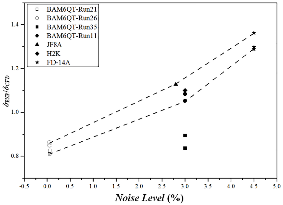
Boundary layer thickness vs. noise level characteristics.

The dimensionless second mode wave frequency is linearly correlated with the noise level, with the exception of the case of Run 35 in BAM6QT. The linear relationship between the second mode wave frequency ratio and the noise level is obtained by least squares fitting; see equation (2). Note here that the Run 35 data were not used in the fitting.

f_{2 nd - EXP} / f_{2 nd - CFD} = 1.19994 - 9.709 * Noise level

(2)

Figure 9 shows the relationship between the noise level and the boundary layer thickness difference. The boundary layer thickness difference can be obtained by subtracting the calculated boundary layer thickness value from the measured value, and the measured boundary layer thickness is converted using equation (1). The calculated boundary layer thicknesses are acquired using the same grid topology, grid numbers, and calculation method. The boundary layer thickness differences increase when the noise level increases, and the boundary layer thickness difference basically increases linearly with the noise level, except in the case of Run 35 in BAM6QT. The functional relationship between the boundary layer thickness difference and the noise level is acquired using a least squares fitting approach; see equation (3).

δ_{EXP} - δ_{CFD} = - 0.31179 + 16.181 * Noise level

(3)

Figure 9.

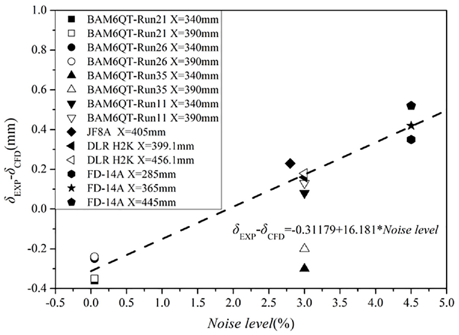
Boundary layer thickness difference vs. noise level characteristics.

Conclusions

To study the effects of noise levels on the hypersonic boundary layer, the second mode frequencies of 7° half-angle cone models measured in four hypersonic wind tunnels have been collected. The boundary layer thicknesses and boundary layer edge velocities were obtained by performing numerical simulations under various flow conditions. Based on the relationship between the second mode wave frequency and the boundary layer thickness, the wind tunnel boundary layer thicknesses are obtained by using the measured second mode wave frequencies. The second mode wave frequency and boundary layer thickness values are nondimensionalized using computed values. The results show that the noise level could affect both the second mode wave frequency and the boundary layer thickness. Specifically, the second mode wave frequency decreases and the boundary layer thickness increases when the noise level increases.

In this paper, an empirical equation for the boundary layer thickness, which is difficult to measure immediately in wind tunnel experiments, is proposed for the first time. By measuring the second mode frequency, the boundary layer thickness can be evaluated with respect to the noise level in wind tunnel experiments. This result is of considerable practical significance; for example, it could enable the design of a boundary layer strip with a height that is related to the boundary layer thickness and enable boundary layer transition prediction for real flights using wind tunnel test data. The results indicate that the noise level has an effect on both the second mode wave frequency and the laminar boundary layer thickness; however, the mechanism by which the noise level influences the second mode wave frequency and the boundary layer thickness will require further study in future work.

Footnotes

Handling Editor: Chenhui Liang

Declaration of conflicting interests

The author(s) declared no potential conflicts of interest with respect to the research, authorship, and/or publication of this article.

Funding

The authors disclosed receipt of the following financial support for the research, authorship, and/or publication of this article: The authors would like to acknowledge the support of the National Key R&D Program of China (2019YFA0405300) and the National Natural Science Foundation of China (U20B2003, 92152301).

ORCID iD

Xinguo Sha

References

Duan

Chen

. Some aerodynamic issues in hypersonic flight. Acta Aeronaut Astronaut Sin 2015; 36: 7–23.

Zhou

Zhang

. Two problems in the transition and turbulence for near space hypersonic flying vehicles. Acta Aerodyn Sin 2017; 35: 151–155.

Zhang

Jiang

, et al. Some key problems in the study of aerodynamic characteristics of near-space hypersonic vehicles. Chinese Journal of Theoretical and Applied Mechanics 2018; 50: 1292–1310.

Yuan

Huang

, et al. A perspective of system engineering on hypersonic boundary-layer transition. Acta Aerodyn Sin 2021; 39: 26–38.

Reshotko

. Transition issues for atmospheric entry. J Spacecr Rockets 2015; 45: 161–164.

, et al. Key issues in hypersonic vehicle aerodynamic design. Sci Sin Phys Mech Astron 2021; 51: 6–25.

Chen

Yuan

, et al. Progress in flight tests of hypersonic boundary layer transition. Acta Mech Sin 2021; 37: 1591–1611.

Chen

Zhang

, et al. Hypersonic boundary layer transition: What we know, where shall we go. Acta Aerodyn Sin 2017; 35: 311–337.

Chen

Yuan

, et al. Recent progresses on hypersonic boundary-layer transition. Sci Sin Phys Mech Astron 2019; 49: 125–138.

10.

Bertin

Cummings

. Fifty years of hypersonics: Where we’ve been, where we’re going. Prog Aerosp Sci 2003; 39: 511–536.

11.

Bushnell

. Hypersonic flight experimentation – Status and shortfalls. In: Future aerospace technology in the service of the alliance, Vol. 3. 1997.

12.

Schneider

. Flight data for boundary-layer transition at hypersonic and supersonic speeds. J Spacecr Rockets 2011; 36: 8–20.

13.

Schneider

. Development of hypersonic quiet tunnels. J Spacecr Rockets 2008; 45: 641–664.

14.

Chen

F-J

. Boundary-layer transition extent measurements on a cone and flat plate at Mach 3.5. In: Proceedings of the 31st aerospace sciences meeting, Reno, NV, USA, 11–14 January 1993. AIAA.

15.

King

R A

. Three-dimensional boundary-layer transition on a cone at Mach 3.5. Exp Fluids 1992; 13: 305–314.

16.

Stetson

. Mach 6 experiments of transition on a cone at angle of attack. J Spacecr Rockets 2015; 19: 397–403.

17.

Pate

. Supersonic boundary-layer transition – Effects of roughness and freestream disturbances. AIAA Journal 1971; 9: 797–803.

18.

Harvey

Bobbitt

. Some anomalies between wind tunnel and flight transition results. In: 14th fluid and plasma dynamics conference, Palo Alto, CA, USA, 23–25 June 1981. AIAA.

19.

Borg

Kimmel

Stanfield

. Traveling crossflow instability for the HIFiRE-5 elliptic cone. J Spacecr Rockets 2015; 52.

20.

Borg

Kimmel

. Simultaneous infrared and pressure measurements of crossflow instability modes for HIFiRE-5. In: Proceedings of the AIAA aerospace sciences meeting, San Diego, CA, USA, 4–8 January 2016. AIAA.

21.

Gang

. Design and performance of a hypersonic quiet wind tunnel at NUDT. In: Proceedings of the 21st AIAA international space planes and hypersonics technologies conference, Xiamen, China, 6–9 March, 2017. AIAA.

22.

Lee

Chen

. Recent progress in the study of transition in the hypersonic boundary layer. Natl Sci Rev 2019; 6: 155–170.

23.

Stetson

. Hypersonic boundary-layer transition. In: Bertin

Periaux

Ballmann

(eds) Advances in Hypersonics: Defining the Hypersonic Environment, vol. 1. Boston: Birkhäuser, 1992, pp. 324–417.

24.

Estorf

Radespiel

Schneider

, et al. Surface-pressure measurements of second-mode instability in quiet hypersonic flow. In: Proceedings of the 46th AIAA aerospace sciences meeting and exhibit, Reno NV, USA, 7–10 January 2007. AIAA.

25.

Willems

Gülhan

Juliano

, et al. Laminar to turbulent transition on the HIFiRE-1 cone at Mach 7 and high angle of attack. In: Proceedings of the 52nd aerospace sciences meeting, National Harbor, MD, USA, 13–17 January 2014. AIAA.

26.

Wang

, et al. Experimental study on stability and transition of sharp cone hypersonic boundary layer. Journal of Beijing University of Aeronautics and Astronautics 2020; 46: 2087–2093.

27.

Jiang

Chen

, et al. Measurement technique and application of boundary layer transition in shock tunnel. Acta Aeronaut Astronaut Sin 2019; 40: 66–77.

28.

Xie

. Study of phenomenon, mechanism and effect of hypersonic shock wave/transitional boundary layer interaction. PhD Thesis: China Academy of Aerospace Aerodynamics, Beijing, China, 2015.

29.

Sha

Guo

, et al. Experimental study on instability streak structure over a hypersonic cone. Acta Aerodyn Sin 2020; 38: 143–147.

Noise level effect on the hypersonic boundary layer

Abstract

Keywords

Introduction

Research method

Experimental data

Numerical calculations

Computational method

Mesh independence

Method validation

Tip radius effect

Results and discussion

Conclusions

Footnotes

Declaration of conflicting interests

Funding

ORCID iD

References