A decentralized approach to formation flight routing of long-haul commercial flights

Abstract

This paper describes the development of an optimization-based cooperative planning system for the efficient routing and scheduling of extended flight formations. This study considers the use of formation flight as a means to reduce the overall fuel consumption in long-haul airline operations. It elaborates on the operational implementation of formation flight, particularly focusing on the formation flight routing. A completely decentralized approach is presented, in the sense that formation flight is not planned pre-flight and is not subjected to any predefined routing restrictions. A greedy communication scheme is defined through which all participating aircraft are allowed to communicate with neighboring aircraft in order to establish flight formations in flight. A constraint on the formation-flight-induced additional flight time is introduced in order to suppress the occurrence of large detours in the assembly of flight formations. A transatlantic case study is presented that considers 347 eastbound flights. Assuming a 10% fuel flow reduction for any trailing aircraft in a formation, the overall network-wide fuel savings were estimated at 4.3% at the expense of an additional flight time of 10.3 min per flight on average. In this transatlantic long-haul scenario, a formation flight usage rate of 73% was realized.

Introduction

Over the past decades, formation flight has become a recognized method when considering possibilities to improve the fuel efficiency in civil aviation. Compared to other efficiency measures, such as innovative aircraft designs, formation flight requires a limited amount of new technology, as potential implementation largely boils down to regulatory and operational changes.

By examining the flight behavior of birds, as done by Lissaman in 1970, ¹ a general understanding of the (aero)dynamics of formation flight was developed and application of flight formation to fixed-wing aircraft was subsequently proposed. As the potential for fuel savings due to induced drag reductions of trailing aircraft in an “extended” formation became more apparent, flight tests were conducted to confirm this finding, ² and more recently in Flanzer and Bieniawski. ³ The latter study considered formation flight of two military C-17 aircraft and fuel savings of 5–10% were reported for the trailing aircraft, increasing with mission length. Note that in an extended formation aircraft are longitudinally separated by 5–40 wingspans. ⁴

To capitalize on the acquired knowledge in the context of airline operations, the planning of formation flights on a network-wide scale has been explored. In Ribichini and Frazzoli, ⁵ an approach to the formation flight routing for unmanned aerial vehicles is presented. In this study, a greedy algorithm is applied that considers formation flight as an in-flight option. This locally coordinated use of formation flight characterizes what is known as a decentralized approach. The authors clearly demonstrate that one of the main advantages of the decentralized approach that they propose is that flight (departure) delays can be readily accommodated, as delayed aircraft are simply able to search alternative formation flight partners within the network. A major downside of their decentralized approach is that the global fuel-savings potential of flight formation is not fully exploited, due to the greedy nature of the flight formation assembly decision-making process.

Another interesting effort towards decentralized organization of civil formation flight has been made by Xue et al., ⁶ who considered the use of corridors in the sky over North America within which each flight would be routed. While residing in a corridor, flights are allowed to adjust their speed in order to facilitate the assembly of a formation. The authors show that their approach makes it possible to manage delayed flights by simply linking them up with alternative formation partners within the corridors. However, redirecting all flights through the corridors requires a significant fuel investment for all aircraft, without having a guarantee that they will all be included in a formation.

In recent years, the focus in research on network-wide formation flight planning has shifted to the concurrent routing and assignment of formation flights for an entire fleet. Such an approach is known as a centralized approach, as all formations in the network are simultaneously planned pre-flight. An excellent example of a centralized approach concerns the study presented and Kent and Richards, ⁷ based on the dissertation by Kent. ⁸ The centralized approach to formation routing and assignment proposed by Kent and Richards concerns a so-called two-stage method. In the first stage, the routing problem is considered for each candidate set of two or three long-haul origin/destination flights that might join in, respectively, a two or three aircraft formation. The first stage routing problem essentially deals with locating the rendezvous and splitting points for the flights involved in each potential formation and with scheduling the associated altitude/speed profiles such that the overall mission (fuel) cost is minimized. The second stage concerns the assignment problem, in which the network is optimized by selecting the best subset of formation and solo missions given the complete set of all possible combinations of individually optimized formation and solo missions obtained in the first stage. To demonstrate the capabilities of their two-stage approach, Kent and Richards conducted a transatlantic case study. In their study, Kent and Richards estimate the overall achievable fuel savings to be slightly over 10%, using formations comprising up to three aircraft. The work reported in Xu et al. ⁹ also presents a two-stage centralized approach. In contrast to the study of Kent and Richards ⁷ and Kent, ⁸ this study relies on a relatively high-fidelity, computationally expensive routing/mission analysis in the first stage of the scheduling process.

In Xu et al., ⁹ it was observed that centralized approaches feature several inherent weaknesses, notably their vulnerability to delayed flights. In Xue and Hornby, ⁶ for example, it is shown that achievable fuel savings decrease nearly proportional with the percentage of delayed flights in a centralized approach. Another noted weakness of centralized approaches is their computational inefficiency in larger scenarios, arising as a result of the combinatorial complexity of the global assignment problems that are typically considered in centralized approaches. The combinatorial problem in the global assignment problem emerges when enumerating the number of possible combinations of aircraft formations for a set of n (unidirectional) O/D flights, to be grouped into formations of size m. Therefore, given a formation of size m and a set of n flights, the number of possible formation combinations can be computed from the binomial coefficient, $N_m=(\genfrac{}{}{0ex}{}{n}{\begin{array}{c}m\end{array}})$ (n choose m). This number of possible formations N_m grows rapidly with increasing values of either m or n. For example, when considering a fleet size n = 500, the number of possible formation combinations is equal to N_m = 124,750 for a formation size m = 2, while N_m = 2,573,031,125 for a formation size m = 4. Since all possible combinations need to be evaluated in the first stage of the flight scheduling process, i.e. the routing/mission analysis problem, it is readily clear that introducing formations of large size renders the scheduling problem computationally intractable. In order to keep the computational burden in check, the studies reported in Kent and Richards, ⁷ Kent, ⁸ and Xu et al. ⁹ consider flight formations up to size 3 only, while other simplifying measures have been introduced as well. In Xu et al., ⁹ for example, the required computational effort is limited through the introduction of heuristics that allow the number of formations to be considered in the first stage of the scheduling process to be reduced, by filtering out all non-viable flight formation combinations upfront.

So, while a centralized approach does have the advantage that, at least in principle, it can provide a global optimum and thus establish the best possible fuel savings that can be obtained across the network in the absence of schedule disturbances, in practical terms it is able to achieve a global optimum only if the largest permissible size of formation the formation string is restricted. Since it is expected that larger formation strings are relatively more beneficial, ¹⁰ this represents a major shortcoming. Also, when a single aircraft can join a formation string more than once during its flight, the use of formation flight is likely to become more beneficial. The shortcomings identified above point in the direction of the development of a decentralized approach to formation flight. Alternatively, a centralized approach could be retained when a scheduling mechanism is deployed that only achieves near-global assignment for larger formation sizes.

The main aim of this study is to evaluate the fuel-saving potential for civil aviation of a new, fully decentralized approach to the formation flight routing, which combines some elements of the work presented in Ribichini and Frazzoli ⁵ with the geometric formation flight routing method as proposed by Kent and Richards ⁷ in their two-stage centralized approach. By opting for a decentralized approach, the potential issues related to schedule delays and computational limitations can be circumvented. This research aims to elaborate on these benefits, as well as on the performance penalties associated to the adopted greedy formation decision making process. The sections that follow provide a problem formulation and the proposed operational concept. Next, this paper discusses the employed routing method along with the modelling of fuel burn. A transatlantic case study is presented, from which the conclusions of this paper originate.

Operational concept

Inspired by the study of Ribichini and Frazzoli, ⁵ a decentralized (agent-based) approach to formation flight routing has been conceived, in which formation flight is not anticipated pre-flight. Indeed, in the proposed concept, formation flight is treated as an in-flight option. This implies that any decision related to formation flight is made based on available in-flight information.

In the envisaged operational concept, each aircraft (or formation) is allowed to communicate with neighboring aircraft (or formations) within a certain communication range. The communication range is defined here as a specified radial distance around each aircraft. When a neighboring aircraft first comes within a specified communication range, the two aircraft involved can start communicating about the possibility to join in formation. To be able to make an informed decision concerning the assembly of a formation, the formation routing problem for the two aircraft involved is instantaneously formulated and resolved. The potential benefit of the formation option in terms of fuel consumption relative to solo flights is then assessed and depending on the outcome, the formation flight option is either accepted or rejected. The decision to join in formation is taken when a fuel saving can be achieved, regardless of the magnitude of that saving (greedy approach). It is noted that an aircraft will never negotiate a formation option with more than one aircraft at a time.

Figure 1 presents a flow diagram outlining the proposed operational concept. Each aircraft operating in the network behaves in accordance with the figure. There are several loops in the decision scheme in the figure, illustrating the continuous effort of flights to find potential formation flight partners with whom they may team up to achieve additional cumulative fuel savings.

Figure 1.

Flowchart of the operational concept.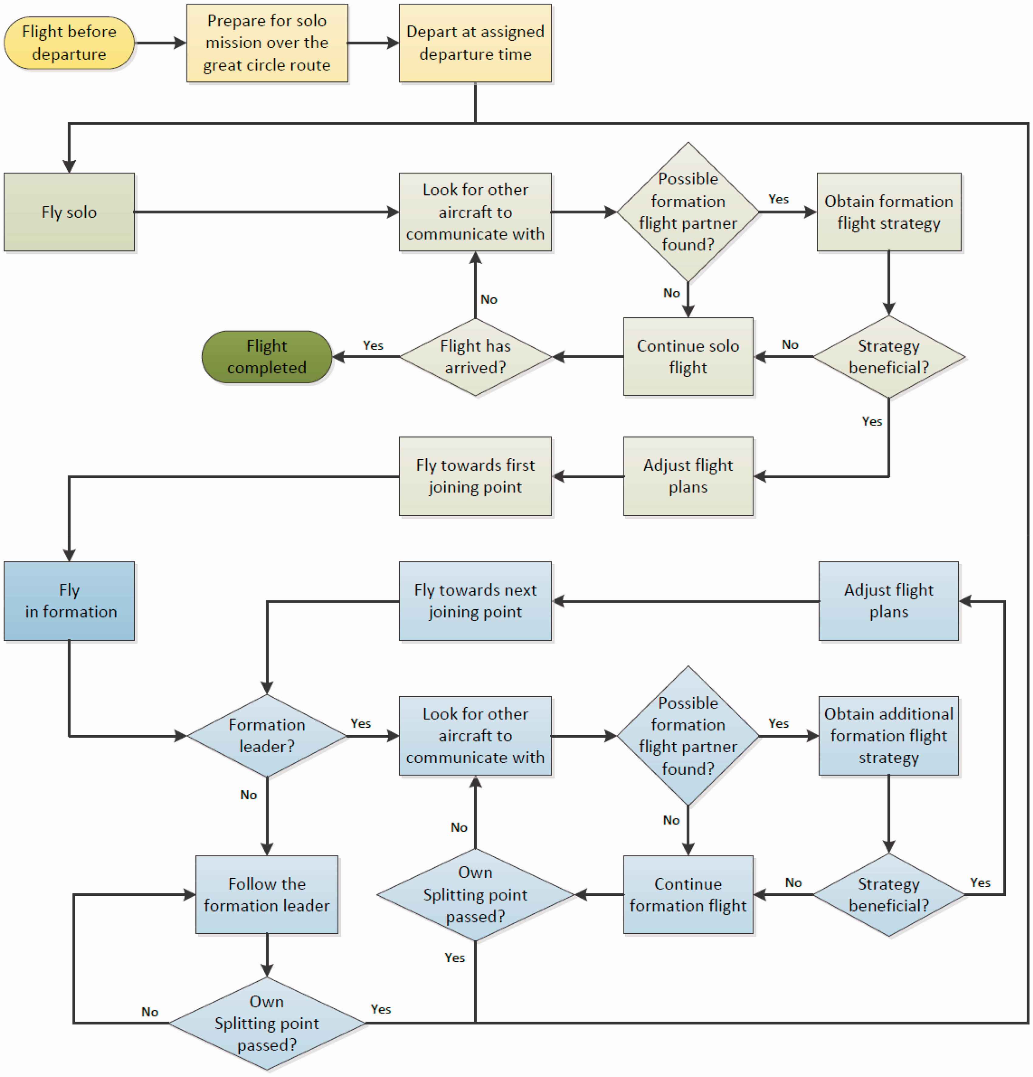

As soon as flights are ready, meaning that their take-off weight and great circle route form origin to destination have been determined, they depart at their assigned departure times. Note how each flight originally starts out as a solo flight that might possibly extend all the way up to the intended destination. This is a key feature of the developed decentralized approach; individual flights do not anticipate the use of formation flight. At some point in time, two neighboring flights may start communicating and commit to a formation flight. They alter their heading and speed in order to meet each other at the agreed time and location, the latter of which is called the “joining point”. The process during which aircraft readjust their flight path and speed to rendezvous at the joining point is hereafter referred to as the “synchronization” process. Once the decision to join a formation has been made, the aircraft involved stop communicating with other potential partners until the actual rendezvous has taken place.

When two, or more, flights have successfully completed their rendezvous, one of the aircraft involved needs to be assigned as the formation leader. A flight that does not lead a formation is referred to as a “follower”. In the present set-up, where only aircraft of the same type are considered, the least heavy aircraft of the two is designated as the lead aircraft. This order is based on the study conducted in Hartjes et al., ¹¹ where it is shown that it is beneficial to assign the heavy aircraft as follower, since it can benefit relative more from an induced drag reduction factor. Apparently, this more than offsets the fact that a light leader generates weaker wake vortices, thereby producing less benefit to the (heavy) follower. It is noted that the study reported in Marks and Gollnick ¹² arrives at a somewhat different conclusion about the preferred order, by showing that a formation is more likely to produce a fuel-saving benefit if the weight of the leader is higher than that of the follower. In Marks and Gollnick, ¹² the aerodynamic interactions within the formation are based on an aerodynamic model that differs from that employed in Hartjes et al., ¹¹ which essentially implements the model developed in Xue and Hornby. ⁶

A formation leader may, similarly to a solo flight, attempt to communicate with other aircraft so as to find additional partners to extend the formation flight string. In Figure 1 it can be observed that a formation leader follows the same decision scheme as when flying solo, but now on behalf of the entire formation. The formation leaders ensure that they only commit to subsequent formation joining options if it results in cumulative benefits. A formation continues to exist up until the “splitting point”, defined as the point where a flight leaves its formation. After passing a splitting point, a formation is split up into smaller formations or possibly individual flights that head off to their respective next splitting point or final destination.

Figure 1 suggests that each last segment of a mission is a solo flight segment. In both reality and within this study, this is most likely to occur and hence the process is represented as such. However, it is noted that the developed model allows flight strings with common destinations to locate their splitting point at this common destination.

Fuel consumption assessment

The transatlantic routes are modeled in this study as great circle paths from origins to destinations. Moreover, it is assumed that the entire route is flown in cruise at a constant altitude and at constant speed. The fuel consumption along the routes is estimated using the well-known Breguet-range equations, ¹³ assuming the absence of wind. The constant speed along the route is taken as the best specific-range speed at maximum take-off weight. This typically results in a speed close to the maximum cruise speed. Since we consider all aircraft to be of the same type, it also implies that all aircraft essentially fly at the same speed (except during synchronization flight legs) in this study. The parameters of the aircraft model employed in this study relate to a Boeing B777, and have been extracted from Kent and Richards ⁷ and Kent. ⁸

The actual take-off weight for a specific flight is calculated using the Breguet-range equation assuming that at destination the weight of the aircraft is equal to the zero-fuel weight plus the weight of the reserve fuel. Given the aircraft weight at destination, and the distance covered along the route, the aircraft weight at the origin can be assessed using the Breguet-range equation, for the assumed speed and altitude. To allow for the fact that aircraft may have to fly detours and thus longer routes in order to engage in flight formation, the initial fuel load is increased by 10%; the take-off weight of the aircraft is increased accordingly.

As indicated, in the present scenario aircraft essentially fly at one and the same speed throughout their flight. The only exception is when aircraft execute a synchronization flight leg in order to rendezvous with their formation partners, in which case one of the two aircraft has to slow down. Note that the minimum speed in a synchronization flight leg is the maximum endurance speed, which is the speed at which the lowest fuel consumption per unit of time is attained. ¹³ In case that flying at the maximum endurance speed is not sufficient to absorb the required delay time, the location of the joining point will need to be adapted. Flying a synchronization flight leg at a lower speed than the maximum endurance speed is not an option, as it will result in a fuel penalty.

In this study it is assumed that flying in a formation will generate a 10% reduction in fuel flow for any trailing aircraft in a flight formation. It is noted that several aerodynamic studies related to formation flight point out that the formation induced drag reduction increases as the number of aircraft in the formation string increases. ⁶ However, in this study this particular effect is ignored and each trailing aircraft in a formation essentially enjoys the same induced drag discount factor, regardless of the size of the formation string. Note that organizing the traffic flow into larger formation flights can still be very rewarding in the sense that the number of formation flight leaders that are needed (and that do not enjoy any drag reduction benefit) can be reduced in this way.

Formation flight routing

To generate routes for the assembly of formation flights, a routing method was used based on the study of Kent and Richards ⁷ and Kent. ⁸ In this approach, a formation flight route for two aircraft is obtained through the minimization of weighted distance. The routing method from Kent and Richards is extended herein to permit application within the developed decentralized approach.

Geometric routing method by Kent and Richards

In Kent and Richards ⁷ and Kent, ⁸ a simple geometric method to construct a formation flight routing is presented based on a classical mathematical problem posed by Fermat in the 17th century. The problem, illustrated in Figure 2, is posed as follows: given a triangle ABC (Figure 2(a)), find a point P such the that the sum of the distances $\left|\right|\mathit{AP}\left|\right|$ , $\left|\right|\mathit{BP}\left|\right|$ , and $\left|\right|\mathit{CP}\left|\right|$ is minimized. The geometric approach to construct the solution to this problem is illustrated in Figure 2(b).

Figure 2.

Geometric construction to locate the optimal joining point P (reproduced by permission of Dr Thomas Kent ⁸ ): (a) Triangle ABC with possible joining point P; (b) Circumscribed circles and subtending lines concurrent at an optimal point P.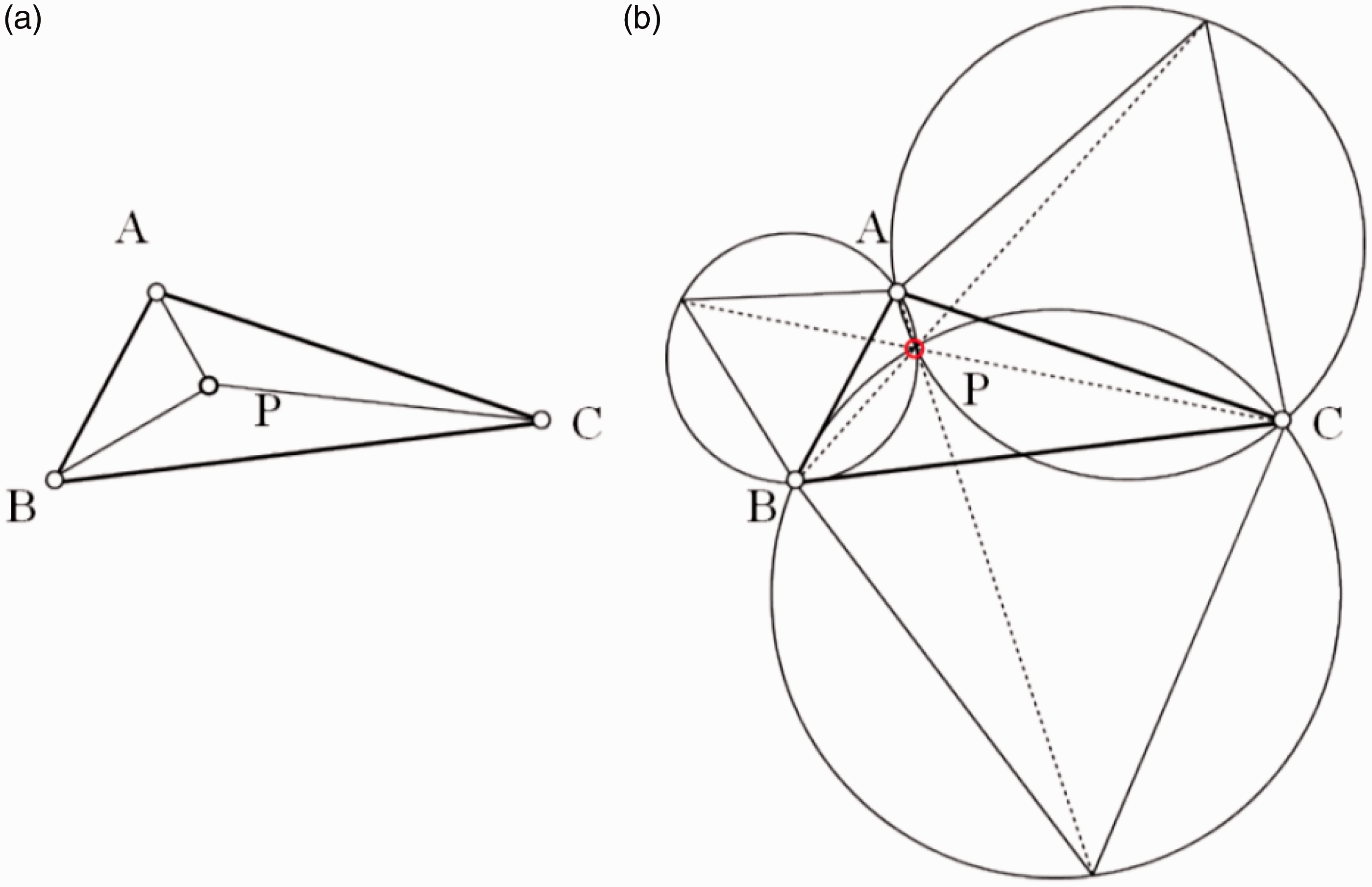

The method shown in Figure 2(b) is based on constructing outwardly three equilateral triangles along the sides AB, BC, and CA. Then the lines from the outer vertex of each new triangle to its opposite vertex of the original will intersect at a single point, which is the desired point P. Equivalently, point P can be found as the intersection point of the circumscribed circles of each of the three new equilateral triangles.

Fermat’s problem provides a good analogy to the formation flight assembly problem, if it is assumed that fuel consumption is proportional to the distance covered. However, it is readily clear that the fuel consumption per unit distance along the solo arcs $\left|\right|\mathit{AP}\left|\right|$ and $\left|\right|\mathit{BP}\left|\right|$ differs from that on the formation flight arc $\left|\right|\mathit{PC}\left|\right|$ . To resolve this issue, Kent and Richards formulated a weighted-arc version of the problem, where the arc weights reflect the different fuel consumption per unit distance. More specifically, to represent the cost of flying a unit of distance, the arc weights w_A, w_B, and w_C are introduced for the segments AP, BP, and PC, respectively. Note that the value of w_C is typically set equal to the combined values of w_A and w_B, while applying some discount factor to represent the fuel savings due to induced drag reduction of the trailing aircraft.

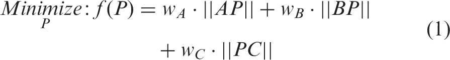
Thus, in the modified problem the location of the joining point P has to be selected such that the total cost of distance, expressed by the following equation is minimized

$$\begin{array}{c}{\mathit{Minimize}:}_{P}f(P)=w_A·\left|\right|\mathit{AP}\left|\right|+w_B·\left|\right|\mathit{BP}\left|\right|\\ +w_C·\left|\right|\mathit{PC}\left|\right|\end{array}$$

(1)

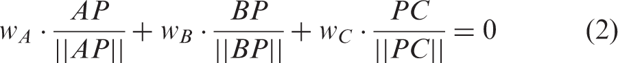
Following Kent and Richards, the location of point P that minimizes equation (1) must satisfy the vectorial equilibrium condition expressed by the following equation

$$w_A·\frac{\mathit{AP}}{\left|\right|\mathit{AP}\left|\right|}+w_B·\frac{\mathit{BP}}{\left|\right|\mathit{BP}\left|\right|}+w_C·\frac{\mathit{PC}}{\left|\right|\mathit{PC}\left|\right|}=0$$

(2)

Application of the law of cosines to equation (2) yields expressions for the intersection angles ∠APB, ∠APC, and ∠BPC. Since angle ∠APB represents the intersection angle between the two solo legs AP and BP, it is referred to as the “formation angle”. Equation (3) gives the expression for the resulting formation angle θ_f

$${\theta }_f={\text{cos}}^{-1}(\frac{-w_A^2-w_B^2+w_C^2}{2w_A{w}_B})$$

(3)

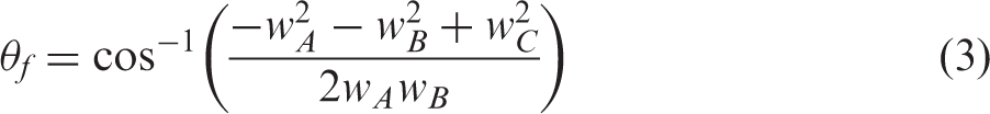
Note that the formation angle θ_f only depends on the routing weights w_A, w_B, and w_C. The formation angle is illustrated in Figure 3. It is noted that as long as the weights w_A, w_B, and w_C are not altered, also the formation angle θ_f remains unaffected. As a result, point C can be shifted freely along line PC, without altering the solution.

Figure 3.

Illustration of the formation angle.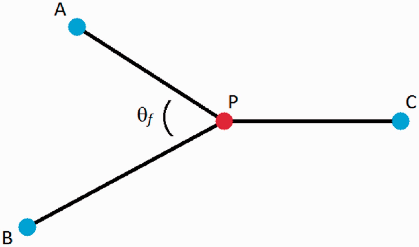

The method for locating point P can be extended to a scenario in which the two flights do not have a common destination C. Figure 4 illustrates two solo routes connecting origins A and B to destinations C and D, respectively. The joining point J and the splitting point S are to be determined. Since the formation angle condition must be satisfied at both J and S in order to minimize the weighted distance, one can draw two circular arcs from A to B and from C to D along which the formation angle is constant and equal to the value obtained from equation (3). These arcs are displayed in Figure 5.

Figure 4.

Illustration of example solo routes AC and BD.

Figure 5.

Geometric construction of the formation flight route.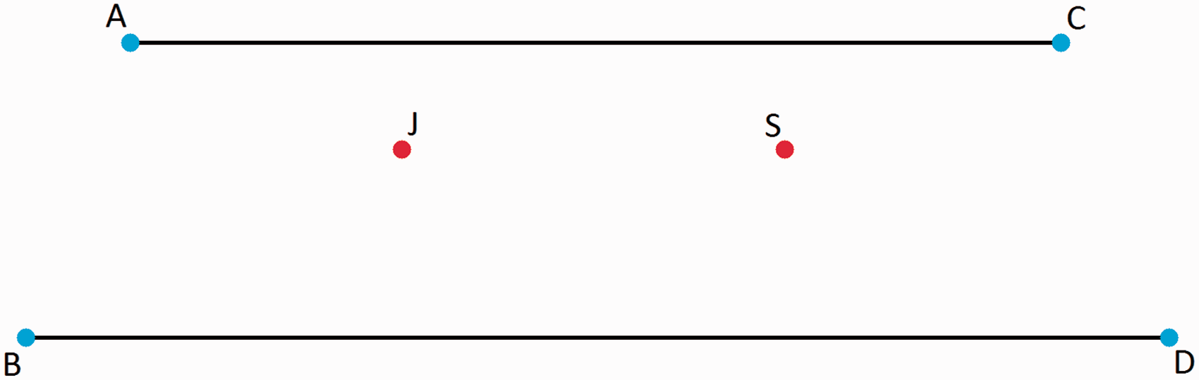

Point X₁ in Figure 5 is obtained by making use of the fact that equation (4) holds in triangle ABX₁

$$\left|\mathit{AB}\right|:\left|{\mathit{BX}}_1\right|:\left|X_{1}A\right|=w_C:w_A:w_B$$

(4)

Mirroring the described steps at destinations C and D provides point Y₂. The locations of J and S that minimize the weighted distance from A to C and from B to D are obtained from the intersections of the line from X₁ to Y₂ and the arcs of constant formation angle.

Figure 6 illustrates how a formation flight route would change when w_A > w_B. The (dashed) green route shows the effect on the formation flight route of using w_A > w_B with respect to the (solid) blue route, where w_A = w_B. Since the flight from A to C is now considered more expensive per unit of distance, the detour for the corresponding aircraft is reduced in length.

Figure 6.

Flight formation route assembly; for the blue (solid) route: w_A = w_B; for the green (dashed) route: w_A > w_B.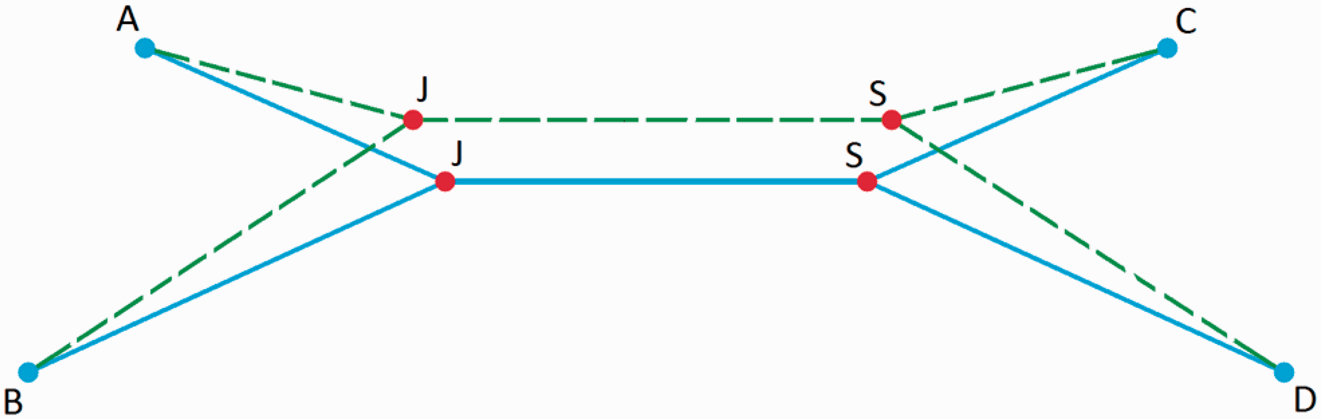

Accommodating synchronization in the basic routing method

In contrast to the work of Kent et al., or to any centralized approach, the decentralized approach that is developed herein considers formation flight to be an in-flight option. Therefore, any set of flights that will use the formation routing method to identify potential savings, will do so while flying towards their respective destinations. For formation flight to be realized, the route must be constructed such that the two (strings of) aircraft are able to arrive at the joining point simultaneously. Ensuring the latter is here referred to as enabling “synchronization”. For relatively symmetric solo segments connecting at the joining point, synchronization may often be accomplished by slightly slowing down one of the aircraft. However, if the original formation flight route does not permit synchronization in this way, the joining point must be relocated to enable a stretch of the connecting flight legs. Accordingly, one aircraft is slowed down to V_min (i.e. the maximum endurance speed) while the other maintains its cruise speed V_cruise (which is close to the maximum cruise speed). It was chosen to restrict the possible relocations of the joining point J_new to be on the original formation flight segment J_oldS. Moving J closer towards S will postpone the initiation of formation flight, but will also reduce the detours that both aircraft have to fly.

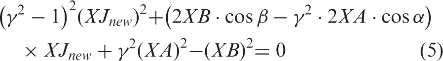
In Figure 7, the current locations A and B, along with the originally determined joining point, labelled J_old, are shown. Point X shown in Figure 7 is defined as the intersection of the segments AB and X₁J_old. Application of the law of cosines to the triangles AXJ_new and BXJ_new, yields the following quadratic relation, for any given speed ratio γ = V_B/V_A

$$\begin{array}{c}({\gamma }^2-1{)}^2({\mathit{XJ}}_{\mathit{new}}{)}^2+(2\mathit{XB}·\text{cos}\beta -{\gamma }^2·2\mathit{XA}·\text{cos}\alpha )\\ \times {\mathit{XJ}}_{\mathit{new}}+{\gamma }^2(\mathit{XA}{)}^2-(\mathit{XB}{)}^2=0\end{array}$$

(5)

where it is assumed that speed V_A is equal to V_min and speed V_B equal to V_cruise in the sketched geometry in Figure 7 (AJ_new < BJ_new). Equation (5) can be solved for the side length XJ_new that can subsequently be used to construct the location of the new joining point J_new that enables synchronization. However, it is conceivable that equation (5) still does not yield a feasible root. In this case, excess delay time needs to be absorbed by holding one of the aircraft at the joining point. However, when the latter situation does occur, usually the formation option turns out to be less favorable then flying solo.

Figure 7.

Relocation of joining point J to enable synchronization.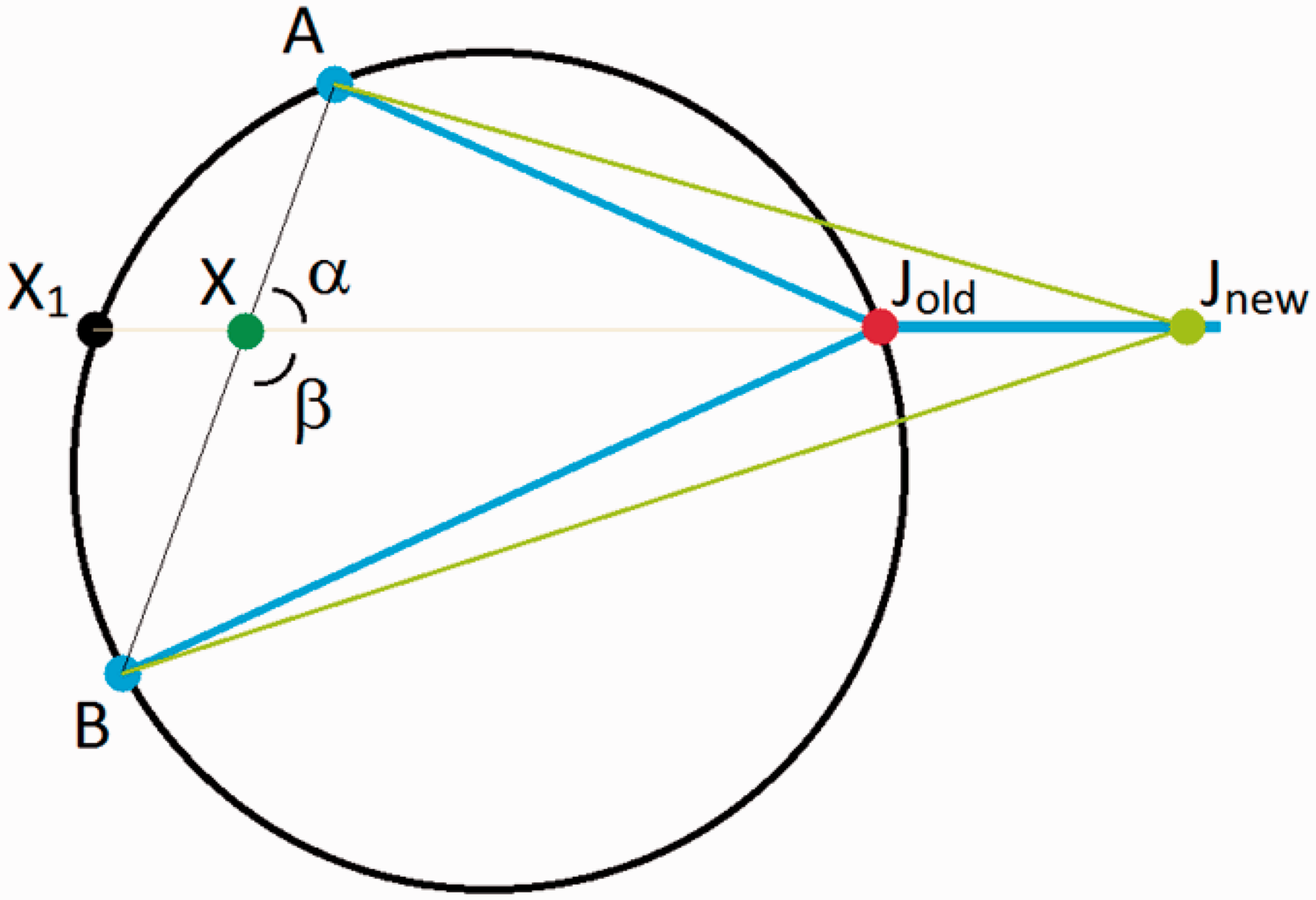

The geometric approach presented herein is inherently planar in nature; however, it can be extended to hold for problems on a sphere.^7,8 This latter option has not been pursued in this study; rather the great circle routes connecting the various O/D pairs were projected on a plane by means of the so-called azimuthal equidistant projection method, ¹⁴ so that the original planar geometric approach can be retained. The azimuthal equidistant projection method has the property that all distances from the center are rendered correctly to scale and that all points on the map are at the correct azimuth (direction) from the center point. Here, the center point is defined by the mean longitude and mean latitude of the considered origin and destination airports. By using this particular projection method, the relative locations of the origins and destinations, as well as the route lengths and relative flight headings remain reasonably well preserved in the transformation. Since these route characteristics are most relevant for the success of the formation flight implementation, the selected projection method is considered appropriate for this study.

Example of formation flight routing

In this subsection, a simple example is presented to demonstrate the overall formation flight synthesis process. Figure 8 shows four randomly selected great circle routes connecting the origin airports on the left side of the graph with the destination airports on the right side of the graph. Figure 9 displays the corresponding formation flight routes that were synthesized for the same O/D pairs based on the proposed operational concept.

Figure 8.

Solo routes in the formation flight routing example.

Figure 9.

Assembly of formations in the formation flight routing example.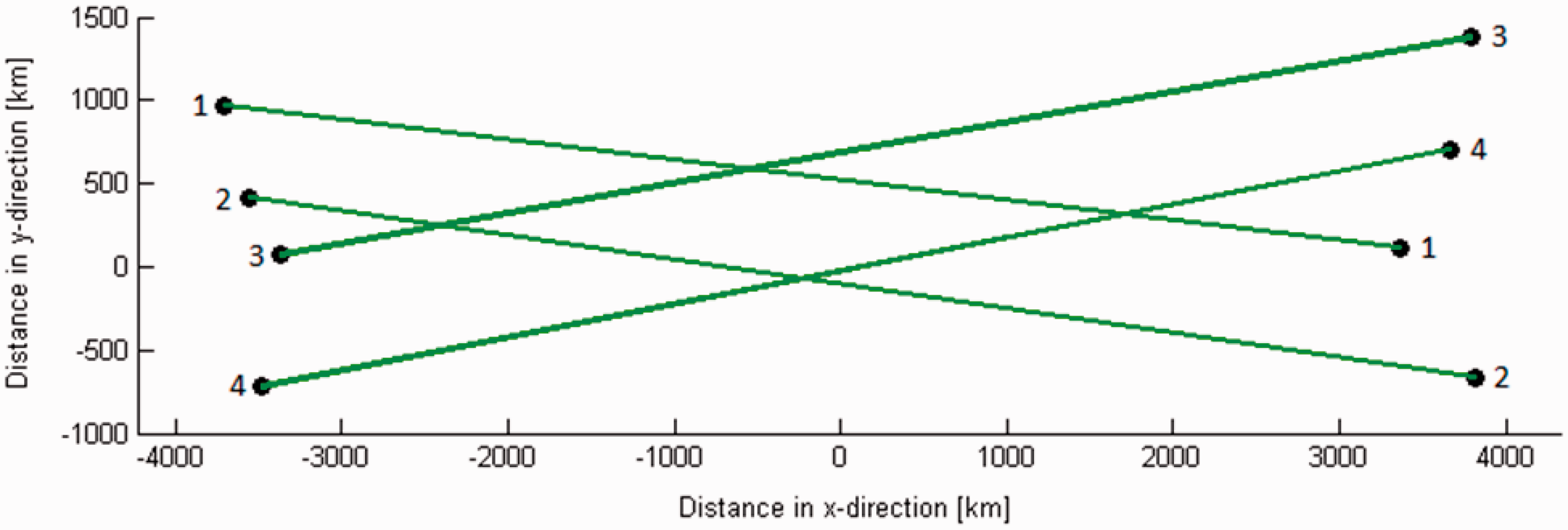

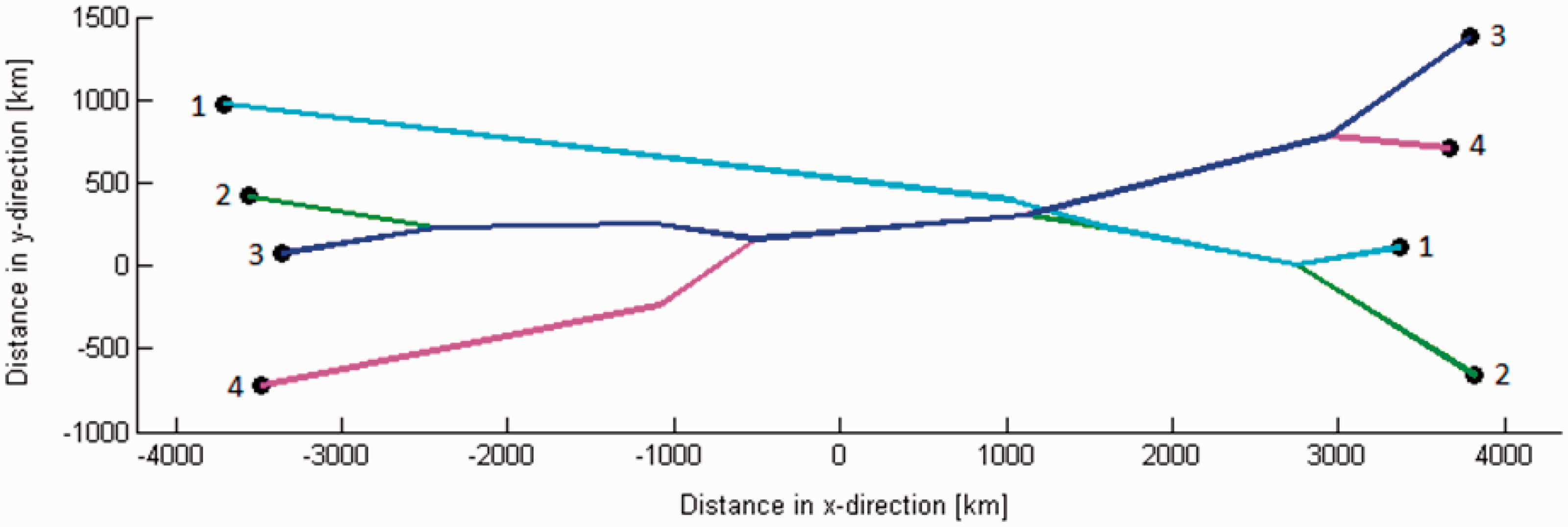
A close inspection of Figure 9 reveals that Flights 2 and 3 commit to a formation flight immediately after departure. However, Flight 1 does not encounter a potential formation flight partner in the initial stage of its mission, and also Flight 4 is out of communication range of any partner during the first part of its mission. When the flights reach a down range position at about 1000 km, Flight 4 and the two-ship formation (involving Flights 2 and 3) enter each other’s communication circles. A formation option is then assessed and subsequently accepted, resulting in the assembly of a three-ship formation. As the three-ship formation reaches the down-range position 0 km, no profitable formation joining options have been encountered that would include Flight 1. After passing the 1000 km down range mark, Flight 2 leaves the three-ship formation and becomes available again for communication, and indeed commits to a new formation flight, teaming up with Flight 1. The two resulting two-ship formations fly on towards their splitting points, after which all flights conclude with a solo segment. The example clearly demonstrates the flexibility of the proposed concept, showing that a flight (in this case Flight 2) can be part of more than one formation.

Transatlantic case study

Baseline scenario

The proposed operational concept, as presented in Figure 1, is applied in a case study involving 347 eastbound transatlantic flights. The routes included in the case study, shown in Figure 10, are obtained from an available real-life data set ¹⁵ by means of selecting the longitude/latitude coordinates of all origins and destinations. In the scenario considered, it is assumed that each flight can potentially join in formation with any other flight in the network (regardless of airline or alliance membership).

Figure 10.

Route set used in the case study (created using Great Circle Mapper at www.gcmap.com).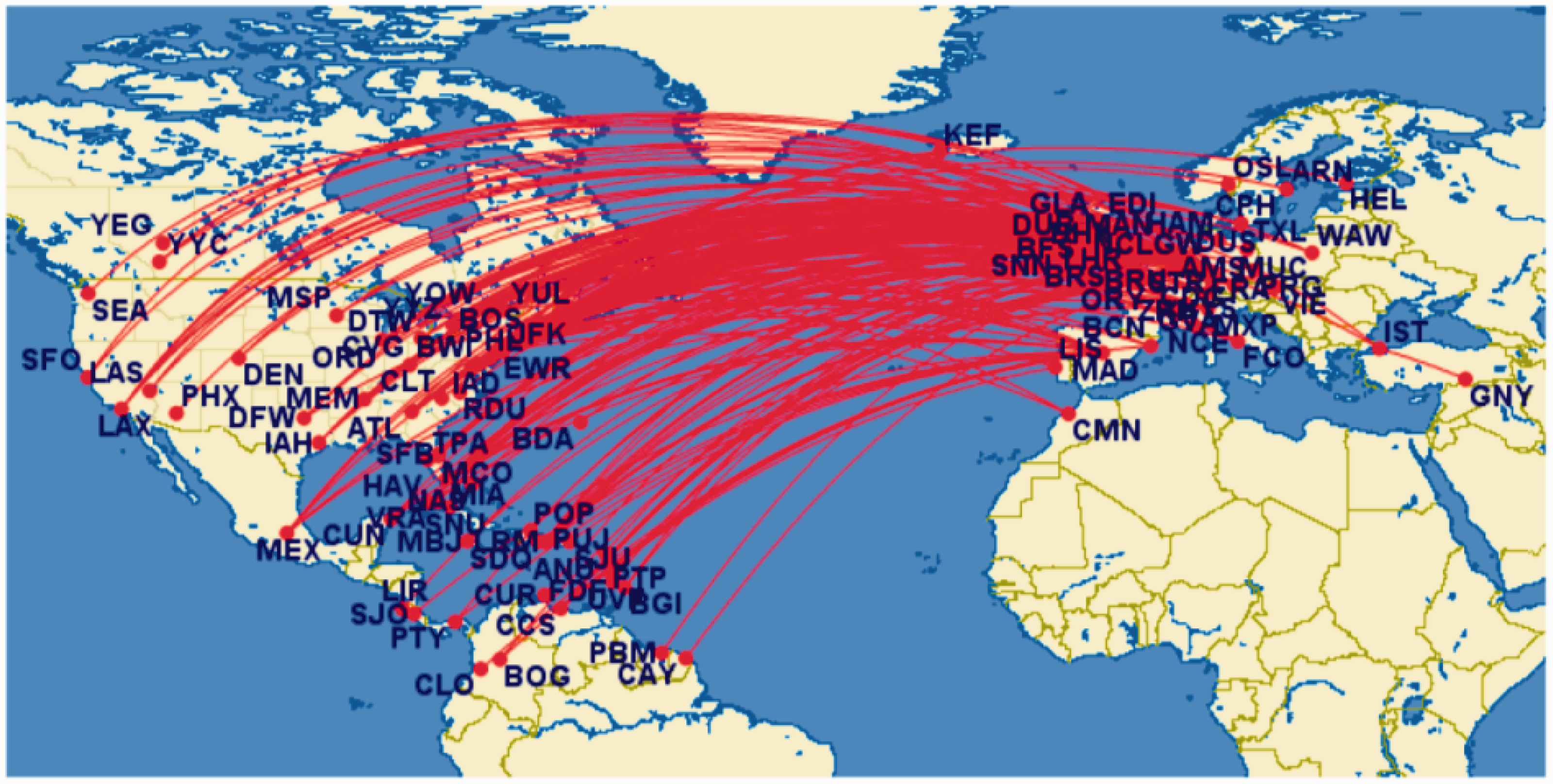

In the simulation set-up, the location of each aircraft along a great circle route is updated with a time step of 5 min. This time step size (dt) was found to be sufficiently small to demonstrate the potential of the developed method. All other aircraft parameters, such as speed, heading, current weight, fuel flow settings, and formation flight status are only revisited at a position update when required. There are three types of events that may trigger such an extended update: (i) two flights commit to a formation flight option, (ii) a joining point is passed, or (iii) a splitting point is passed.

In the baseline scenario a fixed communication range of 250 km has been assumed and all aircraft successfully depart according to the original (unperturbed) schedule. Any formation flight option that saves any amount of fuel is immediately accepted, regardless of the increase in trip time that flights will experience. In the baseline model configuration, a typical simulation of the baseline scenario requires about 6 min of calculation time on a standard PC, including result visualization in graphs and the creation of an animation.

Figure 11 shows several snapshots of the simulation results at various instances in the flight. The three subfigures of Figure 11 display a snapshot of the situation (using azimuthal equidistant projection) at, respectively, 200, 400, and 600 min into the flight. The colored dots shown in the subfigures of Figure 11 mark either the position of a flight at the considered time instance or the location of an origin or destination airport (blue dots). The position of a flight that is “engaged” to a formation is displayed as a cyan dot. A flight is referred to as “engaged”, when it has committed to join a particular flight formation, but is still flying towards the rendezvous point.

Figure 11.

Snapshots of flight formations in the baseline scenario (azimuthal equidistant projection).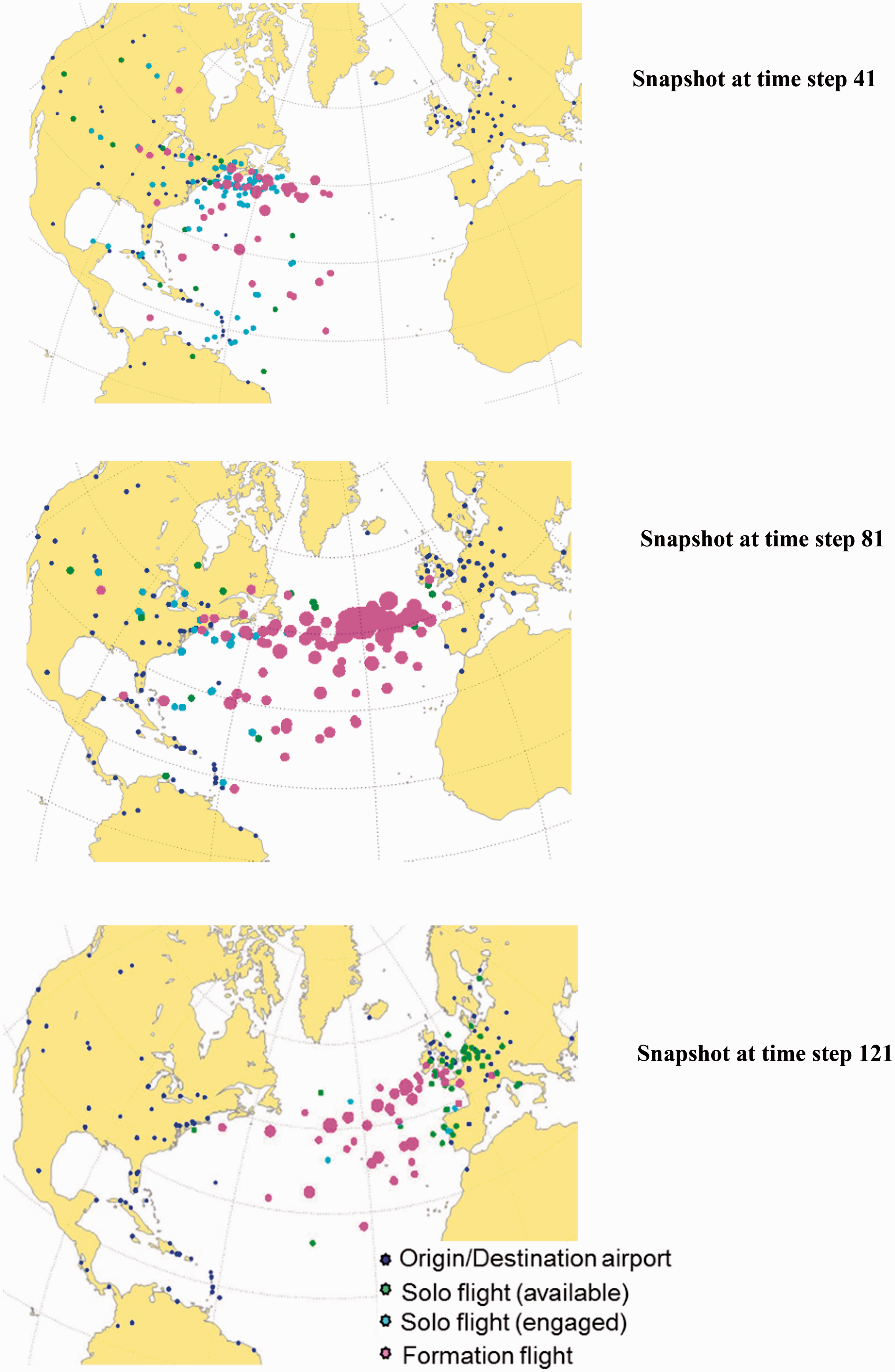

From the origins (blue dots) shown on the left side in the subfigures of Figure 11, flights are departing. As flights proceed towards their destination, they start out as green dots, indicating that they are still flying solo. After some time, most flights engage to another flight to join in formation, causing them to change their course; these engaged flights are displayed as cyan dots in Figure 11. Some flights continue flying solo, even though they have been in the air for some time. Note that most of these solo flights are not in the vicinity of other aircraft that are allowed to communicate. The purple dots show the assembled formations; the size of the purple dot is proportional to their size. At only 200 min into flight, already two formations of size 5 have been assembled. In the upper region of the top subfigure in Figure 11, many cyan-colored flights can be seen that are flying along synchronization segments towards their designated joining points.

In the middle subfigure of Figure 11, the traffic situation is shown at 400 min into the flight. It can be seen that at this stage the supply to the eastbound stream of aircraft has started to dry up. As a matter of fact, all flights have departed from their origin airports at this stage of the simulation. Many formations of different sizes have emerged in the upper part of the figure. The largest formation in use at this point, or at any point, comprises 15 aircraft. A closer inspection revealed that this particular formation was assembled when a formation string of size 8 and a formation string of size 7 accepted a late option to join in formation. The green dots at the right side of the graph indicate flights that have split off from their formations; they are heading towards their destination by means of a solo flight segment.

The bottom subfigure of Figure 11 shows the traffic situation another 200 min later, at which point an appreciable number of flights have already reached their destination. Many solo flights are completing their final segment towards their destination. While only three cyan dots can be discerned at this particular instance, it was found that several flights that at an earlier stage split off from a formation, re-engage to a new formation in the final stage of their respective missions. It is not surprising that a few of the flights that were last in line to depart, do not manage to join a formation. The combination of the location of their origin and their departure time prevents them from encountering any formation flight partner.

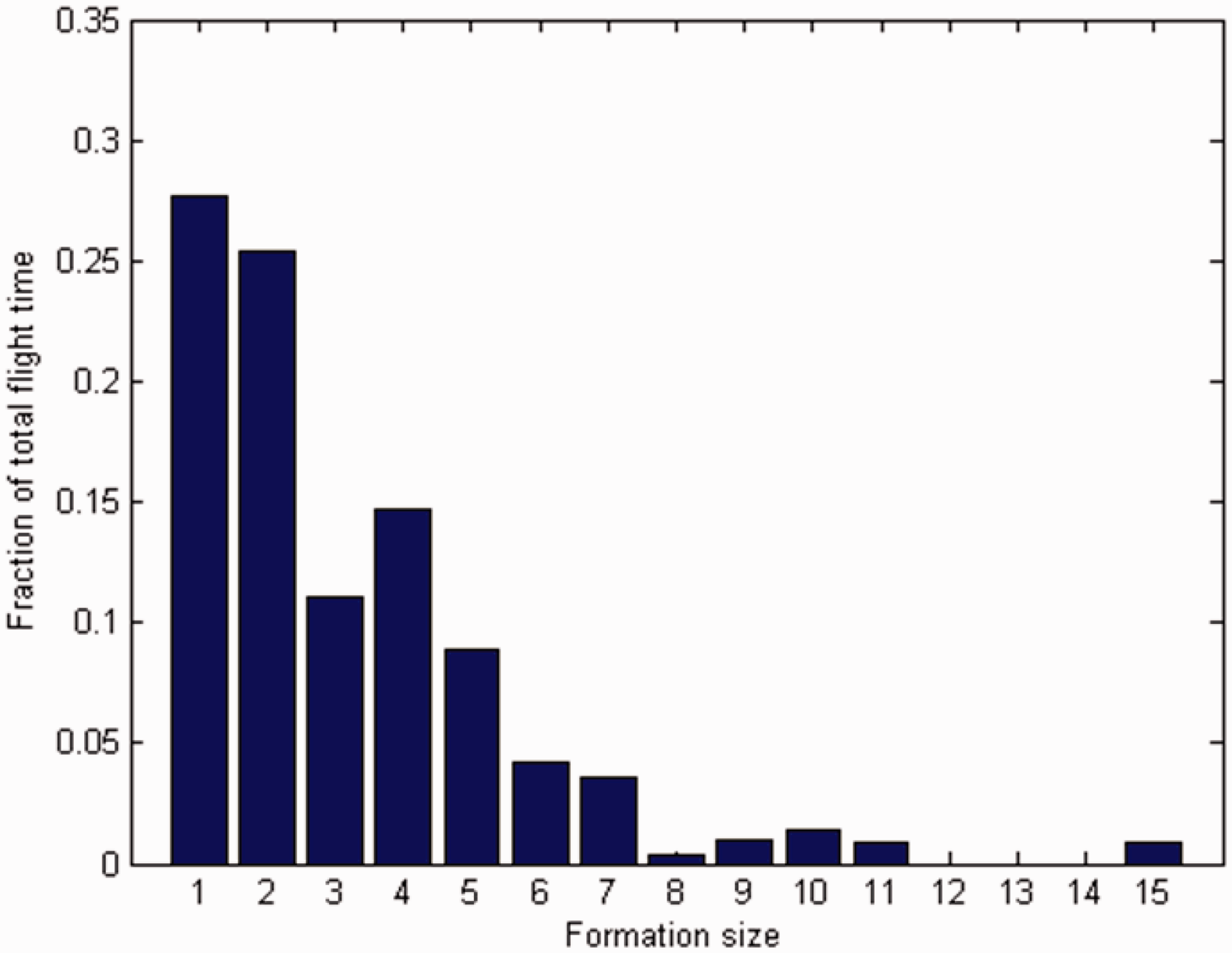
Figure 12 presents the additional flight times that aircraft have to incur due to the implementation of formation flight. The average additional flight time is about 17.6 min. Figure 13 shows the fraction of total flight time distribution over the used formation sizes. This fraction is calculated by dividing time spent in a formation of given size aggregated over all flights by the total flight time aggregated over all flights. It is noted that 72% of the total flight time is spent in a formation. Significant use is made of formations that comprise up to seven aircraft. Occasionally, larger formations occur.

Figure 12.

Additional flight time distribution in the baseline scenario.

Figure 13.

Flight time distribution over formation sizes in the baseline scenario.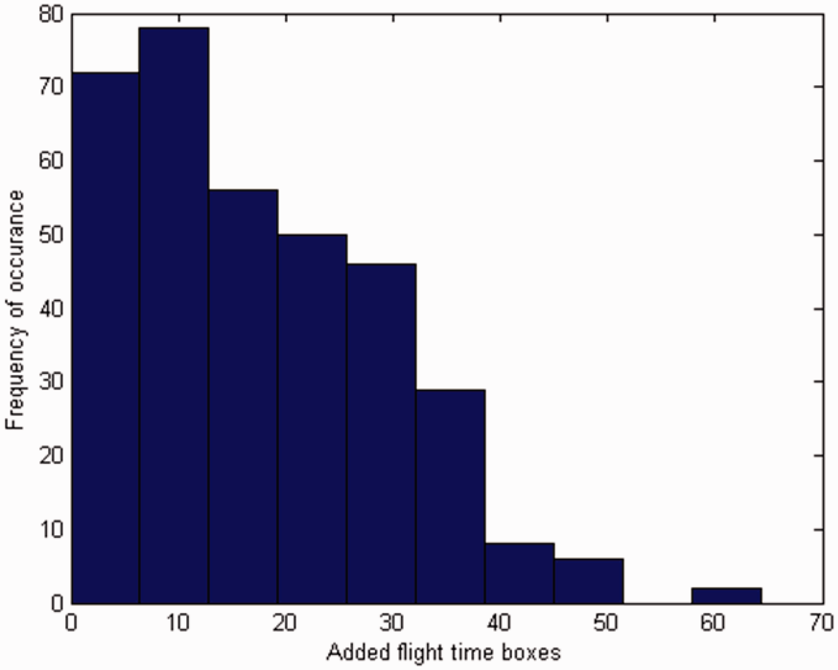

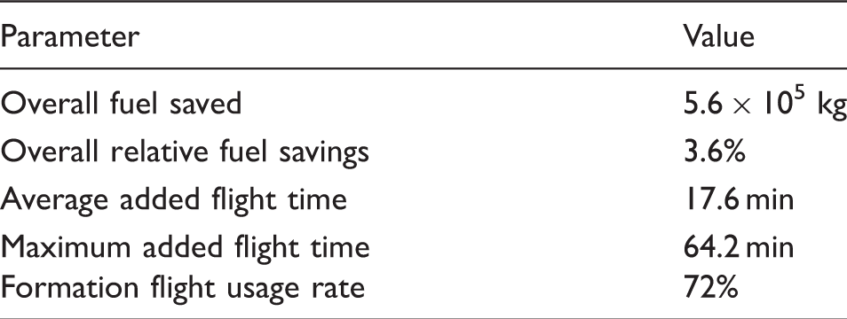
Table 1 summarizes the main performance results obtained in the conducted simulation. The overall obtained fuel savings amount to 3.6% relative to using only solo flights. For operations with the standard aircraft that was defined (B777), this would be equivalent to saving 5.6 × ċ10⁵ kg of fuel across the network. An in-depth analysis of the used flight trajectories revealed that significant fuel investments are required to achieve synchronization. This obviously restricts the overall fuel-saving potential to quite an extent.

Table 1.

Summary of results of the baseline scenario.

Parameter	Value
Overall fuel saved	5.6 × 105 kg
Overall relative fuel savings	3.6%
Average added flight time	17.6 min
Maximum added flight time Formation flight usage rate	64.2 min 72%

A similar simulation study was conducted for a scenario in which flights were randomly delayed. The attained overall fuel savings and the use of formation flight were found to be very similar to the baseline case. The decentralized implementation of formation flight allows delayed flights to participate in formation flight with any aircraft that it may still encounter.

Adding an incremental flight time constraint to the baseline scenario

The significant additional flight times that were found in the baseline scenario, as shown in Figure 12, motivated a revised model set-up in which the additional flight time was inherently limited. A limit was introduced on the additional flight time that an aircraft was allowed to incur from a single flight formation decision. In this study, a 10-min limit is applied to each formation joining decision in the simulation. Since it is possible that an aircraft is involved in multiple sequential formation joining decisions (let’s say, L decisions), the overall delay for a flight can accumulate to a maximum of L × 10 min.

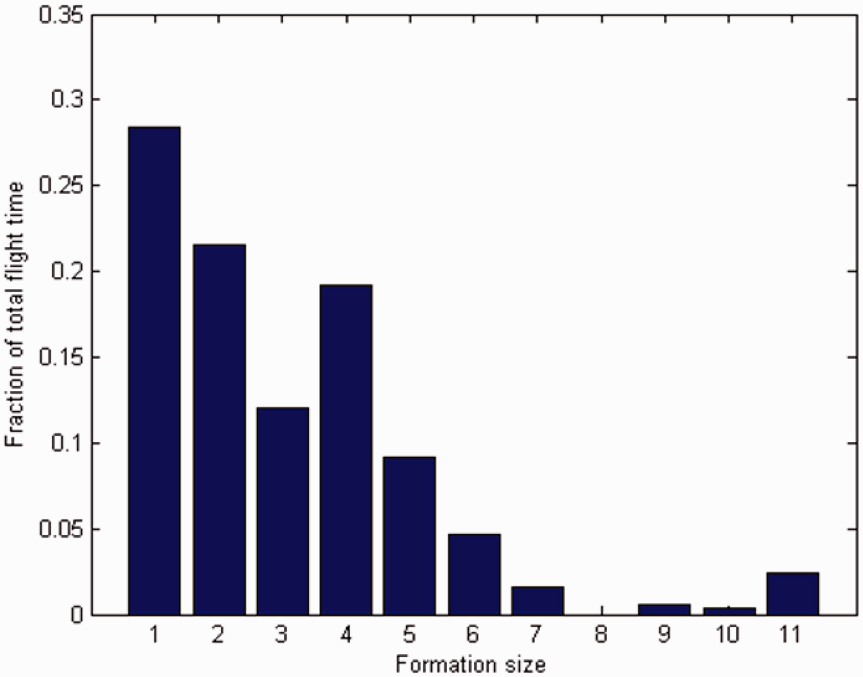
Figure 14 presents the new distribution of additional flight times over all the involved aircraft. The average additional flight time has decreased to about 9.9 min. Figure 15 displays the new distribution of the fraction of total flight time over the used formation sizes. While the usage rate of formations of size 4 has increased, the general use of formations is quite similar, albeit that the largest formation string size is somewhat smaller. Remarkable is the fact that the overall obtained fuel savings have actually increased relative to the baseline case to 4.2%. This striking result can be explained from the fact that a greedy algorithm has been employed, as will be outlined in more detail in the next section.

Figure 14.

Additional flight time distribution in the modified scenario.

Figure 15.

Flight time distribution over formation sizes in the modified scenario.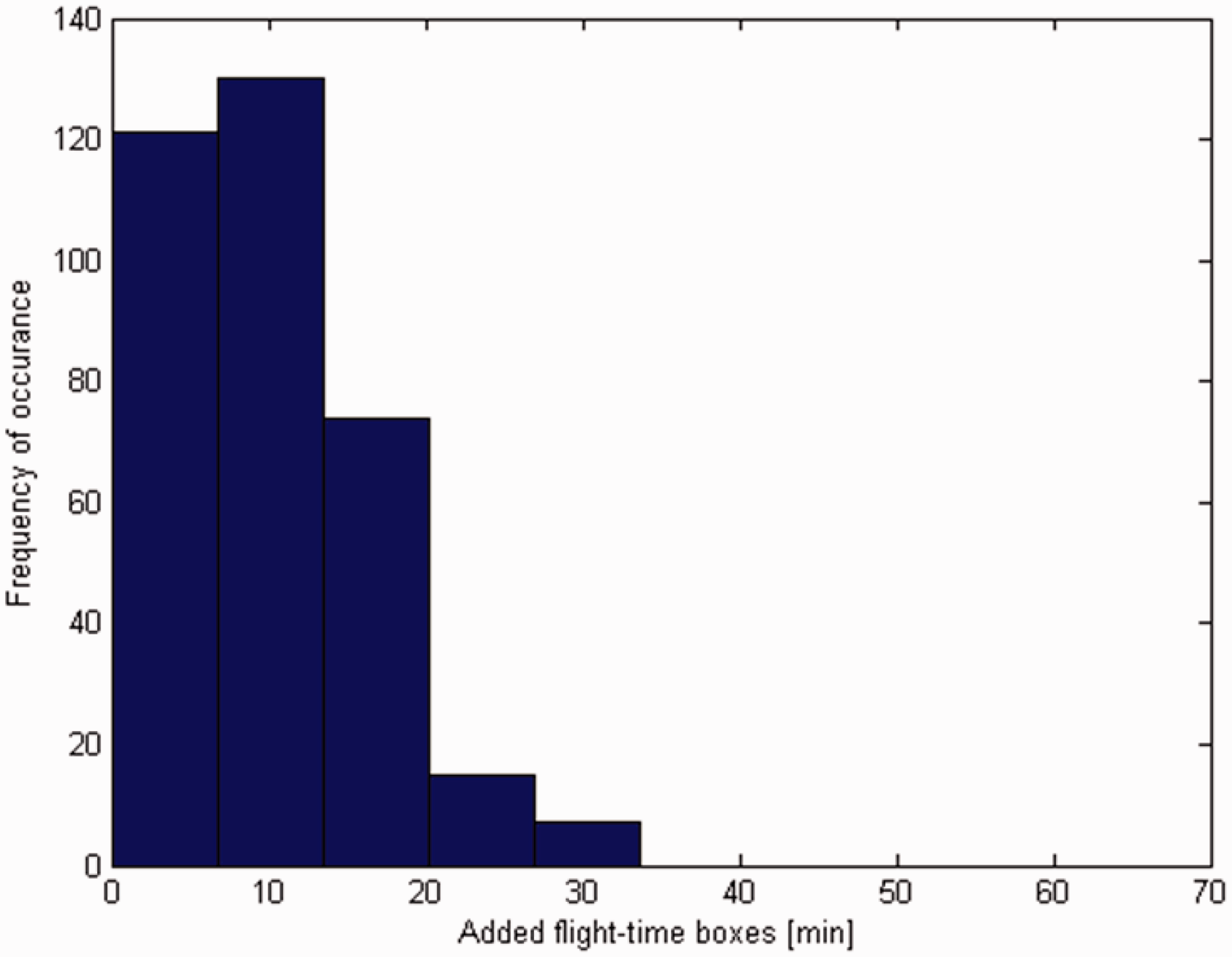

Influence of communication range

Since the communication range directly determines the nature of the formation flight options that flights can encounter, a study has been performed that assesses how the overall obtainable fuel savings vary with the communication range. Given the positive relation that was observed between the overall achieved fuel savings and the limit on additional flight time, the communication range is varied with and without imposing this limit.

Figure 16 shows the results of 120 (60 per scenario) Monte Carlo simulations of the 347 transatlantic flights in this case study, featuring stochastic variations in schedule delay. Similar to Xue and Hornby, ⁶ the randomly generated departure times are sampled from a normal distribution with a mean of 0 min and a standard deviation of 15 min. The solid (blue) line in Figure 16 represents the results for the scenario without the limit on additional flight time. As the communication range is increased, flights are allowed to communicate with other flights that are further away. Up to a communication range of 50 km, a steep increase in attainable overall fuel savings is recorded. This can be explained by the fact that the number of encounters between aircraft has increased significantly. This leads to more formation flight options being evaluated and, evidentially, accepted. For communication ranges of 50 to 120 km, the increase in obtained fuel savings persists, albeit with a smaller average gradient. Indeed, the system model still finds additional/more beneficial formation flight options at these conditions. At a communication range of about 120 km, the maximum attainable fuel savings are recorded. These savings amount to about 4.2% relative to solo flights, averaged over all simulated routes. The standard deviation in the savings remains remarkably small. Increasing the communication range from 120 to 600 km reveals a gradual decrease in the achieved fuel savings, which appear to plateau at around 3.0%. This gradual decrease in obtained savings can be readily explained. When the communication range is increased beyond 120 km, formation flight options that require relatively larger detours are encountered. Some of these will be accepted by the greedy communication algorithm, as long as they result in (marginal) cumulative fuel savings. Apparently, these marginally beneficial, “premature” formation options affect the global fuel-saving potential, as the overall obtained fuel savings decrease when the communication range is increased beyond 120 km.

Figure 16.

Obtainable fuel savings vs. communication range; Solid (blue) line: no limit on additional flight time; Dashed (red) line: limited additional flight time.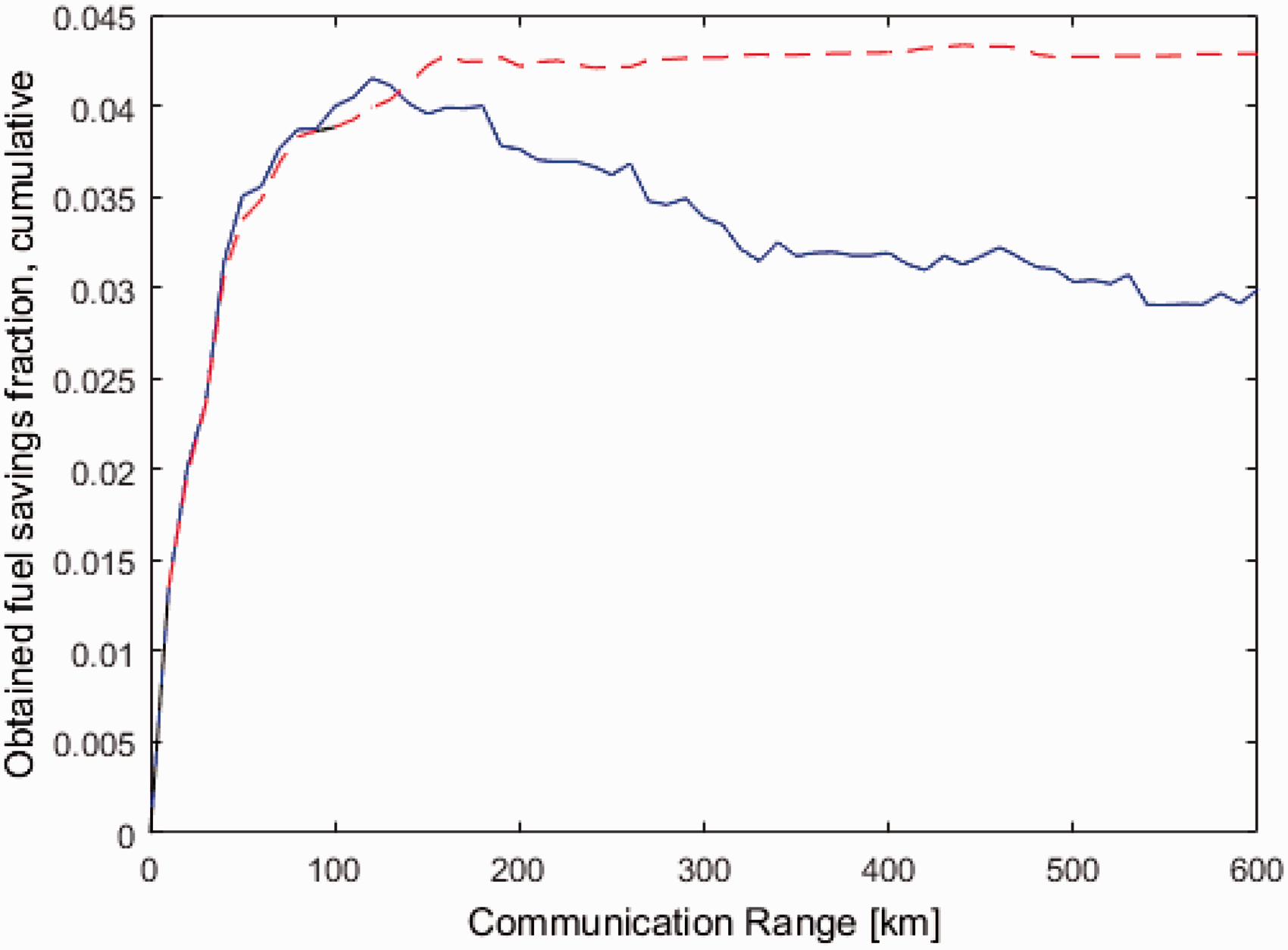

The dashed (red) curve in Figure 16 relates to the simulation results for the scenario where the limit on additional flight time is included. Note that in contrast to the original (unconstrained) solution, the overall fuel savings are maintained with increasing communication range. It is concluded that the imposition of a limit on additional flight time (per formation joining decision) counteracts the negative effect of a larger communication range on the overall attainable fuel savings, by precluding formation flight options that require large detours to establish formation flight. The largest estimated overall fuel saving, which amounts to 4.3%, is achieved at a communication range of 440 km, assuming a limit on additional flight time of 10 min per aircraft per formation joining option.

Conclusions

This study proposes a decentralized cooperative planning system for the efficient routing and scheduling of flight formations. In the transatlantic case study that was presented, the planning system proved to be flexible, reliable, and efficient. The formation flight routes that were generated exhibited many similarities to those found in the literature. However, in contrast to most approaches in the literature, the decentralized approach proposed herein allows the assembly of large formation strings, not limited in size.

Additionally, this work includes the use of consecutive formation flight options (enabling to gradually extend formation strings, as well as to re-join a formation), which yields a significant increase in the overall formation flight usage rate. Introducing formation flight as an in-flight option enables delayed flights to contribute to the fuel-saving objective.

It is noted that there are many important safety and regulatory issues, along with potential station keeping problems (especially in turbulent weather conditions) that need to be addressed before the implementation of (large) flight formations can take place at an operational level. However, in this study these challenges have not been addressed, but rather this study has been aimed at getting a better understanding of achievable fuel savings in (large) flight formations.

For future research it is recommended to explore improved agent-based strategies, including non-circular communication ranges and the possibility for aircraft to communicate with multiple neighbors concurrently. It is expected that especially the latter option will improve the quality of the flight formation decisions. Delayed flights do not pose challenges to the decentralized approach to the formation flight implementation. However, the developed decentralized approach may bring about significant fuel penalties to achieve synchronization. Possibly, these penalties can be attenuated by applying some form of pre-flight planning. These notions suggest a hybrid approach to the formation flight planning that incorporates both centralized and decentralized elements. This research direction will be explored in a follow-up study.